Resonant excitation amidst dephasing: An exact analytic solution

Abstract

An exact analytic solution is presented for coherent resonant excitation of a two-state quantum system driven by a time-dependent pulsed external field with a hyperbolic-secant shape in the presence of dephasing. Analytic results are derived for the amplitude and the phase shift of the damped Rabi oscillations.

I Introduction

Coherent resonant excitation represents an important notion in quantum mechanics Shore ; Allen-Eberly . Resonant pulses of specific pulse areas are widely used in a variety of fields in quantum physics, including nuclear magnetic resonance, coherent atomic excitation, quantum information, and others. Resonant excitation allows to establish a full control over the quantum system, particularly in a two-state system, and realize any unitary transformation (qubit rotation) in it. Particularly important transformations include complete population transfer (transition probability $P=1$), complete population return ($P=0$) and Hadamard transformation ($P=\frac{1}{2}$).

Crucial conditions for resonant coherent excitation are resonance (the frequency of the external field must be equal to the Bohr transition frequency) and coherence. Deviations from resonance (detuning) are detrimental and lead to rapid departure of the transition probability from the desired value. In this respect, an alternative to resonant excitation is provided by adiabatic excitation adiabatic , which is robust against such variations.

Even more crucial for resonant excitation is coherence. Incoherent excitation, as described by Einstein’s rate equations, allows only partial population transfer, e.g., at most 50% in a two-level system with equal degeneracies of the two levels Shore . Deviations from perfect coherence, which can be described by the quantum Liouville or Bloch equations, inevitably cause departure from the desired unitary transformation. Two general types of decoherence processes can be present: depopulation (e.g., due to spontaneous emission or ionisation) and dephasing (e.g., due to elastic collisions, field fluctuations, coupling to the environment, etc.).

In this paper, we present an exact analytic solution for pulsed resonant excitation of a two-state system in the presence of pure dephasing. Dephasing is recognised as one of the main obstacles in quantum information and the availability of precise analytic estimates of its effect can be very useful and important. We derive the exact solution of the Bloch equation for a hyperbolic-secant pulse shape and a constant dephasing rate. We provide examples of the general solution, which is expressed in terms of gamma functions, in various special cases of interest, e.g. for pulses with specific pulse areas. These results allow us to determine explicitly the deviations from the desired probabilities caused by the dephasing.

This paper is organised as follows. In Sec. II we describe the model and present the exact analytic solution, which is derived in the appendix. In Sec. III we analyse in some detail various special cases. In Sec. IV we give a summary of the results.

II Analytic model

II.1 The Bloch equation

Dephasing processes can be incorporated into the quantum-mechanical description of resonant excitation by including a phenomenological dephasing rate $\Gamma$ into the Bloch equation Shore ; Allen-Eberly ,

$$\frac{d}{dt}\left[\begin{array}[]{c}u(t)\\ v(t)\\ w(t)\end{array}\right]=\left[\begin{array}[]{ccc}-\Gamma&-\Delta(t)&0\\ \Delta(t)&-\Gamma&-\Omega(t)\\ 0&\Omega(t)&0\end{array}\right]\left[\begin{array}[]{c}u(t)\\ v(t)\\ w(t)\end{array}\right].$$ (1)

This dephasing rate is the inverse of the transverse relaxation time $T_{2}$, $\Gamma=1/T_{2}$ Shore ; Allen-Eberly . Here $u(t)=2\Re\rho_{12}(t)$ and $v(t)=2\Im\rho_{12}(t)$ are the coherences and $w(t)=\rho_{22}(t)-\rho_{11}(t)$ is the population inversion between the two states $\left|1\right\rangle$ and $\left|2\right\rangle$, with $\rho_{mn}$ ($m,n=1,2$) being the density matrix elements. To be specific, we shall use the language of laser-atom interactions, although the results apply to any two-state system. In atomic excitation, the Rabi frequency $\Omega(t)$ quantifies the time-dependent dipole interaction between the two states and it is proportional to the temporal envelope of the laser electric field $\mathbf{E}(t)$ and the transition dipole moment $\mathbf{d}$, $\hbar\Omega(t)=-\mathbf{d}\cdot\mathbf{E}(t)$. The detuning $\Delta$ is the offset between the transition frequency of the two-state system $\omega_{0}$ and the laser field carrier frequency $\omega$, $\Delta=\omega_{0}-\omega$.

We shall solve the Bloch equation (1) with the initial conditions

$$u(-\infty)=v(-\infty)=0,\qquad w(-\infty)=-1,$$ (2)

which correspond to a system initially in state $\left|1\right\rangle$: $\rho_{11}(-\infty)=1$, $\rho_{22}(-\infty)=0$. Our objective is to find the Bloch vector $[u,v,w]^{T}$ as $t\rightarrow+\infty$, and particularly, the population inversion $w(\infty)$, since the coherences vanish at infinity due to the dephasing.

II.2 The model

We suppose an exact resonance, a hyperbolic-secant pulse and a constant dephasing rate,

$$\Delta(t) = 0,$$ (3a)

$$\Omega(t) = \Omega_{0}\text{sech}(t/T),$$ (3b)

$$\Gamma(t) = \text{const}.$$ (3c)

The dephasing rate $$\Gamma T \Omega_{0}$$ is a positive constant and is the characteristic pulse width. The peak Rabi frequency will be assumed also positive without loss of generality. The pulse area of the sech pulse (3b) is

$$\mathcal{A}=\int_{-\infty}^{+\infty}\Omega(t)dt=\pi\Omega_{0}T.$$ (4)

II.3 The exact solution in the coherent limit

For $\Gamma=0$, the Bloch equation (1) is solved exactly Shore ; Allen-Eberly ,

$$w(\infty)=-\cos\mathcal{A}.$$ (5)

Of particular interest are the cases when $\mathcal{A}$ is equal to an integer or half-integer multiple of $\pi$. There are three cases of special significance.

• The odd-$\pi$ pulses with area

  $$\mathcal{A}=(2n+1)\pi,\qquad(n=0,1,2,\ldots),$$ (6)

  invert the population, $w(\infty)=1$ ($\rho_{11}=0,\rho_{22}=1$). A special case is the $\pi$ pulse with $\mathcal{A}=\pi$.

• The even-$\pi$ pulses with area

  $$\mathcal{A}=2n\pi,\qquad(n=0,1,2,\ldots),$$ (7)

  restore the population to the initial state, $w(\infty)=-1$ ($\rho_{11}=1,\rho_{22}=0$). A special case is the $2\pi$-pulse with $\mathcal{A}=2\pi$.

• The half-integer-$\pi$ pulses with area

  $$\mathcal{A}=(2n+1)\frac{\pi}{2},\qquad(n=0,1,2,\ldots),$$ (8)

  create an equal superposition between states 1 and 2, $w(\infty)=0$ ($\rho_{11}=\rho_{22}=\frac{1}{2}$). A special case is the half-$\pi$ pulse with $\mathcal{A}=\pi/2$.

All these three cases are of great importance and such pulses are widely used in various applications in quantum physics, e.g. in nuclear magnetic resonance, coherent atomic excitation and quantum information. We shall therefore pay special attention to these cases in the analytic solution, which we shall derive below.

II.4 The exact solution with dephasing

Because of the resonance condition (3a), it follows from Eq. (1) that the equation for $\dot{u}$ decouples (with the overdot denoting a time derivative),

$$\dot{u}(t)=-\Gamma u(t),$$ (9)

and can be solved independently,

$$u(t)=u(-\infty)e^{-\Gamma t}=0,$$ (10)

where we have used the initial conditions (2).

We change the Bloch variable $v(t)=-ix(t)$ and Eq. (1) is reduced to two coupled equations,

$$i\dot{x}(t) = -i\Gamma x(t)+\Omega(t)w(t),$$ (11a)

$$i\dot{w}(t) = \Omega(t)x(t).$$ (11b)

These equations resemble the Schrödinger equation for the Rosen-Zener model RZ with irreversible loss from one of the states Vitanov97 ; Vitanov98 . For reader’s convenience, the derivation is adopted to our case and given in the Appendix.

The exact solution for $w(t)$ as $t\rightarrow+\infty$ reads

$$w(\infty)=-\frac{\Gamma^{2}\left(\frac{1}{2}+\gamma\right)}{\Gamma\left(\frac{1}{2}+\gamma+\alpha\right)\Gamma\left(\frac{1}{2}+\gamma-\alpha\right)},$$ (12)

where $\Gamma(z)$ is the gamma function Erdelyi ; AS ; GR and the dimensionless parameters $\alpha$ and $\gamma$ are defined as

$$\alpha=\Omega_{0}T,\qquad\gamma=\frac{\Gamma T}{2}.$$ (13)

Because of the dephasing, the coherences vanish,

$$u(\infty)=v(\infty)=0.$$ (14)

By using the reflection formula $\Gamma(z)\Gamma(1-z)=\pi/\sin(\pi z)$ AS , Eq. (12) can be written also as

$$w(\infty)=-\frac{\Gamma^{2}\left(\frac{1}{2}+\gamma\right)\Gamma\left(\frac{1}{2}-\gamma+\alpha\right)}{\pi\Gamma\left(\frac{1}{2}+\gamma+\alpha\right)}\cos\pi\left(\alpha-\gamma\right).$$ (15)

For $\gamma=0$, Eq. (15) reduces to the lossless solution (5). Equation (15) shows that $w(\infty)$ vanishes whenever the cosine factor vanishes, i.e. for $\left|\alpha-\gamma\right|=\frac{1}{2},\frac{3}{2},\frac{5}{2},\cdots$. Hence the values of the pulse area, for which an equal superposition between states $\left|1\right\rangle$ and $\left|2\right\rangle$ is created ($\rho_{11}=\rho_{22}=\frac{1}{2}$), are shifted from their half-$\pi$ values (8),

$$\mathcal{A}=\left(2n+1+\Gamma T\right)\frac{\pi}{2}.$$ (16)

Several approximations to $w(\infty)$ are given below in some special cases.

III Special cases

III.1 Specific pulse areas

For $\alpha=n$ ($n\pi$ pulse), where $n$ is an integer, Eq. (12) reduces to

$$w(\infty)=-\prod_{k=0}^{n-1}\frac{2\gamma-1-2k}{2\gamma+1+2k},$$ (17)

where we have used repeatedly the recurrence relation $\Gamma(z+1)=z\Gamma(z)$. It follows from Eq. (17) that $w(\infty)=0$ for $\gamma=\frac{1}{2}$ for any integer $\alpha=n\geqq 1$.

For $\alpha=1$ ($\pi$ pulse) we have

$$w(\infty)=\frac{1-2\gamma}{1+2\gamma}.$$ (18)

Hence the population inversion is a decreasing function of $\gamma$, which decreases to $w_{\varepsilon}=1-\varepsilon$ for

$$\gamma_{\varepsilon}=\frac{1}{2}\frac{1-w_{\varepsilon}}{1+w_{\varepsilon}}.$$ (19)

For $w_{\varepsilon}=0.9$, $0.5$ and $0$ we find $\gamma_{\varepsilon}=\frac{1}{38}$, $\frac{1}{6}$ and $\frac{1}{2}$, i.e. the inversion decreases very rapidly as $\gamma$ increases.

Similar simple expressions can be derived from Eq. (17) for other cases of integer-$\pi$ pulses.

For $\alpha=n+\frac{1}{2}$ (half-integer-$\pi$ pulse) we find from Eq. (12) that

$$w(\infty)=-\frac{\gamma\Gamma^{2}\left(\frac{1}{2}+\gamma\right)}{\Gamma^{2}\left(1+\gamma\right)}\prod_{k=1}^{n}\frac{\gamma-k}{\gamma+k},$$ (20)

The factor in front of the product gives $w(\infty)$ for $\alpha=\frac{1}{2}$ ($\pi/2$ pulse).

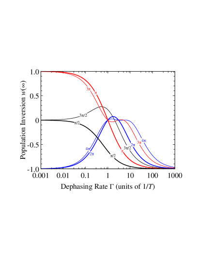
Figure 1: The population inversion, Eq. (17) for integer-$\pi$ pulses and Eq. (20) for half-integer-$\pi$ pulses, against the dephasing rate for different values of the pulse area $\mathcal{A}=\pi\alpha=\pi\Omega_{0}T$, denoted on the respective curve.

In Fig. 1 the population inversion $w(\infty)$ is plotted against the dephasing rate for different pulse areas.

III.2 Weak dephasing

When $\gamma\ll 1$ we use the relation $\Gamma(a+\gamma)=\Gamma(a)\left[1+\psi(a)\gamma+\mathcal{O}(\gamma^{2})\right]$, where $\psi(a)$ is the psi function, and the relation $\psi(1/2)=-\left(c+2\ln 2\right)$, where $c=0.5772156649\ldots$ is the Euler-Mascheroni constant AS ; Erdelyi . We thus find from Eq. (15) that

$$w(\infty) \approx -\left\{1-2\left[c+2\ln 2+\psi\left(\frac{1}{2}+\alpha\right)\right]\gamma+\mathcal{O}(\gamma^{2})\right\}$$ (21)

$$\times\cos\left[\pi\left(\alpha-\gamma\right)\right].$$

The first factor $\left\{\cdots\right\}$ describes the amplitude of the damped Rabi oscillations and the $\cos$ factor describes the phase of the oscillations. The maxima and the minima of these oscillations are shifted by $\pi\gamma$ (if the small additional shift from the damped amplitude is neglected) from their coherent values (6) and (7), respectively. The factor $\left\{\cdots\right\}$ in Eq. (21) displays explicitly the damping of the amplitude and its departure from 1 as $\gamma$ rises from zero. Since $\psi\left(\frac{1}{2}+\alpha\right)$ is an increasing function of $\alpha$ AS , the damping effect is stronger for larger pulse areas, which is shown explicitly below.

For $\alpha=\gamma+n$, near the $n$th extremum, we find from Eq. (21) by using Eq. (6.3.4) of AS for $\psi(n+\frac{1}{2})$ that

$$w(\infty)\approx\left(-1\right)^{n+1}\left[1-4\gamma\sum_{k=1}^{n}\frac{1}{2k-1}+\mathcal{O}(\gamma^{2})\right].$$ (22)

For $n=1-4$, Eq. (22) gives

$$n = 1:\quad w(\infty)\approx 1-4\gamma+\mathcal{O}(\gamma^{2}),$$ (23a)

$$n = 2:\quad w(\infty)\approx-1+\frac{16}{3}\gamma+\mathcal{O}(\gamma^{2}),$$ (23b)

$$n = 3:\quad w(\infty)\approx 1-\frac{92}{15}\gamma+\mathcal{O}(\gamma^{2}),$$ (23c)

$$n = 4:\quad w(\infty)\approx-1+\frac{704}{105}\gamma+\mathcal{O}(\gamma^{2}).$$ (23d)

The cases of $$n=1 \pi 3\pi n=2 2\pi 4\pi n\pi \pm 1 \gamma \gamma n$$ and 3 correspond to the first and second maxima ( and pulses), and and 4 to the first and second minima ( and pulses). Equations (22) and (23) show explicitly how the values of the population inversion for these pulses depart from their values as departs from zero. These equations also demonstrate that the effect of dephasing is stronger for larger pulse areas (since the coefficient in front of increases with ), which is indeed seen in Fig. 1.

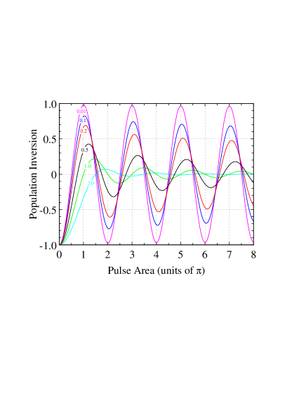
Figure 2: The population inversion (12) against the pulse area $\mathcal{A}=\pi\alpha$ for different values of the dephasing rate, $\Gamma T=0.01,0.1,$ $0.2,$ $0.5,1,2$ (denoted on the respective curve).

In Fig. 2 the population inversion is plotted against the pulse area for several values of the dephasing rate. As predicted, for $\gamma=\frac{1}{2}$ ($\Gamma T=1$), the nodes of $w$ are situated at pulse areas $\mathcal{A}=n\pi$, where in the absence of dephasing one finds the extrema. For $\gamma=1$ ($\Gamma T=2$), the maxima are situated approximately at $\alpha=2,4,6,\ldots$, where one finds the minima (even-$\pi$ pulses) for $\gamma=0$; likewise, the minima are situated approximately at $\alpha=3,5,7,\ldots$, where one finds the maxima (odd-$\pi$ pulses) for $\gamma=0$.

III.3 Strong dephasing

For $\gamma\gg\alpha,1$, the population inversion $w(\infty)$ has the asymptotics

$$w(\infty)\sim-\exp\left[-\frac{\alpha^{2}}{\gamma}+\mathcal{O}(\gamma^{-3})\right],$$ (24)

which is obtained from Eq. (12) by using the Stirling asymptotic expansion AS ,

$$\Gamma(z) \sim \sqrt{2\pi}z^{z-\frac{1}{2}}\exp\left[-z+\frac{1}{12z}+\mathcal{O}\left(\left|z\right|^{-3}\right)\right],$$

$$\qquad\left(\left|\arg z\right|<\pi,\left|z\right|\gg 1\right).$$

The inversion $w(\infty)$ decreases in a Gaussian fashion against $\alpha$. For large $\gamma$, $w$ tends to its initial value of $-1$, rather than to the incoherent limit $w=0$, which is a result of quantum overdamping Vitanov97 . This behavior is indeed seen in Fig. 1, where we have verified that Eq. (24) describes very accurately the asymptotic decrease of $w(\infty)$ for large $\gamma$ (not shown for simplicity).

III.4 Large pulse area

When $\alpha\gg\gamma,1$, the population inversion $w(\infty)$ has the following behavior

$$w(\infty)\sim-\frac{1}{\pi}\Gamma^{2}\left(\frac{1}{2}+\gamma\right)\alpha^{-2\gamma}\left[1+\mathcal{O}(\alpha^{-2})\right]\cos\pi(\alpha-\gamma),$$ (26)

which is derived from Eq. (15) by using Eq. (III.3). Equation (26) shows that as $\alpha$ increases, the oscillation amplitude vanishes as $\alpha^{-2\gamma}$ and for sufficiently large pulse areas,

$$\mathcal{A}\gtrsim\mathcal{A}_{\varepsilon}=\pi\left[\frac{\pi\varepsilon}{\Gamma^{2}\left(\frac{1}{2}+\gamma\right)}\right]^{-\frac{1}{2\gamma}},$$ (27)

the population inversion decreases below $\varepsilon$ ($\left|w\right|\lesssim\varepsilon$), i.e. the two-state system evolves towards a completely incoherent superposition of states $\left|1\right\rangle$ and $\left|2\right\rangle$ ($\rho_{11}=\rho_{22}=\frac{1}{2}$, $\rho_{12}=0$). For instance, $\mathcal{A}_{0.1}\approx 1.58\times 10^{9}\pi$, $415\pi$, and $3.18\pi$ for $\gamma=0.1$, $0.3$, and $1$, respectively.

IV Conclusions

In this paper we have presented an exact analytic solution for resonant excitation induced by a pulse with a hyperbolic-secant shape in the presence of dephasing processes. The exact solution (12) is given in terms of gamma functions. Dephasing affects the Rabi oscillations in two ways: shifting the oscillation phase by approximately $\pi\Gamma T/2$ and damping the oscillation amplitude: the larger the pulse area, the stronger the damping. The implication is that one cannot reduce the dephasing-induced losses of efficiency by increasing the intensity of the field (e.g. replacing a $\pi$ pulse by a $3\pi$ pulse) since this will actually increase the losses.

Various special cases of pulses with specific areas have been considered and various limits have been derived in terms of elementary functions. The results provide explicit and simple estimates of the effect of dephasing on resonant excitation, e.g. in the cases of $\pi$, $2\pi$ and $\pi/2$ pulses, which are of great importance and widely used in many fields.

Acknowledgements

This work has been supported by the EU Transfer of Knowledge project CAMEL, the Alexander von Humboldt Foundation, and the EU Research and Training Network QUACS (HPRN-CT-2002-00309).

Appendix A Exact solution

The first step in solving Eqs. (11) is to decouple them by differentiating the equation for $\dot{w}$ and replacing $v$ and $\dot{v}$, found from Eqs. (11); this gives

$$\ddot{w}-\left(\Gamma+\frac{\dot{\Omega}}{\Omega}\right)\dot{w}+\Omega^{2}w=0,$$ (28)

with an overdot denoting $d/dt$. We change the independent variable from $t$ to $z(t)=\frac{1}{2}[\tanh(t/T)+1]$; hence $z(-\infty)=0$ and $z(+\infty)=1$. Then

$$z(1-z)W^{\prime\prime}+\left(\frac{1}{2}+\gamma-z\right)W^{\prime}+\alpha^{2}W=0,$$ (29)

where ${}^{\prime}\equiv d/dz$, $W\left[z(t)\right]=w(t)$ and $\alpha$ and $\gamma$ are defined by Eqs. (13). This equation has the same form as the Gauss hypergeometric equation AS ; GR ,

$$z(1-z)F^{\prime\prime}+\left[\nu-(\lambda+\mu+1)z\right]F^{\prime}-\lambda\mu F=0,$$ (30)

upon the identification

$$\lambda=\alpha,\qquad\mu=-\alpha,\qquad\nu=\frac{1}{2}+\gamma.$$ (31)

The complete solution of this equation, expressed by a superposition of two linearly independent solutions of Eq. (29), depends upon the value of $\nu$.

The case $\nu\neq 1,2,3,\ldots$According to Sec. 9.153.1 of GR , the solution of Eq. (29) can be expressed in terms of the Gauss hypergeometric function AS ; GR as

$$W(z) = A_{1}F(\lambda,\mu;\nu;z)$$ (32)

$$+A_{2}z^{1-\nu}F(\lambda+1-\nu,\mu+1-\nu;2-\nu;z).$$

From here and using Eq. (11), it can be found that

$$V(z) = \frac{i\sqrt{z(1-z)}}{\alpha}\bigg{[}A_{1}\frac{\lambda\mu}{\nu}F(\lambda+1,\mu+1;\nu+1;z)$$ (33)

$$+ A_{2}(1-\nu)z^{-\nu}F(\lambda+1-\nu,\mu+1-\nu;1-\nu;z)\bigg{]},$$

with $V[z(t)]=v(t)$, where Eqs. (15.2.1) and (15.2.4) of AS have been used. The integration constants $A_{1}$ and $A_{2}$ can be determined from the initial conditions (2),

$$A_{1}=-1,\qquad A_{2}=0.$$ (34)

Hence $w(\infty)=W(1)=-F(\lambda,\mu;\nu;1)$ or

$$w(\infty)=-\frac{\Gamma(\nu)\Gamma(\nu-\lambda-\mu)}{\Gamma(\nu-\lambda)\Gamma(\nu-\mu)},$$ (35)

where Eq. (15.1.20) of AS has been used. Referring to Eqs. (31), one obtains Eq. (12).

Equation (35) has been derived under the assumption that $\nu\neq 1,2,3,\ldots$; then the two terms in Eq. (32) are linearly independent. Suppose now that $\nu=n$ where $n=1,2,3,\ldots$, that is $\gamma=\frac{1}{2},\frac{3}{2},\frac{5}{2},\ldots$; Then the two terms in Eq. (32) are linearly dependent for $\nu=1$ while the second term is not defined for $\nu=2,3,4,\ldots$

The case $\nu=1$. According to Sec. 9.153.2 of GR , the solution of Eq. (29) for $\nu=1$ is

$$W(z) = A_{1}F(\lambda,\mu;1;z)$$ (36)

$$+ A_{2}\left[F(\lambda,\mu;1;z)\ln z+\sum_{k=1}^{\infty}\frac{(\lambda)_{k}(\mu)_{k}\psi_{1}}{(k!)^{2}}z^{k}\right],$$

with $(x)_{k}=\Gamma(x+k)/\Gamma(x)$ and $\psi_{1}=\psi(\lambda+k)-\psi(\lambda)+\psi(\mu+k)-\psi(\mu)-2\psi(k+1)+2\psi(1)$, $\psi(x)$ being the psi-function AS . Since the second term diverges for $z=0$, the initial conditions (2) require Eqs. (34) to be satisfied and Eq. (35) applies again.

The case $\nu=n+1$ $(n=1,2,3,\ldots)$ and $\lambda,\mu\neq 0,1,2,\ldots,n-1$. According to Sec. 9.153.3 of GR and Eq. (15.5.19) of AS , the solution of Eq. (29) in this case is

$$W(z) = A_{1}F(\lambda,\mu;n+1;z)+A_{2}\bigg{[}F(\lambda,\mu;n+1;z)\ln z$$ (37)

$$+ \sum_{k=1}^{\infty}\frac{(\lambda)_{k}(\mu)_{k}\psi_{n+1}}{(n+1)_{k}k!}z^{k}-\sum_{k=1}^{n}\frac{(k-1)!(-n)_{k}}{(1-\lambda)_{k}(1-\mu)_{k}}z^{-k}\bigg{]}$$

with $\psi_{n+1}=\psi(\lambda+k)-\psi(\lambda)+\psi(\mu+k)-\psi(\mu)-\psi(n+1+k)+\psi(n+1)-\psi(1+k)+\psi(1)$. Again, the second term diverges for $z=0$ and the initial conditions (2) require Eqs. (34) to be satisfied and hence, Eq. (35) holds again.

The case $\nu=n+1$ $(n=1,2,3,\ldots)$ and $\lambda$ or $\mu=0,1,2,\ldots,n-1$. Suppose that $\lambda=m+1<n+1$. Then, according to Sec. 9.153.4 of GR , the solution is given by Eq. (32), in which the second hypergeometric function reduces to a polynomial in $z^{-1}$. Since it diverges for $z=0$, the initial conditions (2) require Eqs. (34) to be satisfied and Eq. (35) holds again.

In conclusion, for the model (3), in all cases the final population inversion $w(+\infty)$ is given by Eq. (35).

References

- (1) B. W. Shore, The Theory of Coherent Atomic Excitation (Wiley, New York, 1990).
- (2) L. Allen and J. H. Eberly, Optical Resonance and Two-Level Atoms (Dover, New York, 1987).
- (3) N.V. Vitanov, M. Fleischhauer, B.W. Shore, and K. Bergmann, Coherent manipulation of atoms and molecules by sequential laser pulses, in Adv. At. Mol. Opt. Phys., ed. B. Bederson and H. Walther (Academic, New York, 2001), vol. 46, pp. 55-190; N.V. Vitanov, T. Halfmann, B.W. Shore, and K. Bergmann, Ann. Rev. Phys. Chem. 52, 763 (2001).
- (4) N. Rosen and C. Zener, Phys. Rev. 40, 502 (1932).
- (5) N. V. Vitanov, J. Phys. B 31, 709 (1998).
- (6) N. V. Vitanov and S. Stenholm, Phys. Rev. A 55, 2982 (1997).
- (7) A. Erdélyi, W. Magnus, F. Oberhettinger, and F. G. Tricomi, Higher Transcendental Functions, vol.II (McGraw-Hill, New York, 1953).
- (8) M. Abramowitz and I. A. Stegun (editors), Handbook of Mathematical Functions (Dover, New York, 1964).
- (9) I. S. Gradsteyn and I. M. Ryzhik, Table of Integrals, Series, and Products (Academic Press, New York, 1980).