On the galaxy stellar mass function, the mass-metallicity relation, and the implied baryonic mass function

Abstract

A comparison between published field galaxy stellar mass functions (GSMFs) shows that the cosmic stellar mass density is in the range 4–8 per cent of the baryon density (assuming $\Omega_{b}=0.045$). There remain significant sources of uncertainty for the dust correction and underlying stellar mass-to-light ratio even assuming a reasonable universal stellar initial mass function. We determine the $z<0.05$ GSMF using the New York University – Value-Added Galaxy Catalog sample of 49968 galaxies derived from the Sloan Digital Sky Survey and various estimates of stellar mass. The GSMF shows clear evidence for a low-mass upturn and is fitted with a double Schechter function that has $\alpha_{2}\simeq-1.6$. At masses below $\sim 10^{8.5}{\cal M}_{\odot}$, the GSMF may be significantly incomplete because of missing low surface-brightness galaxies. One interpretation of the stellar mass-metallicity relation is that it is primarily caused by a lower fraction of available baryons converted to stars in low-mass galaxies. Using this principal, we determine a simple relationship between baryonic mass and stellar mass and present an ‘implied baryonic mass function’. This function has a faint-end slope, $\alpha_{2}\simeq-1.9$. Thus, we find evidence that the slope of the low-mass end of the galaxy mass function could plausibly be as steep as the halo mass function. We illustrate the relationship between halo baryonic mass function $\rightarrow$ galaxy baryonic mass function $\rightarrow$ GSMF. This demonstrates the requirement for peak galaxy formation efficiency at baryonic masses $\sim 10^{11}{\cal M}_{\odot}$ corresponding to a minimum in feedback effects. The baryonic-infall efficiency may have levelled off at lower masses.

1 Introduction

The galaxy luminosity or mass function is a fundamental tool used in interpreting the evolution of galaxies. The functions are usually defined as the number density of galaxies per logarithmic luminosity or mass interval. A steeply rising mass function to the faint population has been a generic prediction of galaxy formation based on hierarchical clustering (White & Rees, 1978; Kauffmann et al., 1993; Cole et al., 1994). In contrast, the field galaxy luminosity function was observed to have a significantly flatter ‘faint end’ (Binggeli et al., 1988; Loveday et al., 1992). In order to reconcile cold dark matter (CDM) galaxy formation models with the observed luminosity function, star formation (SF) is suppressed in low-mass halos by, for example, supernovae feedback (Lacey & Silk, 1991; Kay et al., 2002) or photoionisation (Efstathiou, 1992; Somerville, 2002).

On the observational side, accurately determining the number densities of faint galaxies in the field or in clusters is challenging. This is mainly because of the low surface brightness (SB) of these galaxies, which means that they can be undetected in photometry even if high-SB galaxies with the same apparent magnitude are detected (Disney, 1976; Disney & Phillipps, 1983). Despite these and other challenges, there is evidence for a ‘faint-end upturn’ in luminosity functions whereby the luminosity function is rising steeply fainter than about 3–5 magnitudes below the characteristic luminosity, in clusters (Driver et al., 1994; Popesso et al., 2005) or the field (Loveday, 1997; Zucca et al., 1997; Marzke et al., 1998; Blanton et al., 2005a). Note however that the upturn is not always evident (Norberg et al., 2002; Harsono & de Propris, 2007).

A faint-end upturn suggests that the efficiency of feedback has levelled off at low galaxy luminosities. A more direct analysis is to compare galaxy mass functions with predicted mass functions from CDM models. Klypin et al. (1999) compared the circular velocity distribution of satellite galaxies in the Local Group (see also Moore et al. 1999). This highlights the ‘substructure problem’ where there are 5–10 times as many low-mass satellites in CDM models than observed. However, we still have not reached a complete census of Local Group satellites as evidenced by recent discoveries of low-SB galaxies around M31 (Martin et al., 2006) and the Milky Way (Belokurov et al., 2007).

Reliable dynamical mass estimates for complete and large samples of field galaxies are difficult to obtain. Stellar masses can be estimated for significantly larger samples of galaxies using the principles of stellar population synthesis (Tinsley & Gunn, 1976; Tinsley, 1980). Thus, galaxy stellar mass functions (GSMFs) can be derived from galaxy luminosities (e.g., Balogh et al. 2001; Cole et al. 2001; Bell et al. 2003b; Kodama & Bower 2003). Comparisons between GSMFs are then, in theory, free of the stellar-population contribution to mass-to-light (M-L) variations that are inherent in comparisons between luminosity functions.

Integrating a field GSMF to determine the cosmic stellar mass density (SMD) brings to light the large gap between this value ($\Omega_{\rm stars}\sim 0.003$) and estimates of $\Omega_{b}$ from Big-Bang Nucleosynthesis theory (0.04, Burles, Nollett, & Turner 2001) or the power spectrum of the cosmic background radiation (0.045, Spergel et al. 2007). Even determination of the baryonic content of galaxies including stars and cold gas accounts for less than or about 0.1 of $\Omega_{b}$ (Bell et al., 2003a). About 0.2 of $\Omega_{b}$ is accounted for by hot plasma identified by X-ray emission in clusters and groups (Fukugita, Hogan, & Peebles, 1998); while the rest is projected to be in a more diffuse inter-galactic medium (Cen & Ostriker, 1999) and perhaps the ‘coronae’ of galaxies (Maller & Bullock, 2004). The overall efficiency of baryons falling into the luminous disks or bulges of galaxies is low.

The efficiency of SF (fraction of baryonic mass converted to stars) varies significantly with galaxy mass. A low efficiency averaged over the life of a galaxy gives rise to a low gas-phase metallicity (in the inter-stellar medium) because the metal production by supernovae is diluted by gas reservoirs within a galaxy (Tinsley, 1980; Brooks et al., 2007) and further infalling material. Conversely a high efficiency can drive the gas-phase metallicity to high values. In this paper, we explore the use of the stellar mass-metallicity relation (Tremonti et al., 2004) as a SF efficiency estimator to convert the GSMF to a baryonic mass function.

The plan of this paper follows. Determinations of the field GSMF and the SMD are reviewed in § 2. An estimate of the low-redshift field GSMF paying careful attention to SB selection effects is described in § 3. The evident faint-end upturn is compared with cluster GSMFs. The relationship between gas-phase metallicity and stellar mass is then used to convert the field GSMF to an ‘implied baryonic mass function’ assuming a simple relationship between metallicity and the fraction of baryonic mass in stars. This is described in § 4. This galaxy baryonic mass function, and the GSMF, are compared with halo mass functions and related to galaxy formation efficiency as a function of mass. Summary and conclusions are presented in § 5. The dependencies of stellar M-L ratio on various assumptions are presented in the Appendix. Throughout this paper, a cosmology with $H_{0}=70{\rm\,km\,s^{-1}\,Mpc^{-1}}$, $\Omega_{m,0}=0.3$ and $\Omega_{\Lambda,0}=0.7$ is assumed.

2 Comparison between published galaxy stellar mass functions

By estimating stellar M-L ratios for galaxies it is possible to calculate the equivalent of a luminosity function, for the total stellar mass of galaxies, known as the galaxy stellar mass function (Cole et al., 2001). This then gives a more fundamental account of the baryons that are locked up in stars and how they are distributed amongst galaxies of different masses.

One of the key ingredients in this calculation is the stellar initial mass function (IMF), which is generally assumed to be independent of galaxy type or mass (Elmegreen, 2001). For the comparisons in this paper, the IMFs used are the ‘diet Salpeter’ that is defined as $0.7\,\times$ the mass derived from a standard Salpeter (Bell & de Jong, 2001; Bell et al., 2003b), the Kroupa (2001), and the Chabrier (2003) IMF. These are all similar in terms of M-L ratio as a function of galaxy colour. The variations highlighted and discussed between different mass estimates in this paper are not significantly dependent on IMF choice (Appendix).

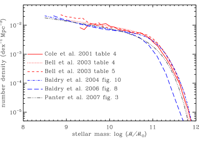
Figure 1 shows a comparison between published field GSMFs (where ‘field’ in this case means a cosmic volume average). A brief description of how these were derived is given below. Masses and number densities were converted to a cosmology with $H_{0}=70{\rm\,km\,s^{-1}\,Mpc^{-1}}$ where necessary.

Figure 1: Comparison between published field galaxy stellar mass functions ($z\la 0.1$). The mass functions have been converted to $H_{0}=70{\rm\,km\,s^{-1}\,Mpc^{-1}}$ where necessary and the Cole et al. GSMF has been converted to the diet Salpeter IMF.

1. Cole et al. (2001): data were taken from the Salpeter column of table 4. The masses were multiplied by 0.7 to convert to the diet Salpeter IMF. The published GSMF was derived from a match of the Two Micron All Sky Survey (2MASS) extended source catalogue (Jarrett et al., 2000) to the 2dF Galaxy Redshift Survey (2dFGRS; Colless et al. 2001). Cole et al. computed $b_{J}-K$ and $J-K$ colours for a range of exponentially declining SF histories with $z_{\rm form}=20$ and metallicities using Bruzual & Charlot (1993) models. Dust attenuation from the models of Ferrara et al. (1999) were applied. Stellar M-L ratios in the near-IR bands were determined from the models that most closely matched the observed galaxies’ colours; with stellar masses assumed to be 0.72 times the integral of the SF rate (to account for recycling).

2. Bell et al. (2003b): data were taken from table 4. The plotted GSMF is the sum of the $g$-band derived early- and late-type Schechter functions. The GSMFs were derived from a match of the 2MASS catalogue to the Sloan Digital Sky Survey (SDSS; York et al. 2000; Stoughton et al. 2002). The $ugrizK$ data were fitted to magnitudes computed for a range of exponential SF histories and metallicities using PEGASE (Fioc & Rocca-Volmerange, 1997, 1999) models. M-L ratios were determined from the best-fit models.

3. Bell et al.: as above but using data taken from table 5. This is a binned GSMF derived from the same M-L ratios.

4. Baldry et al. (2004): data were taken from fig. 10. The GSMF is the sum of the red- and blue-sequence Schechter functions. This was derived from SDSS data with a M-L ratio given by a linear function of colour: $\log({\cal M}/{L_{r}})\>=\>-0.55\,+\,0.45\,(u-r)\,$. This relation was determined from stellar masses computed by Bell et al. (2003b) and Kauffmann et al. (2003).

5. Baldry et al. (2006): data were taken from fig. 8. The GSMF is the sum over all the environments. This was derived in a similar way to that of Baldry et al. (2004) using a different relationship between M-L ratio and colour. In this case, the relation was determined from stellar masses computed by Kauffmann et al. (2003) and K.G. These methods are described in § 3.

6. Panter et al. (2007): data were taken from fig. 3. The GSMF is derived from the Schechter parameters. The method for estimating stellar masses is described in § 3.

The GSMFs are similar except for the Baldry et al. (2006) function, which appears to be shifted by about 0.2 dex to lower masses. This is because the method used by K.G. for that paper underestimated the masses of luminous red galaxies. This may reflect degeneracies with fitting to only $ugriz$ photometry and attempting to fit SF bursts, metallicity and dust attenuation (Appendix).

2.1 The stellar mass density of the Universe

A quantitative overall comparison can be made by integrating each GSMF to obtain the total SMD. The critical density for $H_{0}=70{\rm\,km\,s^{-1}\,Mpc^{-1}}$ is $\rho_{c}=1.36\times 10^{11}{\cal M}_{\odot}{\rm Mpc}^{-3}$ and we assume $\Omega_{b}=0.045$ (Spergel et al., 2007). The fraction of baryons in stars $f_{s}=\Omega_{\rm stars}/\Omega_{b}$ is then (i) 0.054, (ii) 0.061, (iii) 0.063, (iv) 0.056, (v), 0.035, (vi) 0.042. Note these values do not include extrapolations of the GSMF to lower masses than the plotted points or corrections to total galaxy magnitudes from catalogue magnitudes unless already applied.

The total SMD can also be determined using methods other than integrating a GSMF. Driver et al. (2007) determined $f_{s}=0.083\pm 0.012$ from the $B$-band luminosity function using an empirical geometrical-based correction for dust attenuation; Baldry & Glazebrook (2003) give a range from 0.035 to 0.063 from fitting to the local cosmic luminosity densities (over a range of IMFs but similar to those used here in terms of M-L ratio); and Nagamine et al. (2006) found $0.051\pm 0.009$ from fitting to various data including the extragalactic background light. See also table 5 of Gallazzi et al. (2008) for a list of SMD measurements.

Overall there remains a considerable uncertainty in $\Omega_{\rm stars}$ or $f_{s}$, which is probably in the range 4–8 per cent (for the Chabrier, Kroupa or diet Salpeter IMF). This is much larger than the uncertainty in $\Omega_{m}$ or $\Omega_{b}$ within the standard cosmological paradigm.

Accounting for dust is obviously a major problem. Correcting for attenuation by incorporating a dust law in stellar population synthesis (PS) models, and fitting to colours and/or spectral features, cannot account for populations behind opaque screens. Notably, Driver et al. (2007) obtain the largest value of $f_{s}$ and the method uses comparisons of disks and bulges viewed at various orientations to constrain their dust model (Tuffs et al., 2004). It is then useful to compare the SMD with near-IR measurements that are minimally affected by dust attenuation. The total $K$-band luminosity density, in units of $10^{8}L_{\odot}{\rm Mpc}^{-3}$, is given by 4.0 (Cole et al., 2001), 5.0 (Kochanek et al., 2001) and 4.1 (Bell et al., 2003b). Using these values and the full range of $f_{s}=0.035$–0.083 implies a cosmic $\log({\cal M}/{L_{K}})$ in the range $-0.35$ to $0.1$. A high SMD with $f_{s}\sim 0.08$ appears unlikely given that only the oldest simple stellar populations have $\log({\cal M}/{L_{K}})\simeq 0.0$ (Appendix); unless there is more than nominal attenuation of the $K$-band and/or the $K$-band luminosity density is underestimated.

How can we reconcile the Driver et al. (2007) result ($0.083\pm 0.012$) with the standard PS methods of Fig. 1 (0.04–0.06 ignoring extremes) other than resorting to saying the higher result is 2-sigma too high? The standard PS methods cannot account for populations behind optically-thick screens and use less deep photometry than the Driver et al. result, which is based on the Millennium Galaxy Catalogue (MGC). A reasonable estimate of unaccounted for light would be 20% bringing $f_{s}$ up to 0.05–0.07 for the standard PS methods. On the other hand, the MGC estimate is subject to larger cosmic variance and the luminosity density appears to be high by 10–20%, and the M-L ratios assumed for the attenuation-corrected magnitudes could also be high by 10%. Accounting for these brings $f_{s}$ down to 0.06–0.07 in agreement with the standard PS methods.

While the largest contribution to the SMD comes from galaxies around the break in the GSMF, lower mass galaxies play a key role in the processing of baryons. In the next section, we discuss a new calculation of GSMFs using various stellar mass estimates and consider how accurately the lower-mass end can be determined.

3 Galaxy stellar mass functions from the NYU-VAGC low redshift galaxy sample

A large low-redshift sample derived from the SDSS is the New York University – Value-Added Galaxy Catalog (NYU-VAGC) (Blanton et al., 2005a, b). While the data are obtained from standard SDSS catalogues, the images have been carefully checked for artifacts including deblending. The data cover cosmological redshifts from 0.0033 to 0.05 where the redshifts have been corrected for peculiar velocities using a local Hubble-flow model (Willick et al., 1997). We use the NYU-VAGC low-$z$ galaxy sample to recompute the GSMF down to low masses.

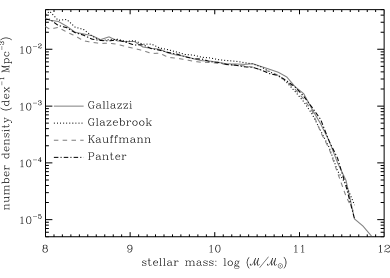
The Data Release Four (DR4) version of the NYU-VAGC low-$z$ sample includes data for 49968 galaxies. These data were matched to stellar masses estimated by Kauffmann et al. (2003), Gallazzi et al. (2005), and Panter et al. (2007); with 49473, 32473 and 38526 matches, respectively. Minor adjustments were determined to account for variations between the SDSS data from which the stellar masses were determined and the NYU-VAGC (photometry and cosmological redshifts). Where no stellar mass was available for a galaxy, the stellar mass was determined using a colour-M-L relation calibrated to the particular set of stellar masses. In addition, stellar masses were computed by K.G. using the NYU-VAGC Petrosian magnitudes. Thus there are four stellar masses for each galaxy. The methods are described briefly below.

1. Kauffmann: The stellar masses were obtained by fitting a grid of population synthesis models, including bursts, to the spectral features D4000 and H$\delta$ absorption. The predicted colours were then compared with broad-band photometry to estimate dust attenuation. Stellar M-L ratios were determined and applied to the Petrosian $z$-band magnitude. For details see Kauffmann et al. (2003).

2. Gallazzi: The computation was similar to the above method except five spectral features were used. The features were carefully chosen for calculating stellar metallicity and light-weighted ages while minimising effects caused by chemical abundance ratios. For details see Gallazzi et al. (2005).

3. Panter: The computation involves fitting synthetic stellar populations to each galaxy spectrum using the MOPED data compression technique (Heavens, Jimenez, & Lahav, 2000). The SF history of each galaxy was modelled using 11 logarithmically-spaced bins in time, each with an SF rate and metallicity, and a simple dust screen. The total stellar mass is that obtained from the Bruzual & Charlot (2003) models given the best-fitting SF history as input. For details see Panter et al. (2004, 2007) and references therein.

4. Glazebrook: This is the only purely photometric method. Stellar masses were determined by fitting to the observed-frame Petrosian $ugriz$ magnitudes of each galaxy. A grid of colours were computed using PEGASE models. A range of exponential SF histories and metallicities were input. Bursts were added with mass ranging from $10^{-4}$ to twice the mass of the primary component (Glazebrook et al., 2004). For this paper, no dust attenuation was included in the models (see Appendix for discussion). Depending on the attenuation law, incorporating dust can be close to neutral in terms of M-L ratio versus colour (Bell & de Jong 2001; see fig. 12 of Driver et al. 2007 for the effect modelled from face-on to edge-on).

The IMFs used were the similar Kroupa and Chabrier IMFs, for methods (i,iv) and methods (ii,iii), respectively. Comparing the different mass estimates for each galaxy, the standard deviation is typically in the range 0.05–0.15 dex. The standard deviation is generally lower for red-sequence galaxies compared to blue-sequence galaxies.

For each set of stellar masses, the galaxies were divided into logarithmic stellar mass bins. For each bin, the GSMF is then given by

$$\phi_{\log{\cal M}}=\frac{1}{\Delta\log{\cal M}}\,\sum_{i}\frac{1}{V_{{\rm max},i}}w_{i}$$ (1)

where: $V_{{\rm max},i}$ is the comoving volume over which the $i$th galaxy could be observed, and $w_{i}$ is any weight applied to the galaxy. The $V_{\rm max}$ values were obtained from the NYU-VAGC catalogue (§ 5 of Blanton et al. 2005b). Figure 2 shows the GSMFs derived from the NYU-VAGC using the different stellar mass estimates. For these, no weighting was applied to any galaxy ($w=1$).

Figure 2: Comparison between galaxy stellar mass functions derived from the NYU-VAGC low-$z$ galaxy sample. The lines represent different methods of determining M-L ratios from spectra or colours. The functions were determined by summing $1/V_{\rm max}$ in logarithmic mass bins.

While all the GSMFs are relatively similar, they all show a subtle ‘dip’ relative to a smooth slope around $10^{8.6}{\cal M}_{\odot}$ in Fig. 2. This feature is a product of using $1/V_{\rm max}$ with large-scale structure (LSS) variations (Efstathiou, Ellis, & Peterson, 1988). Figure 3 shows how the number density of a volume-limited sample of galaxies ($M_{r}<-19$) varies with redshift. There is a clear underdensity around $z\sim 0.013$ that is the cause of the GSMF dip. See also Blanton et al. (2005a), e.g. fig. 9 of that paper, for the effect of this LSS on the luminosity function. A simple way of removing this effect is to set $w_{i}$, for each galaxy, equal to $1/n(z)$ where $n$ is the normalised number density as shown in Fig. 3 at the redshift of the galaxy. Before recomputing the GSMF in this way, we discuss the selection limits related to surface brightness and M-L ratio. The mass used for each galaxy in the rest of the paper is obtained from the mean of the $\log{\cal M}$ estimates.

Figure 3: LSS fluctuations in the low-$z$ galaxy sample. The solid line shows the relative number density of galaxies brighter than $M_{r}=-19$ in redshift shells. The number densities were normalised by the volume average over $z<0.05$. The dashed and dotted lines show the normalised densities for $M_{r}<-20.0$ and $-21.0$, respectively, from the DR4 sample of Baldry et al. (2006). The dash-and-dotted lines show the volume averages for $z<0.05$ ($=1$ by design) and $z<0.1$ ($=1.13$).

3.1 Selection limits

One of the key factors in considering the determination of the GSMF is the SB limit, which is often not explicitly identified, of a redshift survey (Cross & Driver, 2002). From the tests of Blanton et al. (2005a), as shown in fig. 3 of that paper, the SDSS main galaxy sample has 70% or greater completeness in the range 18–$23{\rm\,mag\,arcsec}^{-2}$ for the effective SB $\mu_{R50,r}$.

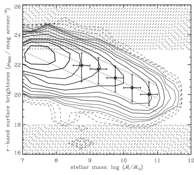
In order to identify at what point the GSMF becomes incomplete because of the SB limit we computed the bivariate distribution in SB versus stellar mass. Figure 4 shows this distribution represented by solid and dashed contours ($1/V_{\rm max}$ and $1/n$ LSS corrected). There is a relationship between peak SB and $\log{\cal M}$, which is approximately linear in the range $10^{8.5}$ to $10^{11}{\cal M}_{\odot}$. At lower masses, the distribution is clearly affected by the low SB incompleteness at $\mu_{R50,r}>23{\rm\,mag\,arcsec}^{-2}$. Therefore, any GSMF values for lower masses should be regarded as lower limits if there are no corrections for SB completeness.

Figure 4: Bivariate distribution for SB versus mass. The contours represent the volume-corrected number densities from the sample: logarithmically spaced with four contours per factor of ten. The lowest dashed contour corresponds to $10^{-5}{\rm\,Mpc}^{-3}$ per $0.5\times 0.5$ bin, while the lowest solid contour corresponds to $5.6\times 10^{-5}{\rm\,Mpc}^{-3}$. The grey dashed-line regions represent areas of low completeness (70% or lower as estimated by Blanton et al. 2005a). The diamonds with error bars represent the median and 1-sigma ranges over certain masses with a straight-line fit shown by the middle dotted line. The outer dotted lines represent $\pm 1$ sigma.

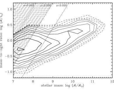
The other important consideration is fact that the $r$-band selection is not identical to the mass selection required for the GSMF. This is nominally corrected for by $1/V_{\rm max}$ but it should be noted that galaxies with high M-L ratio at a given mass are viewed over significantly smaller volumes than those with low M-L ratio. Figure 5 shows the bivariate distribution in M-L ratio versus mass. The limits at various redshifts for the SDSS main galaxy sample are also identified. For example, galaxies with ${\cal M}<10^{8}{\cal M}_{\odot}$ and $\log({\cal M}/L_{r})>0.1$ are only in the sample at $z<0.008$. At these low redshifts, the stellar mass and $V_{\rm max}$ depend significantly on the Hubble-flow corrections. However, it does appear that the SB limit affects the completeness of GSMF values at higher masses than the M-L limits. At ${\cal M}<10^{8.5}{\cal M}_{\odot}$ the SB limit becomes significant, while at ${\cal M}<10^{8}{\cal M}_{\odot}$, the GSMF is affected both by the constrained volume for high M-L ratio galaxies and more severely by the SB incompleteness.

Figure 5: Bivariate distribution for M-L ratio versus mass. The contours represent the volume-corrected number densities: logarithmically spaced with four contours per factor of ten. The lowest dashed contour corresponds to $10^{-4}{\rm\,Mpc}^{-3}$ per $0.5\times 0.2$ bin. The dotted lines represent the observable limits for an $r<17.8$ magnitude limit and different redshift limits (ignoring k-corrections). The grey dashed-line region represents galaxies that can only be observed at $z<0.008$ where Hubble-flow corrections are significant ($cz<2400{\rm\,km\,s}^{-1}$).

3.2 Corrected GSMF with lower limits at the faint end

Figure 6 shows the results of the GSMF determination. The binned GSMF is represented by points with Poisson error bars, with lower limits represented by arrows. The GSMF has been corrected for volume ($1/V_{\rm max}$) and LSS ($1/n$) effects. The masses used were the average of the four estimated stellar masses. The shaded region represents the full range in the GSMF obtained by varying the stellar mass used (Fig. 2) and multiplying the upper number densities by 1.13 to account for the expected renormalisation at $z<0.1$ (Fig. 3). After renormalisation, the range in $f_{s}$ is 0.038–0.048. In addition if we multiply by 1.2 to account for missing light (optically-thick regions and corrections to total magnitudes, § 2), we obtain 0.046–0.058.

Figure 6: GSMF extending to down to $10^{7}{\cal M}_{\odot}$ determined from the NYU-VAGC. The points represent the non-parametric GSMF with Poisson error bars; at ${\cal M}<10^{8.5}{\cal M}_{\odot}$ the data are shown as lower limits because of the SB incompleteness (Fig. 4). The dashed line represents a double-Schechter function extrapolated from a fit to the ${\cal M}>10^{8}{\cal M}_{\odot}$ data points. The dotted line shows the same type of function with a faint-end slope of $\alpha_{2}=-1.8$ (fitted to ${\cal M}>10^{8.5}{\cal M}_{\odot}$ data). The dash-and-dotted line represents a power-law slope of $-2.0$. The shaded region shows the range in the GSMF from varying the stellar mass used and changing the redshift range.

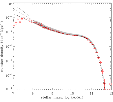
The binned data for the GSMF can clearly not be represented by a single Schechter (1976) function. The data were fitted with a double Schechter function given by

$$\phi_{\cal M}\,{\rm d}{\cal M}=e^{-{\cal M}/{\cal M}^{*}}\left[\phi^{*}_{1}\left(\frac{{\cal M}}{{\cal M}^{*}}\right)^{\alpha_{1}}+\phi^{*}_{2}\left(\frac{{\cal M}}{{\cal M}^{*}}\right)^{\alpha_{2}}\right]\,\frac{{\rm d}{\cal M}}{{\cal M}^{*}}$$ (2)

where $\phi_{\cal M}\,{\rm d}{\cal M}$ is the number density of galaxies with mass between ${\cal M}$ and ${\cal M}+{\rm d}{\cal M}$; with $\alpha_{2}<\alpha_{1}$ so that the second term dominates at the faintest magnitudes. Fitting to ${\cal M}>10^{8}{\cal M}_{\odot}$, the best-fit parameters are

$$\begin{array}[]{ll}\log({\cal M}^{*}/{\cal M}_{\odot})=10.648\\ \phi^{*}_{1}/10^{-3}{\rm\,Mpc}^{-3}=4.26&\alpha_{1}=-0.46\\ \phi^{*}_{2}/10^{-3}{\rm\,Mpc}^{-3}=0.58&\alpha_{2}=-1.58\end{array}$$ (3)

with formal errors of 0.013, 0.09, 0.05, 0.07, 0.02. The dashed line in Fig. 6 represents this fit extrapolated down to $10^{7}{\cal M}_{\odot}$.

Even though the Poisson errors are small, for illustrative purposes and because systematic errors are clearly significant, we fitted a function with $\alpha_{2}=-1.8$ fixed. This is represented by the dotted line in Fig. 6 and to the eye provides an equally good fit to the data at ${\cal M}>10^{8.6}{\cal M}_{\odot}$. Given the SB incompleteness (Fig. 4), a steep faint-end slope such as this cannot be ruled out.

3.3 Comparison with cluster environments

The field GSMF shows a clear signal of a change in slope at masses lower than the characteristic mass; as was already evident in the luminosity function of the redder SDSS bands (Blanton et al., 2005a). Thus there is a significant difference between a faint-end slope determined from a Schechter fit around the characteristic mass (luminosity) and the faint-end slope at lower masses (luminosities).

Recently, Popesso et al. (2006) and Jenkins et al. (2007) have confirmed earlier reports of upturns in the faint end of cluster luminosity functions. These were based on the RASS-SDSS galaxy cluster survey and 3.6-$\mu{\rm m}$ imaging of the Coma Cluster using the Infrared Array Camera on the Spitzer Space Telescope, respectively.

Stellar M-L ratio variations between cluster galaxies are typically less severe than between field galaxies. Using a simple conversion between absolute magnitude and stellar mass given by $\log{\cal M}_{s}=(M_{\rm solar}-M)/2.5+\log({\cal M}_{s}/L)\,,$ we converted the cluster luminosity functions to GSMFs: with $M_{z,{\rm solar}}=4.4$ (AB mags), $\log({\cal M}_{s}/L_{z})=0.2$ (solar units), $M_{3.6,{\rm solar}}=3.3$ (Vega mags) and $\log({\cal M}_{s}/L_{3.6})=-0.5$ (solar units). The conversion factors were estimated using PEGASE and the filter curves. Figure 7 shows the resulting cluster GSMFs. The faint-end upturn is evident at ${\cal M}_{s}<10^{9}{\cal M}_{\odot}$ and is significantly steeper than the field GSMF. Thus it appears that the slope of the GSMF around $10^{8}$ to $10^{9}{\cal M}_{\odot}$ depends significantly on the environment. Note however that these cluster results rely on estimated subtraction of background galaxy counts.

Figure 7: Comparison of inferred GSMFs from the Coma Cluster 3.6-$\mu{\rm m}$ survey of Jenkins et al. and the SDSS cluster survey of Popesso et al. with the field GSMF (dotted line). The diamonds and triangles represent the Coma core and Coma off-centre columns from table 2 of Jenkins et al., using the $g-r<1.3$ restriction for the faint end. The dashed line represents the Popesso et al. fit derived from the $z$-band luminosity function. The data were normalised to match the field GSMF around $\log{\cal M}_{s}=10.0\pm 0.5$.

As well as the difference in the slope of the GSMF in the range $10^{8}$ to $10^{9}{\cal M}_{\odot}$, there is the more established difference between the morphologies of these low-mass galaxies in different environments. In clusters, these are predominantly dwarf ellipticals (dE); whereas in the field, these are predominantly late-type spirals (Sd) and irregulars (Sm,Im) (e.g. by estimating stellar masses for galaxies in the Nearby Field Galaxy Survey of Jansen et al. 2000). Field low-mass galaxies are generally forming stars and have substantial reservoirs of gas (Swaters et al., 2002), and therefore their baryonic masses can be several times their stellar masses.

4 The stellar mass-metallicity relation and the baryonic mass function

In order to convert our stellar mass function (MF) to the more fundamental baryonic MF, we develop a method for deriving the stellar mass fraction (i.e., conversion factor of baryonic mass to stars) in terms of the stellar mass. This can be achieved by using the well established relation between stellar mass and metallicity coupled with a metallicity to stellar mass fraction relation, which can be determined from a simple model. This method is laid out below. We assume the following: (i) gas in a galaxy is well mixed, in particular, we do not include metal-enriched outflows in the model; (ii) the galaxy gas-phase metallicity measured from an SDSS spectrum represents an effective average over the whole galaxy and can be related to the global gas fraction, i.e., there is no consideration of metallicity and related gradients in galaxies. Despite these simplifications, the derived average stellar mass fractions are shown to be consistent with direct measures of gas masses.

4.1 Relating metallicity to stellar mass fraction

The importance of stellar mass is demonstrated by the tight relationship between gas-phase metallicity and stellar mass (Tremonti et al., 2004), and the relationship between metallicity and the fraction of baryonic mass in stars. The latter is illustrated using a three-component model with stellar mass, retained gas and expelled gas, which reduces to the closed-box model in the case of zero expelled gas. Regardless of the problems with this simple model, there clearly must be a fundamental relationship between the fraction of baryons locked up in stars, gas and the progress of chemical evolution in a galaxy.

From eq. 5 of Edmunds (1990) with a simple outflow that is proportional to the SF rate and no infall, we can set

$${\rm d}(gZ) = (ap-aZ-oZ)\,{\rm d}s$$ (4)

$${\rm d}g = -(a+o)\,{\rm d}s$$ (5)

where: $g$ is the mass of gas, $Z$ is the metallicity of the gas, $p$ is the yield defined as the mass of metals produced per mass of long-lived stars formed, $s$ is the integrated mass of stars formed, $a$ is the fraction of mass in stars that is not instantly recycled, i.e. $as$ is the stellar mass of the galaxy, and $o$ is the mass of gas expelled per mass of stars formed. The integral is then given by

$${\rm d}Z = -\left(\frac{ap}{a+o}\right)\frac{1}{g}\,{\rm d}g$$ (6)

$$Z = \left(\frac{ap}{a+o}\right)\ln\left(\frac{g_{\rm i}}{g}\right)$$ (7)

where $g_{\rm i}$ is the initial gas mass, i.e., the total mass of stars and gas (the baryonic mass), and $g=g_{\rm i}-as-os\>$. Setting $o=0$, Eq. 7 reduces to the standard closed-box solution given by

$$Z = p\ln\left(\frac{g_{\rm i}}{g}\right)\>\equiv\>-p\ln\left(1-\frac{as}{g_{\rm i}}\right)\>.$$ (8)

Figure 8 shows how the fraction of mass in stars ($as/g_{i}$), retained inter-stellar gas ($g/g_{i}$) and expelled gas ($os/g_{i}$) depends on the metallicity. The curves were obtained from Eq. 7 with $a=0.6$ and $o=0.0,0.4,1.2,3.0$. The curves are shown for $g/g_{i}\geq 0.01$ i.e. a minimum of 1% of the mass remaining as inter-stellar gas.

Figure 8: The mass fraction of stars (solid lines), retained inter-stellar gas (dashed lines) and expelled gas (dotted lines) versus the gas-phase metallicity for the three-component model (Eq. 7). The darkest lines represent a closed-box model with no outflow while the lighter lines represent increasing outflow factors (0, 0.4, 1.2, 3.0). The diamonds and squares represent points at which the mass in expelled gas is equal to the mass in retained gas.

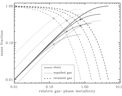
The simple model demonstrates that the gas-phase metallicity can be a relatively accurate predictor of a galaxy’s SF efficiency ($as/g_{i}$ or baryonic-to-stellar mass conversion factor) regardless of a wide range of outflow scenarios. If the retained gas is greater in mass than the expelled gas, the SF efficiency will be within 30% of the closed-box estimate derived from the metallicity regardless of the outflow factor. If there is significant expelled gas, using Eq. 8 to relate metallicity to the stellar mass fraction will result in an underestimate of $as/(as+g)$ and an overestimate of $as/g_{i}$. If there are continuing infalls and outflows (e.g. Dalcanton 2007; Erb 2008), the case is less clear because of the dependence on the metallicity of the infalling gas.

Figure 9 shows stellar mass-metallicity relation using gas-phase oxygen abundances estimated by Tremonti et al. (2004). This does not vary significantly with environment (Mouhcine, Baldry, & Bamford, 2007) suggesting that there is a fundamental relationship between the present-day stellar mass of a galaxy and its SF efficiency. Brooks et al. (2007) concluded from their modelling that “low star formation efficiencies … are primarily responsible for the lower metallicities of low-mass galaxies and the overall ${\cal M}$-$Z$ trend”.

Figure 9: The stellar mass-metallicity relation derived from the emission-line analysis by Tremonti et al. (2004). The squares represent the median while the lines represent the 16th and 84th percentiles in logarithmic mass bins. The dotted lines show the solar abundance value determined by Allende Prieto et al. (2001).

Note that the estimated metallicity can depend on the emission lines considered and the calibration (Kobulnicky & Kewley, 2004; Savaglio et al., 2005; Kewley & Ellison, 2008). However our consideration here is only that the measured ${\cal M}$-$Z$ relation implies an increase of average gas-phase metallicity with mass, and that the relation between metallicity and stellar mass is fairly tight.

4.2 Relating stellar mass to baryonic mass

The variation in SF efficiency implied by the ${\cal M}$-$Z$ relation allows one to estimate a baryonic MF. We assumed (i) the median measured oxygen abundances at a given stellar mass are representative of the average gas-phase metallicity in the inter-stellar medium, (ii) the yield is independent of galaxy mass and time, (iii) the closed-box model can be used to relate SF efficiency to oxygen abundance, and (iv) the SF efficiencies of the most massive galaxies are about 90%. Next, we defined a parametrisation to relate the total baryonic mass of a galaxy (${\cal M}_{b}$) to the SF efficiency:

$$\frac{as}{g_{i}}\equiv\frac{{\cal M}_{s}}{{\cal M}_{b}}=\frac{{\cal M}_{b}}{{\cal M}_{b}+{\cal M}_{0}}(e_{u}-e_{l})+e_{l}$$ (9)

where ${\cal M}_{0}$ is a characteristic mass, and $e_{u}$ and $e_{l}$ are upper and lower limits of the SF efficiency. Combining with Eq. 8, this parametrisation was fitted to the ${\cal M}_{s}$-$Z$ data (using O/H, Fig. 9, for $Z$). Figure 10 shows the SF efficiency versus $\log{\cal M}_{s}$ and $\log{\cal M}_{b}$ from the best-fit parametrisation ($\log{\cal M}_{o}=9.6$, $e_{u}=0.90$, $e_{l}=0.09$, $12+\log p=8.84$ where $p$ is the oxygen yield).

Figure 10: SF efficiency versus mass and the implied baryonic mass function. Upper panel: The model SF efficiency is defined as the mass in stars formed divided by the mass available to form stars over the life of a galaxy. This is plotted versus stellar mass (dotted line) and baryonic mass (solid line). The squares represent the O/H values of Fig. 9 converted using a monotonic relationship to efficiency determined from a closed-box model and plotted against stellar mass. Lower panel: The dotted line represents the GSMF from Fig. 6. The dashed line represents the implied baryonic mass function given the relationship between SF efficiency and stellar mass. The solid line represents a double Schechter fit to these data at ${\cal M}_{b}>10^{9}{\cal M}_{\odot}$ with faint-end slope $\alpha_{2}\simeq-1.9$. The dash-and-dotted line is this fit converted back to stellar mass. The arrows illustrate the relationship between baryonic and stellar mass in this simple model.

The implied relationship between stellar and baryonic mass was then used to compute the baryonic MF (from the GSMF or from the stellar masses of all the galaxies). This is shown by the dashed line in the lower panel of Fig. 10. The solid line is a fit to the MF at ${\cal M}_{b}>10^{8.5}{\cal M}_{\odot}$. The faint-end slope in this case is given by a steep $\alpha_{2}\simeq-1.9$ (parameters as per Eq. 3 are 10.675, 4.90, $-0.42$, 0.61, $-1.87$.)

The steep part of the baryonic MF is caused by the initially fairly steep GSMF at ${\cal M}_{s}<10^{9}{\cal M}_{\odot}$ coupled with an increase in gas-to-stellar (G-S) mass ratio from $\sim 1.5$ at $10^{9}{\cal M}_{\odot}$ to $\sim 4$ at $10^{8}{\cal M}_{\odot}$ to $\sim 8$ at $10^{7}{\cal M}_{\odot}$ (Fig. 10: dotted line in upper panel). Though the G-S mass ratios for low-mass galaxies are large they are in fact similar to those obtained directly from HI surveys. For example, the above values are similar to the ratios estimated by Kannappan (2004) for the low-mass end of the blue sequence.

In order to test the average G-S mass ratios implied by our parametrisation, we used stellar and atomic gas masses derived from the Westerbork HI Survey (Swaters & Balcells, 2002; Noordermeer et al., 2005) and the literature compilation of Garnett (2002). The stellar masses were estimated using the simple relations of Bell et al. (2003b) applied to the $B$ and $R$ photometry of Swaters & Balcells and the $B$ and $V$ photometry of Garnett, and using $\log({\cal M}_{s}/L_{B})=0.3$ for the early-type spirals of Noordermeer et al. We also matched the HI Parkes All-Sky Survey (HIPASS) catalogue (Meyer et al., 2004; Wong et al., 2006) to the NYU-VAGC catalogue. This resulted in 170 galaxies with one-and-only-one match within $0.25\degr$ and $\Delta zc<250{\rm\,km\,s}^{-1}$.

Figure 11 shows average G-S mass ratios in bins of stellar mass for these surveys; also shown is the relation derived from our parametrisation. The HIPASS mass ratios lie above this line, not surprisingly, because the HI selection misses galaxies with low G-S mass ratios. Thus these derived mass ratios should be regarded as upper limits. The G-S mass ratios derived from the optically-selected Westerbork survey are in good agreement, which lends support to our parametrisation of the SF efficiency. The Garnett compilation points to a flatter relation but this was using a significantly smaller, heterogeneously-selected sample.

Figure 11: Average atomic G-S mass ratios. The symbols represent G-S mass ratios from HI measurements with a 1.33 correction factor to account for Helium. The data from 4–25 galaxies were averaged for each point. The vertical error bars represent the standard errors; while the horizontal error bars represent the ranges of each sample. See text for further details. The dashed line represents the parametrisation of Eq. 9 assuming the closed-box model and that all the gas is atomic gas. The dash-and-dotted line represents the same parametrisation but assuming 70% of the gas is atomic gas. Note that gas-poor ellipticals are not considered in these samples, however, they are only a significant field population at $\ga 10^{11}{\cal M}_{\odot}$ and so their gas properties can be ignored in terms of computing the baryonic MF.

Various authors have found that the effective yield is lower in low mass galaxies (Garnett, 2002; Pilyugin et al., 2004; Tremonti et al., 2004) with an interpretation being that there is significant metal loss by metal-enriched outflows (Dalcanton, 2007). The effective yield is defined as

$$p_{\rm eff}=Z/\ln\left(\frac{as+g}{g}\right)$$ (10)

such that $p_{\rm eff}=p$ for the closed-box model, and $p_{\rm eff}<p$ with outflows. Our analysis uses SDSS-aperture metallicities and a closed-box model to predict average gas masses. This gives approximately correct global G-S mass ratios at least in comparison with the Westerbork samples (Fig. 11), which is consistent with the variation in SF efficiency with mass being the primary cause of the ${\cal M}_{s}$-$Z$ relation (see also Brooks et al. 2007; Ellison et al. 2008; Mouhcine et al. 2008; Tassis et al. 2008). This does not mean that there are no significant outflows, only that they may be a secondary cause of the ${\cal M}_{s}$-$Z$ relation.

The precise shape and steepness of the baryonic MF does depend on the detail of the G-S mass ratios and the dispersion in the relationship with stellar mass. However, our main aim is to illustrate the relationship between galaxy baryonic mass function and GSMF, and so we use the simple stellar-to-baryonic mass relation derived here. We also note that while the change in slope converting from the GSMF to the baryonic MF could be exaggerated, the GSMF slope may be underestimated and so the faint-end slope of the baryonic MF could be $\sim-1.9$ even accounting for a more complicated relation.

4.3 Comparison between galaxy and halo baryonic mass functions

The implied baryonic mass function (Fig. 10) can be considered to be the sum of stars and any gas involved with the cycle of SF, in and around each galaxy, as long as the relationship between ${\cal M}_{s}/{\cal M}_{b}$ and $Z$ is not strongly affected by outflows. Other estimates of the baryonic MF have been made by Bell et al. (2003a), Read & Trentham (2005) and Shankar et al. (2006). These include stars and atomic gas in galaxies, and molecular gas in the case of the first two estimates.

Figure 12 shows a comparison between the implied baryonic mass function and the diet Salpeter version from Bell et al. (2003a). There is a significant offset between them, which can be reconciled by (i) allowing for the number density and missing light corrections of § 3.2 and (ii) slightly lowering the masses of Bell et al. because the stellar M-L ratios appear on the high side (§ 2). This is partly because of using the diet Salpeter IMF compared to those of Kroupa or Chabrier (Appendix). After plausible corrections, the galaxy baryonic MFs are in good agreement. There is no clear evidence for a steep slope at ${\cal M}\la 10^{9.5}{\cal M}_{\odot}$ in the Bell et al. function, but given the large error bars, it is consistent with the steep slope we find. Neither Read & Trentham (2005) or Shankar et al. (2006) noted such a steep slope in the baryonic MF. Shankar et al.’s G-S mass ratios were based on a calibration of HI and stellar masses as a function $B$-band luminosity (from Salucci & Persic 1999). Their average G-S mass ratio is $\sim 1$ at ${\cal M}_{s}=10^{8}{\cal M}_{\odot}$, which is significantly lower than our estimate.

Figure 12: Comparison between galaxy and halo baryonic mass functions. The thick dotted line represents the MF determined by Bell et al. (2003a); with the thin dotted line representing masses reduced by 15%. Error bars are shown for the low-mass end. The thick solid line represents the MF from Fig. 10; with the thin line representing masses increased by 20% and number densities by 13% (cf. § 3.2). Halo MFs with masses multiplied by $\Omega_{b}/\Omega_{m}$ are shown by the dashed lines (Millennium Simulation; Sheth & Tormen 1999 using longer dashes), and by the dash-and-dotted line for the ‘galactic halo MF’ (Shankar et al., 2006).

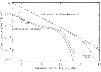
For comparison, halo MFs are shown in Fig. 12 assuming a constant fraction of mass in baryons in each halo ($\Omega_{b}/\Omega_{m}$). The long-dashed line was derived from the simulations of Sheth & Tormen (1999) while the dashed line was derived from the Millennium Simulation (Springel et al., 2005). The SF efficiency implied by the ${\cal M}_{s}$-$Z$ relation shows that the galaxy baryonic MF is approximately as steep, at ${\cal M}_{b}<10^{9.5}{\cal M}_{\odot}$, as the halo MF. The ‘galactic halo MF’ given by eq. 9 of Shankar et al. (2006) is also shown. This galactic halo MF, which includes halos and sub-halos hosting a galaxy but not group and cluster halos, is very similar in shape to the standard halo MF at ${\cal M}_{b}\la 10^{11}{\cal M}_{\odot}$. This is because the slopes of sub-halo MFs do not depend strongly on the mass of the main halo and have values similar to that of the halo MF (De Lucia et al., 2004; Reed et al., 2005).

To illustrate the implications of the form of the mass functions on galaxy formation efficiency, we computed the efficiency as a function of halo baryonic mass required to reproduce the galaxy MFs. This assumes a one-to-one and monotonic relationship between halo mass and galaxy mass. In detail this is described by Shankar et al. (2006), and earlier using galaxy luminosity by Marinoni & Hudson (2002) and Vale & Ostriker (2004). For the halo MF, we use the galactic halo MF with mass multiplied by $\Omega_{b}/\Omega_{m}$. Figure 13 shows the efficiency versus halo mass and the reconstructed galaxy MFs. The efficiency represented by the solid line can be regarded as the fraction of baryons that fall onto a galaxy and are available for forming stars; while the dashed line represents the fraction of baryons that have formed stars. These reproduce the galaxy baryonic MF and GSMF, respectively.

Figure 13: Idealised reconstruction of galaxy formation efficiency. The top panel shows the fraction of baryons falling onto a galaxy (solid line) and the fraction of baryons forming stars (dashed line). The lower panel shows the result of using the efficiency curves to go from the galactic halo baryonic MF (dash-and-dotted line) to the galaxy baryonic MF (solid line) and to the GSMF (dashed line). A standard halo baryonic MF that does not distinguish between galactic, group and cluster halos is shown by the dotted line. The arrows illustrate the relationships between the mass functions. They are not flat because the number density per logarithmic bin changes depending on the derivative of efficiency with respect to mass.

The figure demonstrates the implication that there is a levelling off of the baryonic-infall efficiency at low masses, while SF efficiency continues to fall, and shows a peak galaxy formation efficiency at $10^{11.1}{\cal M}_{\odot}$ ($10^{11.9}{\cal M}_{\odot}$ including CDM). Shankar et al. (2006) also looked at SF efficiency versus halo mass and demonstrated a similar result (their fig. 5) albeit with a flatter falloff at higher masses and a steeper falloff at lower masses related to the different GSMF utilised by them. The reduced efficiency above and below this scale are inherent in recent semi-analytical models of galaxy formation including SF and active galactic nuclei feedback (Bower et al., 2006; Cattaneo et al., 2006; Croton et al., 2006). The scale is related to a minimum in feedback effects (cf. fig. 8 of Dekel & Birnboim 2006).

5 Summary and conclusions

The field low-redshift GSMF has been generally measured down to $\sim 10^{8.5}{\cal M}_{\odot}$ (Fig. 1). This accounts for the majority of stellar mass in the universe. The SMD of the universe is in the range 5–7 per cent of the baryon density (conservatively 4–8 per cent, assuming $\Omega_{b}=0.045$). The sources of uncertainty are corrections for dust attenuation, underlying stellar M-L ratios, missing low-SB light, and normalisation of the GSMF.

We determined the field GSMF using the SDSS NYU-VAGC low-redshift galaxy sample. At masses below $\sim 10^{9}{\cal M}_{\odot}$, the shape of the GSMF computed using a standard $1/V_{\rm max}$ approach was affected by LSS variations. This was corrected for using number density as a function of redshift of a volume-limited sample of galaxies (Fig. 3). Analysis of the bivariate distribution of stellar mass versus SB indicated that the number densities should be regarded as lower limits at masses below $\sim 10^{8.5}{\cal M}_{\odot}$ (Fig. 4). Despite this incompleteness, there is clear evidence for an upturn in the GSMF (Fig. 6) with a faint-end slope $\alpha_{2}\simeq-1.6$ (Eq. 3). This represents the power-law slope over the range $\la 10^{8}$ to $\sim 10^{9}{\cal M}_{\odot}$. Steeper slopes are also plausible. Slopes of $\sim-2$ have been measured in clusters over the same mass range (Fig. 7). The processes shaping the GSMF in clusters will include stripping of gas and stars, while feedback processes may be more dominant in shaping the field GSMF.

At masses below $10^{10}{\cal M}_{\odot}$, blue-sequence (late-type) galaxies are the dominant field population (e.g. fig. 10 of Baldry et al. 2004). The gas-phase metallicity of these galaxies can be related to a SF efficiency that is defined as the total mass of stars formed divided by the available baryonic mass for forming stars. The closed-box formula can remain a good estimate of the SF efficiency even with moderate outflows (Fig. 8), excluding the case of metal-enriched outflows for gas-rich systems (Dalcanton, 2007).

Using a simple relationship between stellar mass and baryonic mass, based on the ${\cal M}_{s}$-$Z$ relation and the closed-box formula for $Z$ that neglects outflows, we converted the field GSMF to an implied baryonic mass function (Fig. 10). The resulting faint-end slope $\alpha_{2}\sim-1.9$ is similar to the halo MF. We note that this is only suggestive as it depends on the form of the conversion between ${\cal M}_{s}$ and ${\cal M}_{b}$ and the dispersion in this relationship (Fig. 11). The shape of the galaxy baryonic MF is consistent with the non-parametric MF of Bell et al. (2003a) (Fig. 12).

Taking the shape of the implied baryonic mass function at face value, we compared this with a simulated halo baryonic MF. Using a one-to-one relationship between halos and galaxies, these can be used to determine the galaxy formation efficiency (the fraction of baryons falling onto a galaxy) as a function of halo mass (Fig. 13). This illustrates how varying efficiency with mass can be used to obtain galaxy mass functions from the halo MF, or from a similarly-shaped sub-halo MF. The peak in the formation efficiency curve may correspond to a minimum in feedback efficiency.

There is no evidence yet of any cutoff in mass, below which baryons do not collapse into galaxies (cf. Dekel & Woo 2003). Rather we find the baryonic-infall efficiency levels off to $\sim 10$% rather than continuing to plummet with mass. It is possible that a cutoff mass scale, imprinted in the shape of the field galaxy baryonic MF, could be found by future deeper surveys. To robustly identify this scale requires: (i) wide-field deep imaging with reliable identification of galaxies down to at least $\mu_{r}\sim 25{\rm\,mag\,arcsec}^{2}$; (ii) spectroscopy of large samples down to $r\sim 20{\rm\,mag}$, or a similar effective depth in near-IR selection, in order to obtain accurate distances ($z\ga 0.01$) and metallicities for low-mass galaxies; (iii) wide-field HI surveys in order to estimate gas masses more directly. The prospect of such a measurement within the next decade is good with the advent of new wide-field optical instruments and survey-efficient radio telescopes.

Appendix A Mass-to-light ratios of stellar populations

Stellar M/L ratios of galaxies are generally based on evolutionary population synthesis with the basic ingredient being simple stellar populations (SSPs). This section outlines some issues related to M/L determination: definition, IMF, metallicity, age, bursts, dust, synthesis code. [See also Portinari et al. (2004); Kannappan & Gawiser (2007).]

The following are common assumptions for estimating stellar masses. The IMF is valid from 0.1 to 100 (or 120) ${\cal M}_{\odot}$. Substellar objects, $<0.1{\cal M}_{\odot}$, are not included; from the Chabrier (2003) IMF, these add up to 5–10% of the stellar mass. Stellar remnants (white dwarfs, neutron stars, black holes) are included; this is typically a 10–20% factor in the PEGASE models. Stellar mass is the remaining mass in stars and remnants as opposed to the integral of the SF rate, i.e, ${\cal M}=(1-R)\int{\rm SFR}$ where $R$ is the recycled fraction. This is the definition used here and is appropriate considering the analysis of § 4.

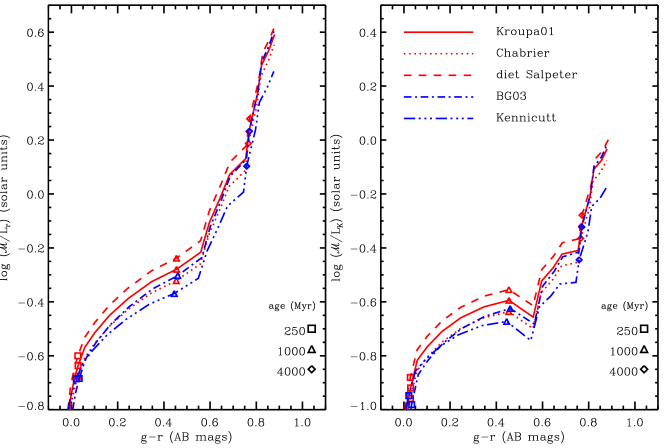
A significant factor is the choice of IMF. Figure 14 shows how M-L ratios in the $r$- and $K$-bands vary with IMF choice. The diet Salpeter has the highest masses considered here as it was calibrated to have maximum M-L ratios consistent with dynamical mass constraints (Bell & de Jong, 2001). Thus on the assumption of a universally-applicable IMF, this is the most-massive IMF at a given SSP colour that is valid. At the high-mass end of the IMF, steep slopes implying fewer high-mass stars are ruled out by measurements of cosmic luminosity densities (Baldry & Glazebrook, 2003). Thus reasonable M-L ratios are obtained with IMFs of Kroupa, Chabrier (0.91–0.93), diet Salpeter (1.07–1.11), Baldry & Glazebrook (0.90–1.04), and Kennicutt (0.74–0.88), where the ranges in parentheses are derived stellar masses relative to the Kroupa IMF at SSP colours evaluated over the range of 0.2–0.85 in $g-r$. [If the IMF varied with galaxy luminosity (Hoversten & Glazebrook, 2008), over time (Davé, 2008; van Dokkum, 2008) and/or in star bursts (Fardal et al., 2007), this would clearly complicate the determination of stellar masses.]

Figure 14: M-L ratios of simple stellar populations computed using PEGASE with ages from 100 Myr to 12 Gyr versus colour at solar metallicity. The left panel shows $r$-band M-L ratios while the right panel shows $K$-band M-L ratios. The tracks represent different IMFs (Kroupa, 2001; Chabrier, 2003; Bell & de Jong, 2001; Baldry & Glazebrook, 2003; Kennicutt, 1983). The upper-mass slopes of the IMFs are $\Gamma=1.3$, $1.3$, $1.35$, $1.15$, $1.5$, respectively (${\rm d}n/{\rm d}\log m\propto m^{-\Gamma}$). The low-mass slopes are reduced at $m<0.5$ or $<1{\cal M}_{\odot}$ except for the diet Salpeter, which uses a 0.7 correction factor.

A more significant consideration is the choice of prior (allowed SF histories, etc.) and population synthesis code. The following figures are provided to illuminate some of these considerations. Figure 15 shows M-L ratio versus colour for SSPs over a range of metallicities derived from PEGASE (Fioc & Rocca-Volmerange, 1997, 1999) and Bruzual & Charlot (2003) models. Figure 16 shows the effect of adding a 100-Myr burst contributing 5% of the stellar mass. Figure 17 shows a comparison between PEGASE and preliminary M-L ratios derived from BaSTI (M. Salaris, private communication; Pietrinferni et al. 2004). Figure 18 shows PEGASE models for SF histories with constant rate.

Figure 15: M-L ratios of simple stellar populations with ages from 100 Myr to 12 Gyr versus colour. The left panel shows $r$-band M-L ratios while the right panel shows $K$-band M-L ratios. The tracks represent different metallicities colour-coded according to the legend in the top-left of each panel. The arrows correspond to the effect of $A_{v}=1{\rm\,mag}$ of dust attenuation for an SMC screen law (thicker line) and a $\lambda^{-0.7}$ power law.

Figure 16: As per Fig. 15 except a ‘burst’ corresponding to an SSP of 100 Myr contributing 5% of the stellar mass has been added to each population. Since the SSPs are plotted from 100 Myr, the tracks start in the same position as Fig. 15.

Figure 17: As per Fig. 15 except comparing M-L ratios from BaSTI with PEGASE. The BaSTI models cover a larger metallicity range than implied by the legend with [Fe/H] from 0.4 to $-2.3$.

Figure 18: As per Fig. 15 except for constant-rate SF histories.

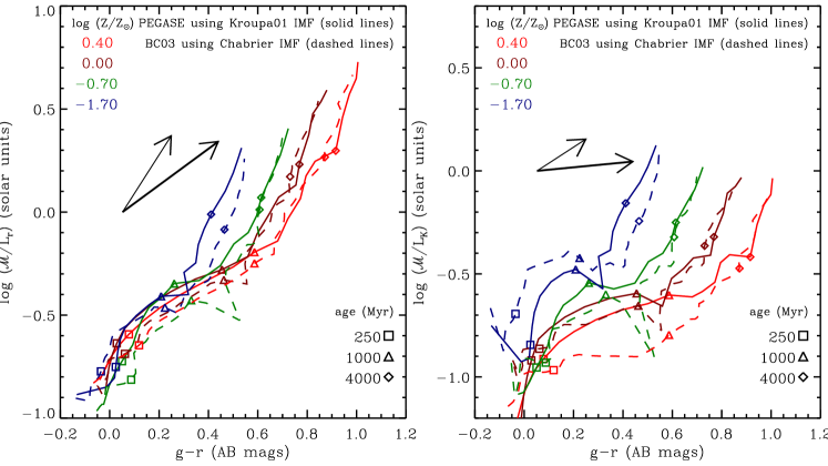
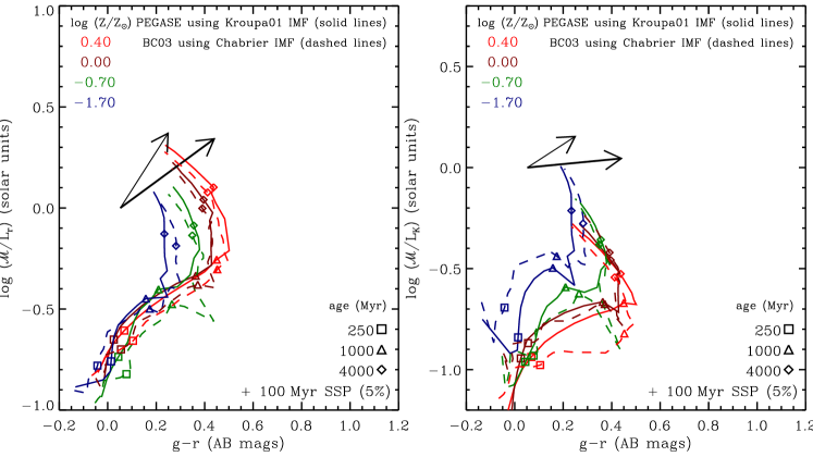
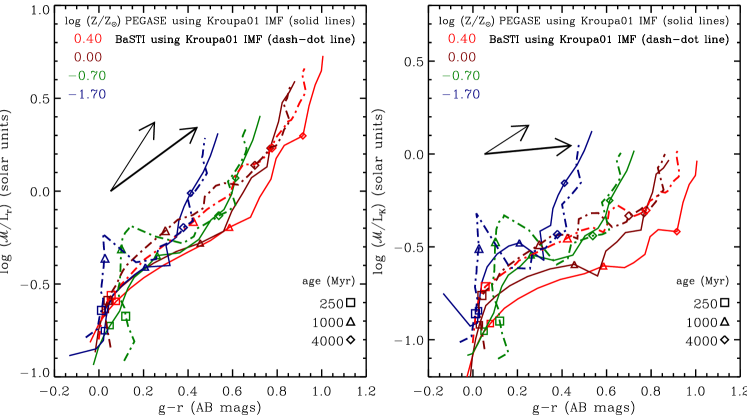
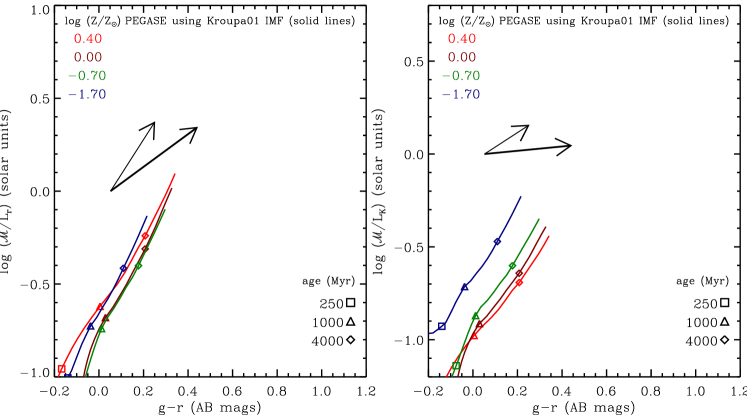
Last but not least, there is the complication of dust attenuation. The arrows in Figs. 15–18 show the effect of 1 magnitude of attenuation, at the $V$ band, on the colours and M-L ratios: both for a Small Magellanic Cloud (SMC) screen law (Pei, 1992) and a $\lambda^{-0.7}$ power law (Charlot & Fall, 2000). The latter law allows for a range of attenuation to different parts of a galaxy making it ‘greyer’ than a screen law.

An example of the importance of the prior and dust law is demonstrated by the fitting to the photometry of the NYU-VAGC sample (§ 3). Fitting only to photometry, as opposed to spectral features, has the advantage of being less sensitive to aperture bias but the disadvantage that colours are highly sensitive to dust attenuation. Various fits including different dust laws were tested (also fitting to $ugriz\,+\,JHK$). It was found that using a screen law significantly lowered the mass of luminous red galaxies (early types), which were fitted with significant dust attenuation, compared to assuming no dust. The lower masses occurred because younger-age models with dust reddening to reproduce the observed colours give lower M-L ratios than older-age models with no dust, i.e., the screen-law dust vector (change in M-L ratio as a function of colour) is shallower than the age vector for red galaxies (Fig. 15). Using a $\lambda^{-0.7}$ dust law did not lower the masses but early-type galaxies were still fitted with significant dust, which is not consistent with our general knowledge of these galaxies, unless the fitting was restricted to solar metallicity only. Comparable GSMFs were obtained either by allowing for varying dust attenuation and assuming solar metallicity or by allowing for a range of metallicities and assuming no dust. The former is more appropriate for the high-mass galaxies while the latter is more appropriate for low-mass, and low-metallicity, galaxies.

References

- Allende Prieto et al. (2001) Allende Prieto C., Lambert D. L., Asplund M., 2001, ApJ, 556, L63
- Baldry et al. (2006) Baldry I. K., Balogh M. L., Bower R. G., Glazebrook K., Nichol R. C., Bamford S. P., Budavari T., 2006, MNRAS, 373, 469
- Baldry & Glazebrook (2003) Baldry I. K., Glazebrook K., 2003, ApJ, 593, 258
- Baldry et al. (2004) Baldry I. K., Glazebrook K., Brinkmann J., Ivezić Ž., Lupton R. H., Nichol R. C., Szalay A. S., 2004, ApJ, 600, 681
- Balogh et al. (2001) Balogh M. L., Christlein D., Zabludoff A. I., Zaritsky D., 2001, ApJ, 557, 117
- Bell & de Jong (2001) Bell E. F., de Jong R. S., 2001, ApJ, 550, 212
- Bell et al. (2003a) Bell E. F., McIntosh D. H., Katz N., Weinberg M. D., 2003a, ApJ, 585, L117
- Bell et al. (2003b) —, 2003b, ApJS, 149, 289
- Belokurov et al. (2007) Belokurov V., et al., 2007, ApJ, 654, 897
- Binggeli et al. (1988) Binggeli B., Sandage A., Tammann G. A., 1988, ARA&A, 26, 509
- Blanton et al. (2005a) Blanton M. R., Lupton R. H., Schlegel D. J., Strauss M. A., Brinkmann J., Fukugita M., Loveday J., 2005a, ApJ, 631, 208
- Blanton et al. (2001) Blanton M. R., et al., 2001, AJ, 121, 2358
- Blanton et al. (2005b) —, 2005b, AJ, 129, 2562
- Bower et al. (2006) Bower R. G., Benson A. J., Malbon R., Helly J. C., Frenk C. S., Baugh C. M., Cole S., Lacey C. G., 2006, MNRAS, 370, 645
- Brooks et al. (2007) Brooks A. M., Governato F., Booth C. M., Willman B., Gardner J. P., Wadsley J., Stinson G., Quinn T., 2007, ApJ, 655, L17
- Bruzual & Charlot (1993) Bruzual G., Charlot S., 1993, ApJ, 405, 538
- Bruzual & Charlot (2003) —, 2003, MNRAS, 344, 1000
- Burles et al. (2001) Burles S., Nollett K. M., Turner M. S., 2001, ApJ, 552, L1
- Cattaneo et al. (2006) Cattaneo A., Dekel A., Devriendt J., Guiderdoni B., Blaizot J., 2006, MNRAS, 370, 1651
- Cen & Ostriker (1999) Cen R., Ostriker J. P., 1999, ApJ, 514, 1
- Chabrier (2003) Chabrier G., 2003, PASP, 115, 763
- Charlot & Fall (2000) Charlot S., Fall S. M., 2000, ApJ, 539, 718
- Cole et al. (1994) Cole S., Aragon-Salamanca A., Frenk C. S., Navarro J. F., Zepf S. E., 1994, MNRAS, 271, 781
- Cole et al. (2001) Cole S., et al., 2001, MNRAS, 326, 255
- Colless et al. (2001) Colless M., et al., 2001, MNRAS, 328, 1039
- Cross & Driver (2002) Cross N., Driver S. P., 2002, MNRAS, 329, 579
- Croton et al. (2006) Croton D. J., et al., 2006, MNRAS, 365, 11
- Dalcanton (2007) Dalcanton J. J., 2007, ApJ, 658, 941
- Davé (2008) Davé R., 2008, MNRAS, 385, 147
- De Lucia et al. (2004) De Lucia G., Kauffmann G., Springel V., White S. D. M., Lanzoni B., Stoehr F., Tormen G., Yoshida N., 2004, MNRAS, 348, 333
- Dekel & Birnboim (2006) Dekel A., Birnboim Y., 2006, MNRAS, 368, 2
- Dekel & Woo (2003) Dekel A., Woo J., 2003, MNRAS, 344, 1131
- Disney & Phillipps (1983) Disney M., Phillipps S., 1983, MNRAS, 205, 1253
- Disney (1976) Disney M. J., 1976, Nature, 263, 573
- Driver et al. (1994) Driver S. P., Phillipps S., Davies J. I., Morgan I., Disney M. J., 1994, MNRAS, 268, 393
- Driver et al. (2007) Driver S. P., Popescu C. C., Tuffs R. J., Liske J., Graham A. W., Allen P. D., de Propris R., 2007, MNRAS, 379, 1022
- Edmunds (1990) Edmunds M. G., 1990, MNRAS, 246, 678
- Efstathiou (1992) Efstathiou G., 1992, MNRAS, 256, 43P
- Efstathiou et al. (1988) Efstathiou G., Ellis R. S., Peterson B. A., 1988, MNRAS, 232, 431
- Ellison et al. (2008) Ellison S. L., Patton D. R., Simard L., McConnachie A. W., 2008, ApJ, 672, L107
- Elmegreen (2001) Elmegreen B. G., 2001, in Astron. Soc. Pacific Conf. Ser., Vol. 243, From Darkness to Light: Origin and Evolution of Young Stellar Clusters, Montmerle T., André P., eds., p. 255
- Erb (2008) Erb D. K., 2008, ApJ, 674, 151
- Fardal et al. (2007) Fardal M. A., Katz N., Weinberg D. H., Davé R., 2007, MNRAS, 379, 985
- Ferrara et al. (1999) Ferrara A., Bianchi S., Cimatti A., Giovanardi C., 1999, ApJS, 123, 437
- Fioc & Rocca-Volmerange (1997) Fioc M., Rocca-Volmerange B., 1997, A&A, 326, 950
- Fioc & Rocca-Volmerange (1999) —, 1999, PEGASE.2 documentation, arXiv:astro-ph/9912179
- Fukugita et al. (1998) Fukugita M., Hogan C. J., Peebles P. J. E., 1998, ApJ, 503, 518
- Gallazzi et al. (2008) Gallazzi A., Brinchmann J., Charlot S., White S. D. M., 2008, MNRAS, 383, 1439
- Gallazzi et al. (2005) Gallazzi A., Charlot S., Brinchmann J., White S. D. M., Tremonti C. A., 2005, MNRAS, 362, 41
- Garnett (2002) Garnett D. R., 2002, ApJ, 581, 1019
- Glazebrook et al. (2004) Glazebrook K., et al., 2004, Nature, 430, 181
- Harsono & de Propris (2007) Harsono D., de Propris R., 2007, MNRAS, 380, 1036
- Heavens et al. (2000) Heavens A. F., Jimenez R., Lahav O., 2000, MNRAS, 317, 965
- Hoversten & Glazebrook (2008) Hoversten E. A., Glazebrook K., 2008, ApJ, 675, 163
- Huang et al. (2003) Huang J.-S., Glazebrook K., Cowie L. L., Tinney C., 2003, ApJ, 584, 203
- Jansen et al. (2000) Jansen R. A., Franx M., Fabricant D., Caldwell N., 2000, ApJS, 126, 271
- Jarrett et al. (2000) Jarrett T. H., Chester T., Cutri R., Schneider S., Skrutskie M., Huchra J. P., 2000, AJ, 119, 2498
- Jenkins et al. (2007) Jenkins L. P., Hornschemeier A. E., Mobasher B., Alexander D. M., Bauer F. E., 2007, ApJ, 666, 846
- Kannappan (2004) Kannappan S. J., 2004, ApJ, 611, L89
- Kannappan & Gawiser (2007) Kannappan S. J., Gawiser E., 2007, ApJ, 657, L5
- Kauffmann et al. (1993) Kauffmann G., White S. D. M., Guiderdoni B., 1993, MNRAS, 264, 201
- Kauffmann et al. (2003) Kauffmann G., et al., 2003, MNRAS, 341, 33
- Kay et al. (2002) Kay S. T., Pearce F. R., Frenk C. S., Jenkins A., 2002, MNRAS, 330, 113
- Kennicutt (1983) Kennicutt R. C., 1983, ApJ, 272, 54
- Kewley & Ellison (2008) Kewley L. J., Ellison S. L., 2008, ApJ, in press (arXiv:0801.1849), 801
- Klypin et al. (1999) Klypin A., Kravtsov A. V., Valenzuela O., Prada F., 1999, ApJ, 522, 82
- Kobulnicky & Kewley (2004) Kobulnicky H. A., Kewley L. J., 2004, ApJ, 617, 240
- Kochanek et al. (2001) Kochanek C. S., et al., 2001, ApJ, 560, 566
- Kodama & Bower (2003) Kodama T., Bower R., 2003, MNRAS, 346, 1
- Kroupa (2001) Kroupa P., 2001, MNRAS, 322, 231
- Lacey & Silk (1991) Lacey C., Silk J., 1991, ApJ, 381, 14
- Loveday (1997) Loveday J., 1997, ApJ, 489, 29
- Loveday et al. (1992) Loveday J., Peterson B. A., Efstathiou G., Maddox S. J., 1992, ApJ, 390, 338
- Maller & Bullock (2004) Maller A. H., Bullock J. S., 2004, MNRAS, 355, 694
- Marinoni & Hudson (2002) Marinoni C., Hudson M. J., 2002, ApJ, 569, 101
- Martin et al. (2006) Martin N. F., Ibata R. A., Irwin M. J., Chapman S., Lewis G. F., Ferguson A. M. N., Tanvir N., McConnachie A. W., 2006, MNRAS, 371, 1983
- Marzke et al. (1998) Marzke R. O., da Costa L. N., Pellegrini P. S., Willmer C. N. A., Geller M. J., 1998, ApJ, 503, 617
- Meyer et al. (2004) Meyer M. J., et al., 2004, MNRAS, 350, 1195
- Moore et al. (1999) Moore B., Ghigna S., Governato F., Lake G., Quinn T., Stadel J., Tozzi P., 1999, ApJ, 524, L19
- Mouhcine et al. (2007) Mouhcine M., Baldry I. K., Bamford S. P., 2007, MNRAS, 382, 801
- Mouhcine et al. (2008) Mouhcine M., Gibson B. K., Renda A., Kawata D., 2008, A&A, in press (arXiv:0801.2476)
- Nagamine et al. (2006) Nagamine K., Ostriker J. P., Fukugita M., Cen R., 2006, ApJ, 653, 881
- Noordermeer et al. (2005) Noordermeer E., van der Hulst J. M., Sancisi R., Swaters R. A., van Albada T. S., 2005, A&A, 442, 137
- Norberg et al. (2002) Norberg P., et al., 2002, MNRAS, 336, 907
- Panter et al. (2004) Panter B., Heavens A. F., Jimenez R., 2004, MNRAS, 355, 764
- Panter et al. (2007) Panter B., Jimenez R., Heavens A. F., Charlot S., 2007, MNRAS, 378, 1550
- Pei (1992) Pei Y. C., 1992, ApJ, 395, 130
- Pietrinferni et al. (2004) Pietrinferni A., Cassisi S., Salaris M., Castelli F., 2004, ApJ, 612, 168
- Pilyugin et al. (2004) Pilyugin L. S., Vílchez J. M., Contini T., 2004, A&A, 425, 849
- Popesso et al. (2006) Popesso P., Biviano A., Böhringer H., Romaniello M., 2006, A&A, 445, 29
- Popesso et al. (2005) Popesso P., Böhringer H., Romaniello M., Voges W., 2005, A&A, 433, 415
- Portinari et al. (2004) Portinari L., Sommer-Larsen J., Tantalo R., 2004, MNRAS, 347, 691
- Read & Trentham (2005) Read J. I., Trentham N., 2005, R. Soc. Lond. Philos. Trans. Series A, 363, 2693
- Reed et al. (2005) Reed D., Governato F., Quinn T., Gardner J., Stadel J., Lake G., 2005, MNRAS, 359, 1537
- Salucci & Persic (1999) Salucci P., Persic M., 1999, MNRAS, 309, 923
- Savaglio et al. (2005) Savaglio S., et al., 2005, ApJ, 635, 260
- Schechter (1976) Schechter P., 1976, ApJ, 203, 297
- Shankar et al. (2006) Shankar F., Lapi A., Salucci P., De Zotti G., Danese L., 2006, ApJ, 643, 14
- Sheth & Tormen (1999) Sheth R. K., Tormen G., 1999, MNRAS, 308, 119
- Somerville (2002) Somerville R. S., 2002, ApJ, 572, L23
- Spergel et al. (2007) Spergel D. N., et al., 2007, ApJS, 170, 377
- Springel et al. (2005) Springel V., et al., 2005, Nature, 435, 629
- Stoughton et al. (2002) Stoughton C., et al., 2002, AJ, 123, 485
- Swaters & Balcells (2002) Swaters R. A., Balcells M., 2002, A&A, 390, 863
- Swaters et al. (2002) Swaters R. A., van Albada T. S., van der Hulst J. M., Sancisi R., 2002, A&A, 390, 829
- Tassis et al. (2008) Tassis K., Kravtsov A. V., Gnedin N. Y., 2008, ApJ, 672, 888
- Tinsley (1980) Tinsley B. M., 1980, Fundamentals of Cosmic Physics, 5, 287
- Tinsley & Gunn (1976) Tinsley B. M., Gunn J. E., 1976, ApJ, 203, 52
- Tremonti et al. (2004) Tremonti C. A., et al., 2004, ApJ, 613, 898
- Tuffs et al. (2004) Tuffs R. J., Popescu C. C., Völk H. J., Kylafis N. D., Dopita M. A., 2004, A&A, 419, 821
- Vale & Ostriker (2004) Vale A., Ostriker J. P., 2004, MNRAS, 353, 189
- van Dokkum (2008) van Dokkum P. G., 2008, ApJ, 674, 29
- White & Rees (1978) White S. D. M., Rees M. J., 1978, MNRAS, 183, 341
- Willick et al. (1997) Willick J. A., Strauss M. A., Dekel A., Kolatt T., 1997, ApJ, 486, 629
- Wong et al. (2006) Wong O. I., et al., 2006, MNRAS, 371, 1855
- York et al. (2000) York D. G., et al., 2000, AJ, 120, 1579
- Zucca et al. (1997) Zucca E., et al., 1997, A&A, 326, 477