Water at an electrochemical interface - a simulation study

Abstract

The results of molecular dynamics simulations of the properties of water in an aqueous ionic solution close to an interface with a model metallic electrode are described. In the simulations the electrode behaves as an ideally polarizable hydrophilic metal, supporting image charge interactions with charged species, and it is maintained at a constant electrical potential with respect to the solution so that the model is a textbook representation of an electrochemical interface through which no current is passing. We show how water is strongly attracted to and ordered at the electrode surface. This ordering is different to the structure that might be imagined from continuum models of electrode interfaces. Further, this ordering significantly affects the probability of ions reaching the surface. We describe the concomitant motion and configurations of the water and ions as functions of the electrode potential, and we analyze the length scales over which ionic atmospheres fluctuate. The statistics of these fluctuations depend upon surface structure and ionic strength. The fluctuations are large, sufficiently so that the mean ionic atmosphere is a poor descriptor of the aqueous environment near a metal surface. The importance of this finding for a description of electrochemical reactions is examined by calculating, directly from the simulation, Marcus free energy profiles for transfer of charge between the electrode and a redox species in the solution and comparing the results with the predictions of continuum theories. Significant departures from the electrochemical textbook descriptions of the phenomenon are found and their physical origins are characterized from the atomistic perspective of the simulations.

I Introduction

The altered solvation, dielectric and dynamical properties of water molecules close to electrode surfaces have an important influence on electrochemical reactions. There have been numerous simulation studies of aqueous solutions close to charged solid surfaces which have cast light on the ordering of water molecules by the solid surface and begun to make the connection between the layers with altered dielectric characteristics invoked in continuum models of the electrode capacitance and the ordered molecular films which are known from surface science. References neurock contain an excellent summary of work to date, and neurock1 ; spohr a more longstanding review. To complete the link between molecular behaviour and electrochemical observations we need a realistic representation of the electrochemical interface and a direct way of calculating the electrochemical observable, namely the dependence of the rate of the electrochemical electron transfer on the potential applied to the electrode bockris .

Figure 1: Schematic illustration of the Marcus construction for understanding the electrochemical oxidation of some species R= M⁺ to O=M²⁺ with transfer of the charge ($\delta q$) to an electrode maintained at a potential $V$. The quantities $\Delta A$, $\lambda$ and $\lambda^{\prime}$ are the reaction free-energy and reorganization energies for oxidation and reduction, respectively

What is required to achieve the second of these objectives is suggested by the Marcus theory of electron transfer marcus1 ; marcus2 . In a Marcus description of the oxidation of some solution species R to an oxidised species O by transfer of an electron to an electrode maintained at some potential $V$ with respect to the solution we construct curves, as illustrated schematically in figure 1, which describe how the free energies of O and R depend upon some reaction coordinate, which is envisaged as reflecting the influence of fluctuating solvent degrees of freedom. The Marcus expression for the rate of electron transfer can be calculated from the probability that the system will access the configuration where the two curves cross. Note that the free energy curve for O includes the potential energy of the electron on the electrode ($eV$), so that the position and height of the crossing point depend on the electrode potential. The two curves are coupled by a term ($\gamma$) which reflects the tunneling of the electron between the redox centre and the electrode, and this is expected to depend exponentially on its distance from the electrode surface. We should, therefore, be thinking about the dependence of the Marcus curves on the proximity to the electrode surface, to which two factors contribute. Firstly, the difference between the direct interactions of the O and R species with the charged surface itself will produce a differential shift on them, and therefore affect the crossing point. Secondly, if the redox species is close to the electrode, the competing interactions of the water molecules in its coordination shell with the surface and the solute itself may result in a change in the character of the fluctuations of the reaction coordinate. Both of these factors may be affected by the potential applied to the electrode. The Marcus curves contain the information which is required to calculate the electron transfer rate for a redox ion at a given distance from the electrode surface, but to complete the calculation of the rate we also need to know the probability of the reactant reaching this position, and this too will be affected by the potential exerted by the electrode and its influence on the solvating properties of the water molecules.

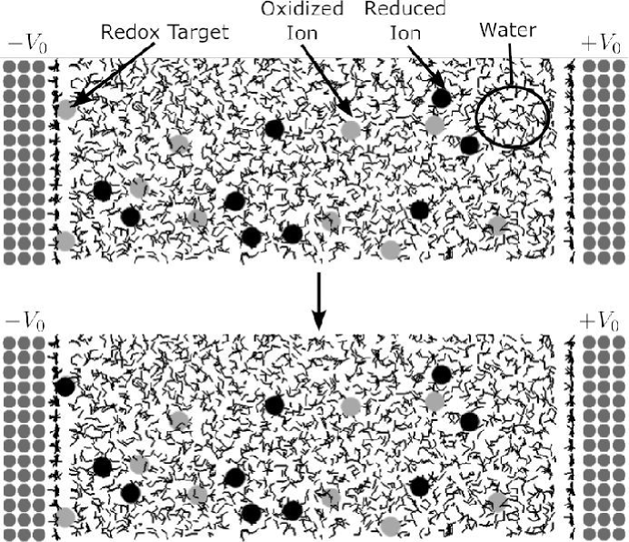
Figure 2: Schematic depiction of electron transfer

Blumberger, Sprik and co-workers sprik1 ; sprik2 have demonstrated how the Marcus curves can be calculated for a homogeneous electron transfer reaction within an ab initio molecular dynamics scheme. Following Warshel warshel they emphasize the advantages for computation of choosing the “vertical energy-gap” as the reaction coordinate. The vertical energy gap for oxidation is calculated for a single configuration in a simulation by switching the identity (and all associated interaction parameters) of a redox species initially in its reduced form R to its oxidised form without allowing any changes in the nuclear coordinates (hence a “vertical” transition in the Franck-Condon sense) and evaluating the energy difference between the final and initial states. The Marcus curves for the oxidised and reduced species may then be estimated from the probability distributions of the vertical energy gaps obtained by repeatedly sampling through the course of an molecular dynamics (MD) simulation and assuming this distribution is Gaussian. The Gaussian assumption is required by this method because regions of the distribution pertinent to the charge transfer reaction are not generally accessed in a straightforward simulation. In the calculations reported here, the Gaussian approximation is tested and shown to be accurate. More generally, the Gaussian approximation has been tested and found to be accurate chandler1 ; chandler2 provided proper account is taken of molecular boundary conditions chandler3

Use of this scheme to study the electrochemical electron transfer process in a simulation is illustrated in figure 2. An aqueous solution is contained between two crystalline arrays of atoms which comprise the (metallic) electrodes, these are maintained at a definite electrical potential. The solution contains the redox species in its reduced and oxidised forms and, periodically during the simulation, an ion (the “redox target”) is selected and its redox state is switched and the energy difference between final and initial states is evaluated. By selecting ions at different distances from the electrodes and by examining how the vertical energy gaps depend on the applied potential we can build up the necessary information to study how the nature of the water at the electrode surface affects the electrochemical electron transfer rate via the Marcus construction.

In order to make contact with experimental studies the calculation needs to be done with as realistic representation of the constant-potential electrode and interfacial water as can be managed. Ideally, it would be done within an ab initio MD scheme, as this would enable the difficult-to-characterise interactions between the solution and the electrode to be modelled without the introduction of interaction potentials neurock ; halley ; voth . However, the time and length scales involved in the relaxation of the solution in the vicinity of the electrodes (which we will characterise below) are far too long to allow a full self-consistent description of the screening of the electrode potential within an ab initio scheme halley-acs . Recently we introduced a way of incorporating some of the essential physical effects necessary for a realistic description of the interfacial charge-transfer process into a simulation which uses interaction potentials and therefore enables simulations of much larger time and length scales than is possible ab initio reed1 . In particular, model metallic electrodes maintained at a constant electrical potential may be introduced into such a simulation, following a technique introduced by Siepmann and Sprik siepmann . Because the electrodes behave as ideally polarizable metals they support image-charge interactions between charged species and the electrode; these, as we shall see, have an important influence on the electron transfer process. Because the electrodes are maintained at a constant potential when the charge of the redox species is changed to sample the vertical energy gap, that charge is transferred in full to the electrodes, so that the source of the dependence of the electron-transfer rate on the electrode potential is included in the calculation. The electrode potential and the potential felt by the molecules and ions in the solution region are calculated self-consistently. Calculations using these methods have already been performed to examine the Marcus curves in simulations of redox active molten salts reed2 .

We begin with a brief description of the methods and interaction potentials used to simulate pure water and aqueous solutions of LiCl and the Ru²⁺/Ru³⁺ couple confined between model platinum electrodes. We then examine the structure and dynamical properties of the electrode-adsorbed water and the way they are affected by the application of a potential to the electrode. In sections III and IV we consider the consequences of this adsorbed water for the approach of ions to the electrode surface and the effect of the adsorbed water and the ionic atmosphere for the electrical potential in the vicinity of the electrode. In classical models of electrochemical charge transfer this potential is invoked to represent the dependence of the energies of the oxidised and reduced species on the proximity to the electrode. We then present preliminary results for the Marcus curves for the Ru²⁺/Ru³⁺ system and discuss the physical factors which determine their dependence on the applied potential and the proximity to the electrode.

II Scope of the model.

The electrochemical interface is affected by many phenomena and a comprehensive representation of all of them within a single simulation is beyond current capabilities. Our focus here is on the solution side of the interface, on the properties of the water molecules at the interface and their influence on the electrical potential. As such we will present a significantly simplified model of the electrode itself in which we ignore the motion of the electrode atoms and therefore neglect effects like the restructuring of the electrode surface under chemical or electrical influences kolb . Furthermore the representation of the electrode as a metal is a simplified one, designed to capture the correct macroscopic response to an electrical potential appropriate to a metal rather than to deal with a correct microscopic description of surface electronic states etc.

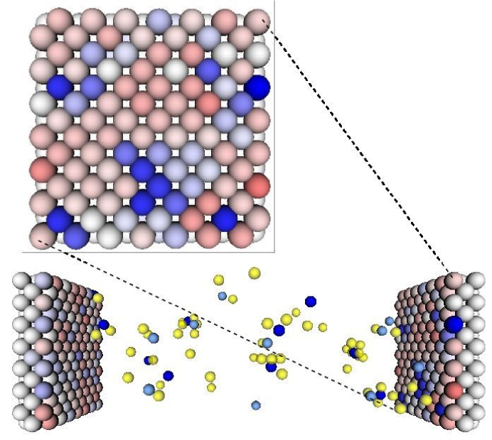
Figure 3: Snapshot of the distribution of charge on the polarizable model electrode. Electrode atoms are shaded according to their partial charge, with blue shading corresponding to positive charge and red shading corresponding to negative charge. In this rendering, the darkest shade of blue corresponds to a partial charge of $0.1e$, and the darkest shade of red to a partial charge of $-0.1e$. In the solvent region the yellow spheres represent $\mathrm{Cl^{-}}$ ions, and the light blue and dark blue spheres represent $\mathrm{Ru^{2+}}$ and $\mathrm{Ru^{3+}}$ respectively. Water molecules have been omitted for clarity.

As illustrated in figures 2 and 3, the electrodes each consist of three layers of atoms arranged in an fcc lattice with the 100 face exposed to the solution; the lattice parameter is appropriate to Pt. Following Siepmann and Sprik siepmann each electrode atom $i$ carries a Gaussian charge distribution of fixed width but variable amplitude ($q_{i}$). These charges are coulombically coupled to all other charges in the system. They are treated as additional dynamical degrees of freedom whose values are adjusted at each timestep in the molecular dynamic procedure in order to variationally minimise an appropriate energy functional. The energy functional is chosen siepmann so that at its minimum the electrical potential on every electrode atom is the same (as approriate to a metal) and equal to some pre-set value $V_{0}$. The use of a variational principle allows forces and response behaviour to be calculated straightforwardly via an application of the Hellmann-Feynman Theorem, as used to good effect in ab initio MD simulations. The methodology for the simulation of the electrodes is described in great detail in ref reed1 , where it is shown that the electrodes become polarised in the presence of a charge in the solution region in a way which corresponds to the classical image-charge response. We illustrate this response in figure 3 where the charge induced on the electrode atoms by the instantaneous configuration of the charges in solution is shown by colour-coding the electrode atoms. The bright blue region, for example, is caused by the presence of an anion within the first molecular layer of the solution close to this position. Furthermore, if the charge on one of the ions in solution is changed, the charge difference is fully transferred to the electrodes to maintain charge neutrality with a constant electrode potential reed2 : it is this feature which enables us to calculate Marcus curves for electrochemical charge transfer.

To describe the interactions between water molecules we use the SPC/E potential SPCE , which is known to give a dielectric constant for water close to the experimental value. The interactions of water molecules with a metallic electrode are complex, and cannot be modelled accurately with a simple two-body potential; since the behaviour of water at the interface is the central purpose of our study we were concerned to represent this interaction as carefully as is possible through the introduction of a potential. Experiment thiel and ab-initio studies holloway have shown that water molecules interact with a crystalline platinum surface by adsorbing on top sites and orienting their dipole along the plane of the electrode. In their study of water at an STM tip, Siepmann and Sprik siepmann parameterized a two- and three-body potential to describe the adsorption of water molecules on a platinum surface; their potentials are particularly appropriate for our study since they do not include the consequences of image interactions, which are dealt with through the polarizable electrode model as in our simulations. We have used these potentials exactly as described in their paper.

We have not attempted the same level of realism with the interactions between the ions and the electrode surface. Experimental studies show that anions interact quite strongly with transition metal surfaces to the extent that complete surface coverage of ordered layers of Cl^- is observed on positively charged single-crystal electrodes above about 0.5 V from molar solutions magnussen . Guymon et al have shown how suitable potentials to describe these strong interactions could be obtained from ab initio calculations guymon . However, adsorption of this strength would present a significant problem for our simulations since it would mean that the solution region would be strongly depleted in Cl^- ions. To represent the interface under these conditions we would need to equilibrate our system in the presence of a reservoir of electrolyte; furthermore equilibrating this system would be very slow, as we shall see. We have, therefore, for the present study introduced only weakly attractive interaction potentials between the ions and the electrode surface – we use exponential-6 potentials to represent the short-range interactions with the parameters chosen as if the atoms of the metallic walls were themselves Cl^- ions. These potentials are too weakly attractive, compared to the water-electrode interactions, to lead to the kind of anion adsorption phenomena seen in the experimental studies of Cl^--containing electrolytes. We note that fluoride ions are not thought to form adsorbed layers magnussen and so the picture of the interface we present may be more representative of a fluoride than a chloride-containing solution.

The interactions between the other species present in solution were modelled with pair potentials; this too reflects a compromise in the realism of the calculations as it is known that polarisation effects have a significant influence on the way that ions interact and coordinate water polarizable-ion-water . The water-ion interactions were modelled with a Lennard-Jones potential acting between the ion and the oxygen center of the water molecule. The parameters used in these interactions were adapted from Lynden-Bell bell1 . The ruthenium ion - water interactions were parameterized with a purely repulsive potential,

$$U_{\mathrm{Ru},\mathrm{O}}=A/|\textbf{r}_{\mathrm{Ru}}-\textbf{r}_{\mathrm{O}}|^{9},$$ (1)

with the parameter ($A=49977.9k\mathrm{Jmol^{-1}\AA^{9}}$ for both Ru²⁺ and Ru³⁺) chosen so that the first peaks of the ion-water radial distribution agreed with those obtained in an ab initio MD study sprik_ru . The ions interact with each other with exponential-6 potentials with the Ru-Cl potentials taken from lanthanides of corresponding ionic size morgan ; hutchinson .

III Pure water results

Figure 4: The Poisson potential across the model electrochemical cell for pure water. The oscillations near the electrodes result from ordering of the solvent in the vicinity of the electrode.

We begin by showing, in figure 4, results obtained for the profiles across the cell of the mean electrical (or “Poisson”) potential, $\Psi$, in pure water. This is obtained by integrating Poisson’s equation,

$$\nabla^{2}\Psi=-\frac{\rho}{\varepsilon_{0}}\;,$$ (2)

with the mean charge density, $\rho$, calculated from the simulation for different values of the applied electrode potential, $V_{0}$, as the source term ($\varepsilon_{0}$ is the permittivity of free space). The Poisson potential is the potential used in describing the potential at the electrochemical interface in classical theories and is therefore an important point of contact between our calculations and textbook descriptions of the electrochemical interface bockris ; kornyshev . The potential is constant on the interior of the electrodes and equal to the applied potential. It then drops rapidly and oscillates across an interfacial region about 12 Å wide, for reasons we will discuss in detail below, before settling down to acquire the constant slope appropriate to the behaviour of the potential in a bulk dielectric subject to an external potential. Notice that, other than at $V_{0}=0$, the potential drops across the two interfaces are not symmetrical because of the different microscopic arrangements of the water molecules at positively and negatively charged surfaces.

We can calculate a value for the dielectric constant of water from the behaviour of the potential across the bulk region. By integrating the mean charge in the region of the cell to the left of 20 Å  we can obtain a value for the charge, Q, on one plate of a virtual parallel plate capacitor placed at this position; the region to the right of 61.5 Å  has an equal and opposite charge and can be regarded as the other plate. The potential drop between the two plates is $\Delta\Psi$ and we can obtain values for the capacitance $C$ from $Q=C\Delta\Psi$ for the different applied potentials. This calculated capacitance $C$ can be compared with theoretical expression for capacitance of parallel plates filed with a medium of dielectric constant $\varepsilon$,

$$C=\varepsilon\varepsilon_{0}A/d,$$ (3)

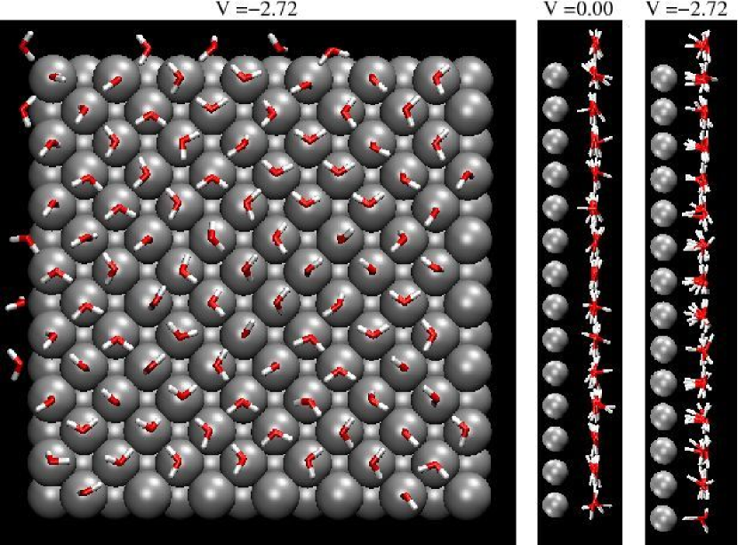
Figure 5: A snapshot of the adsorbed water layer, and their profiles at different values of the applied potential $V_{0}$. The orientation of adsorbed water molecules is noticeably altered by the change in electrode potential.

where $A$ is the cross-sectional area of the cell and $d$ the distance between the plates. The calculation shows that the dielectric constant for SPC/E water depends on the applied electrode potential. Specifically, when the electrode potential has the values $V_{0}=0.27$ V, $V_{0}=1.36$ V, and $V_{0}=2.72$ V, the dielectric constant for the bulk water is $\epsilon=75.07$, $\epsilon=61.50$, and $\epsilon=57.30$ respectively. The low voltage result is in reasonable agreement with direct simulation studies (68$\pm$5.8 steinhauser ), which is good confirmation that the potential and the response of the water molecules to it are correct (see also reference reed1 ). The reduction in the apparent dielectric constant at higher voltages is consistent with a saturation effect berkowitz , note that the potential difference of $\Delta\Psi\simeq$ 1.1 V, obtained with $V_{0}$=2.72 V, across our virtual capacitor of width 41.5 Å  is equivalent to an electric field of $\simeq 2.6\times 10^{8}$ Vm^-1.

The rapid oscillation of the potential close to the interfaces is due to the strong adsorption of a layer of water molecules at the electrode surfaces. This is illustrated in figure 5. The oxygen atoms of the water molecules form a commensurate layer on the top-sites of the underlying 100 fcc surface. With zero applied potential the water molecules lie with at least one O-H bond in the plane of the interface with the H-atom pointing towards a neighbouring oxygen and form ordered domains which reorient on a long timescale. Although the predominant orientation is in-plane, at zero applied potential there is a net orientation of the negative ends of the molecular dipoles towards the surface and this induces a small positive charge on the electrode atoms berkowitz .

When the potential is applied to the cell, the water molecules in the first layer partially reorient in the interfacial field. This is illustrated in the right-most panel of figure 5 where one of the OH bonds of the water molecules at the negatively charged electrode may point towards the electrode surface (note that this potential is very large for aqueous electrochemistry). The consequences of this for the Poisson potential can be see by reference to the right-hand interface in figure 4. Whereas at $V_{0}=0$ the potential initially drops on moving into the electrolyte, consistent with the negatively charged oxide ions being closest to the surface, at the applied potential of $V_{0}=-2.72$ V, the potential now rises showing an excess of positive charge lying close to the surface.

Figure 6: The distribution of $\cos(\theta)$ where $\theta$ is the angle between a water’s O-H bond vector and the vector normal to the electrode surface (pointing into the bulk). The left-hand panel is the distribution taken over the first two solvent layers adjacent to the positive electrode, and the right-hand one the distribution taken over the first two solvent layers adjacent to the negative electrode.

We can track these changes by showing the probability distributions of the orientation of O-H bonds in the first and second layers of water molecules as the applied potential is changed. We compute the probability distribution function $P[\cos(\theta)]$, where $\theta$ is the angle between an OH bond vector (the vector extending from the oxygen centre of a water molecule to the centre of one of the associated hydrogen atoms) and the the outward normal vector to the electrode surface. Fig 6 shows the distribution $P[\cos(\theta)]$ for different values of applied potential for the two electrodes. The left-hand panel of figure 6 shows the results at the positively charged electrode and the right-hand panel at the negatively charged one. At all values of the potential, the probability distribution is peaked around $\cos(\theta)=0$, corresponding to configurations for which the OH vector of a water molecule is aligned with the plane of the electrode surface. At zero applied potential the distribution $P[\cos(\theta)]$ for the adsorbed molecules is the same for the two electrodes, but even at $V_{0}=0$ there is an excess of outward (negative $cos(\theta)$) over inward pointing OH bonds, which give rise to the potential drop between the electrode and solution noted above. At different values of applied potential the distribution of OH vectors is changed significantly. At the positive electrode (left panel of Fig. 6) the main effect of the electrode potential is to deplete the population of OH bonds pointing into the electrode ($\cos(\theta)<0$). At the negative electrode (right panel of Fig. 6) however, at increased electrode potential there emerges a large population of OH vectors which point into the electrode. This change in orientational structure at the negative electrode is yet another demonstration of the asymmetry between the solvent structure at the positive and negative electrode.

Figure 7: The left-hand panel shows the distribution of the charges on the atoms which make up the innermost layer of the negative electrode. The changes in the orientations of the water molecules are accompanied by the development of a bimodal distribution of wall charges. The right-hand panel contrasts the O-H bond $\cos(\theta)$ distributions obtained in constant potential (figure 6) and constant charge simulations; the former are shown by lines and the latter by symbols.

The orientation of the adsorbed water molecules influences the charge induced on the electrode atoms on which they sit. Figure 7 shows the distributions of the charges induced on the atoms which make up the outermost layer of atoms on the negatively charged electrode. At zero applied potential the average charge is small and positive, for the reasons discussed above, but there is a significant number of negatively charged atoms which are associated with an adsorbed water molecule with an inward-pointing O-H bond. As the electrode potential becomes increasingly negative, so does the mean charge, but the bimodal character of the distribution becomes even more pronounced as more water molecules flip an O-H bond towards the electrode.

One question which arises from these results is the extent to which they are influenced by the inclusion of image charge interactions in the potential model. A way of addressing this question is to carry out constant charge simulations in which the values of the charges on the electrode atoms are fixed at the values of the average charges on the first, second and third layers of the electrode atoms obtained in constant potential runs with an electrode potential $V_{0}$. These static charge distributions generate similar electrode potentials to the $V_{0}$ values used in the constant potential runs used to generate them. It can be seen, from the right-hand panel of figure 7, that the dynamical nature of the charges in the constant potential simulations has only a small effect on the mean orientational distributions of the water molecules in the adsorbed layer and none on the second layer. However, as illustrated in figure 7 left-hand panel, there is a local response of the electrode in the constant potential simulations and this is responsible for the emergence of a significant population of electrode-pointing OH bonds in the directly adsorbed molecules; it is not observed in the simulations run at constant charge. The relatively small effect of the image charges on average interfacial structure parallels the findings in the molten salt simulations reed1 .

Figure 8: The variation of the potential drop across the double layer, $\Delta\Psi$, with electrode charge density, $q_{m}$, for water and LiCl(aq) for the positive and negative electrodes. The lines, whose slopes represent the differential capacitance of the positive and negative double layers are least squares fits to the water data.

The layering of solvent and the molecular orientations within the layers adjacent to the electrode affect the capacitance of the electrode, which can be measured experimentally. The capacitance of the first two layers of solvent can be calculated through the differential capacitance, $C=(\partial q_{m}/\partial\Delta\Psi)$, where $q_{m}$ is the charge density on the electrode and $\Delta\Psi$ is the potential drop across the first two layers of water. Figure 8 shows the dependence of $\Delta\Psi$ on $q_{m}$ for several values of the applied potential. The plot reveals that the potential of zero charge (pzc) for our simulated system is at -0.8 V. Comparing this quantity with experiment is not straightforward, since in the experimental measurements the potential is quoted with respect to a reference electrode whereas we can access directly the potential difference between the interior of the electrode and the solution. The experimental value with respect to a standard hydrogen electrode is +0.41 V bockris . The capacitance for electrode potentials which are on the positive side of the potential of zero charge ($C=8.39\mu\mathrm{F/cm^{2}}$) is larger than for negative potentials, $C=5.20\mu\mathrm{F/cm^{2}}$. Both values are considerably lower than predicted through experimental data which measures the the double layer capacitance in the range of $C=20-50\mu\mathrm{F/cm^{2}}$ kolb ; parsons close to the pzc. The substantial difference between our calculated value and experiment is not surprising as our model does not include a realistic description of the electron density at the metallic surface; the surface dipole potential arises from the extension of the metal electrons into the interface beyond the nuclei and makes a large contribution to the capacitance parsons . This effect can be included in a jellium model for the metal, as included in the theory of Schmickler and Henderson schmickler .

IV Results for electrolyte solutions

Figure 9: The Poisson potential for a solution of LiCl(aq). In contrast to the Poisson profile for pure water (shown in Fig. 4), the LiCl solution screens the electrodes perfectly beyond roughly 15 $\mathrm{\AA}$ from the electrode surface.

In figure 9 we show the Poisson potential for an approximately one molar solution of LiCl. In contrast to the pure water case (figure 4) in the bulk region away from the interfaces, the Poisson potential is now constant as a consequence of the screening by the ions present in the solution. The oscillations in the potential across the interfacial region closely resemble those in pure water at the same values of the applied potential.

That the Poisson potential is exhibiting perfect screening is quite surprising as the profiles of the ion density obtained by averaging over the whole simulation runs are manifestly not well equilibrated (see figure 10). Even at $V_{0}=0$ we see an excess of ions at the left-hand side of the cell, whereas the equilibrium ion density profile should be constant, except close to the electrodes. It would appear that efficient screening can be caused by an appropriate local arrangement of cations and anions, relaxation of the whole ion density profile is not necessary.

Figure 10: The density profiles of the Li⁺ and Cl^- ions across the simulation cells for various values of the applied potential. The results are the average of runs of 2.5 nanoseconds, despite the lengths of these runs we see that the average density profiles do not accord with those expected at full equilibrium. Nevertheless, the Poisson potential profiles calculated in these runs do show perfect screening (see figure 9).

The failure to reach a fully equilibrated ion density profile arises primarily because of the slow rate of relaxation of the concentration by diffusion (and, perhaps, an inappropriate initialisation of the ion positions in the simulations). The rate should depend on the diffusion coefficient divided by the square of the distance between the electrodes, and because we have used a large cell in the hope of seeing the interfaces well separated by bulk, the relaxation times have become extremely long. There is a second slow relaxation process, however. Examination of the Li⁺ profile close to the left-hand (positively charged) electrode shows a sharp peak in the region associated with the adsorbed layer of water. This peak arises from the presence of a single cation ion in this layer throughout the $V_{0}=0$ and $V_{0}=0.27$ V runs; it was placed there in the initial configuration and remained until the electrode potential was increased to 1.36 V. That this process is so slow is because exchange of an ion between the strongly adsorbed layer of water and the bulk is very slow, effectively because the ion cannot carry its coordinating water molecules between the two regions.

We can examine the barrier which arises to prevent exchange between the adsorbed layer and the bulk by umbrella sampling techniques. We compute the mean force, $F(z)$, in the $z$ direction perpendicular to the electrode on an atom $i$ in the simulation by constraining the atom $i$ at some position $z_{0}$ in a harmonic potential $U_{z_{0}}(z)={\frac{k}{2}}(z-z_{0})^{2}$, where $k$ is the force constant of the harmonic well, taken to be $100~{}k_{\mathrm{B}}T\mathrm{\AA}^{-2}$. The mean force on atom $i$ at position $z_{0}$ can be estimated as $F(z_{0})=-k(\bar{z}-z_{0})$ where $\bar{z}$ is the average value of $z$ for species $i$ constrained to $U_{z_{0}}(z)$ during a simulation. We performed the mean force calculations on a $\mathrm{Li^{+}}$ ion and an oxygen centre of a water molecule in a LiCl(aq) solvent at zero applied potential ($V_{0}=0.00$). In addition we computed $F(z)$ for the oxygen centre in a pure water with electrode potentials $V_{0}=\pm 2.72$ V. This method for generating the mean force (and subsequently the potential of mean force (PMF) by integration) can be sensitive to the set of initial conditions blue-moon . One set of initial conditions, which corresponds to electrode desorption, was initiated by choosing an already adsorbed species setting $z_{0}$ at the adsorption distance and equilibrating with $U_{z_{0}}(z)$ for 1 picosecond. The next member of this set of initial conditions was created by setting $z_{0}\rightarrow z_{0}+0.26\mathrm{\AA}$ and again equilibrating with $U_{z_{0}}(z)$ for 1 picoseconds. This process is continued, in increments of $0.26~{}\mathrm{\AA}$ for approximately $5~{}\mathrm{\AA}$. Another set of initial conditions, corresponding to electrode adsorption were generated in an analogous fashion by selecting an atom in the bulk and moving $z_{0}$ towards the electrode in $0.26~{}\mathrm{\AA}$ steps. The mean force was computed by averaging $\bar{z}$ over a 20 picosecond trajectory.

Figure 11: The potentials of mean-force obtained for an Li⁺ ion (left) and for the oxygen atom (right) of a water molecule calculated with initial conditions appropriate to electrode desorption and electrode adsorption. The curves with dash lines represent electrode desorption and the curves with solid lines represent electrode adsorption. The results show a large degree of hysteresis, consistent with fact that as a species is brought into the adlayer, a resident water molecule must be displaced.

The potentials of mean force obtained by integration over $F(z)$ show a large degree of hysteresis, which often arises when there is a free energy barrier in the chosen coordinate ($z$) frustrating equilibration on short timescales. In other words, the reaction mechanism for electrode adsorption is not correctly characterized simply by a species distance from the electrode. For the atom to move into the adlayer it is necessary for an already adsorbed water molecule to vacate an adsorption site, thus we might expect that a more suitable reaction coordinate would describe the collective rearrangement which this entails. Nonetheless, the calculated potential of mean force curves are informative.

If we focus firstly on the adsorption PMF for Li⁺, we see that there is a substantial barrier at about 5 Å  for the movement of the ion from the bulk into a relatively stable position where the cation sits between the first and second adlayers located about 4.4 Å  from the electrode surface; this position is illustrated at the left-hand electrode in figure 2. This barrier arises from the reorganisation of the solvation shell of the Li⁺ ion which is necessary for it to be accommodated in this layer. Note that a similar barrier appears in the desorption pathway. There is then a second barrier before the ion is adsorbed at the electrode surface. In this region the hysteresis in the two curves is pronounced. On the adsorption pathway the ion must force an already adsorbed water molecule out of the way, so the energy increases steeply. On desorption from the adlayer there is also a large energy increase as the process leaves an empty adsorption site on the electrode surface.

The PMF for water shows no barrier for exchange of water molecules between the bulk and the second adlayer. A large degree of hysteresis then sets in, associated with the replacement of an already adsorbed water molecule by a molecule from the bulk. The barrier to desorption from the first adlayer suggested by these data is of the order of 10 $k_{\mathrm{B}}T$, sufficient to lead to very slow exchange of the adsorbed water and the bulk.

V Calculation of the Marcus curves for electron transfer.

In order to examine how the electrical potential and the water structure in the interfacial region affect the rate constants for electrochemical charge transfer we have followed the scheme illustrated in figure 2 for the aqueous Ru²⁺/Ru³⁺ couple close to the model metallic electrode. Similar calculations have been reported recently for a redox-active molten salt system reed2 , where the problems caused by the very slow equilibration of the concentration profiles we have noted above are not so marked and where the statistical precision necessary to validate the calculations was relatively easily obtained. We refer the reader to that paper for full details of the calculation and merely recapitulate some essential details here.

We calculate the probability distribution functions for the vertical transition energy between the two redox states, $\delta E_{{\rm Ru}^{2+}\to{\rm Ru}^{3+}}$ for oxidation and $\delta E_{{\rm Ru}^{3+}\to{\rm Ru}^{2+}}$ for reduction. The vertical transition consists of changing the identity (i.e. charge and interaction potentials) of a single ion at some configuration along an MD trajectory with the electrode potentials set at some value $V_{0}$ and, without changing the atomic positions (as befits the vertical or diabatic nature of the Marcus curves), relaxing the electrode charges. The vertical transition energy is the difference in the total interaction energy between the initial and final states. There is a constant term in this energy gap that depends upon the metal of which the electrode is made (through its work function) and reacting ion (through the gas-phase ionisation energy (Ru${}^{2+}~{}\to$ Ru³⁺+e^-), but independent of the electrolyte solution. We have arbitrarily set the value of this constant to make the mean energy gap of $\mathrm{Ru^{2+}}$ to be the negative of the that for $\mathrm{Ru^{3+}}$ when $V_{0}=0$; the consequences of this will be illustrated below.

In both oxidation and reduction, as discussed in detail in reference reed2 a balancing charge is transferred to the electrodes and the energy of this, which depends on the potential applied to the electrodes, is included in the vertical transition energy footnote . We then return the identity of the ion to its initial value and continue the MD trajectory. By repeatedly sampling these transition processes for redox species found at a given distance from the electrodes we may build up probability distributions for the energy gaps, $P_{{\rm Ru}^{2+}}(\delta E_{{\rm Ru}^{2+}\to{\rm Ru}^{3+}})$ and $P_{{\rm Ru}^{3+}}(\delta E_{{\rm Ru}^{3+}\to{\rm Ru}^{2+}})$, at different positions in the cell. Examples of the probability distributions are shown in figure 12. They are calculated for a sample of ions located in the middle of the simulation cell, and compared to those of ions adjacent to the electrode.

Figure 12: The probability distributions $P_{{\rm Ru}^{2+}}(\delta E_{{\rm Ru}^{2+}\to{\rm Ru}^{3+}})$ (squares) and $P_{{\rm Ru}^{3+}}(-\delta E_{{\rm Ru}^{3+}\to{\rm Ru}^{2+}})$ (circles) at different positions in the cell. The distributions plotted with open symbols are taken in the bulk, i.e. $37~{}\mathrm{\AA}\leq z\leq 39~{}\mathrm{\AA}$, and the distributions plotted with filled symbols are taken adjacent to the electrode, i.e. $71~{}\mathrm{\AA}\leq z\leq 75~{}\mathrm{\AA}$.

The mean positions of the distributions and their widths are found to depend quite strongly on the position of the redox ion in the cell, as we will discuss below. The distributions are found to be rather accurately gaussian, which is the expectation from Marcus theory if the surrounding medium responds linearly to the change in the identity of the redox species. Our potentials describing the interaction of the Ru²⁺ and Ru³⁺ with water were chosen so that both cations had similar coordination shells and, as previous studies of redox processes in the bulk have shown benjamin ; sprik2 ; sprik_ru , under these conditions it is likely that the linear response limit is applicable. Our data seems to be consistent with linear response even when we consider the redox process for ions close to the electrode surface, despite the strength of the interactions and the restricted nature of the water molecules in the first adsorbed layer.

Following Sprik and co-workers sprik1 ; sprik2 , and making use of the special properties of the mean vertical gap for oxidation ($\Delta E=\delta E_{{\rm Ru}^{2+}\to{\rm Ru}^{3+}}=-\delta E_{{\rm Ru}^{3+}\to{\rm Ru}^{2+}}$) as a reaction coordinate marcus2 ; warshel , we may evaluate the free energies of the Ru²⁺ and Ru³⁺ ions along this reaction coordinate from the probability distributions

$$A_{{\rm Ru}^{2+}}(\Delta E)=-k_{B}T\ln P_{{\rm Ru}^{2+}}(\Delta E=\delta E_{{\rm Ru}^{2+}\to{\rm Ru}^{3+}})+{\bar{A}_{{\rm Ru}^{2+}}}$$ (4)

and

$$A_{{\rm Ru}^{3+}}(\Delta E)=-k_{B}T\ln P_{{\rm Ru}^{3+}}(\Delta E=-\delta E_{{\rm Ru}^{3+}\to{\rm Ru}^{2+}})+{\bar{A}_{{\rm Ru}^{3+}}},$$ (5)

where ${\bar{A}_{{\rm Ru}^{2+}}}$ corresponds to the free-energy at the minimum of the Ru²⁺ curve. Furthermore, when the vertical energy gap is taken as the reaction coordinate the two free energy curves are linearly dependent, i.e. tachiya ; sprik2

$$A_{{\rm Ru}^{3+}}(\Delta E)-A_{{\rm Ru}^{2+}}(\Delta E)=\Delta E.$$ (6)

This apparently simple relationship is remarkably powerful; it means that we can establish a relationship between the origins of the two curves (${\bar{A}}_{{\rm Ru}^{3+}}$ and ${\bar{A}}_{{\rm Ru}^{2+}}$) and also sample the free energy surfaces for values of the reaction coordinate which are well away from the most stable configurations simply by calculating the energy gap in the free-running simulation. The ability to sample the curves away from their minima means that we can obtain information on the Marcus curves in the vicinity of their crossing point, which is the region which determines the kinetics of the electron transfer event.

(a) bulk ions, $37~{}\mathrm{\AA}\leq z\leq 39~{}\mathrm{\AA}$

(b) adsorbed ions, $72~{}\mathrm{\AA}\leq z\leq 75~{}\mathrm{\AA}$

Figure 13: The free energies of $\mathrm{Ru^{2+}}$ (squares), and $\mathrm{Ru^{3+}}$ (circles) along the reaction coordinate $\Delta E$. The filled symbols are the distributions as computed from simulation data and the hollow symbols are constructed using the relationship in Eq. 6. Solid lines are the linear response (Marcus) prediction, computed using $\langle\Delta E_{1}\rangle$ and $\langle\Delta E_{2}\rangle$ along with Eqs. 7-10. Panel (a) is a representative distribution representative of bulk ions and panel (b) is the distribution of ions adsorbed at the electrode.

The data points obtained from (4)- (6) are plotted in figure 13 for $V_{0}=0$. Note that our choice of the arbitrary energy added to the gap to represent the work function and ionisation energy has resulted in only a small difference between the mean free energies of the oxidised and reduced forms for the mid-cell position: experimentally, the reduction potential for this couple is 0.249 V with respect to the standard hydrogen electrode, so the relative positions of the minima in the curves should be similar to reality and the electron transfer in the “normal” Marcus régime at $V_{0}=0$.

If the probability distributions really are Gaussian, equations 4 and 5 show that the Marcus free-energy curves will be harmonic about the mean values of the reaction coordinate for the oxidation and reduction processes, i.e. the peak positions of the respective probability distributions $\langle\Delta E_{1}\rangle$ and $\langle\Delta E_{2}\rangle$, respectively. It was shown by Tachiya tachiya that under this Gaussian assumption all properties of the Marcus curves can be predicted simply from a knowledge of $\langle\Delta E_{1}\rangle$ and $\langle\Delta E_{2}\rangle$; the necessary manipulations are described in the previous paper reed2 ; sprik2 . These predicted curves are shown by solid lines in figure 13 and are seen to provide an accurate representation of the data. This applies both for the data obtained for redox ions close to the centre of the cell and also close to the electrode surfaces, despite the fact that the values of $\langle\Delta E_{1}\rangle$ and $\langle\Delta E_{2}\rangle$ themselves depend quite strongly upon the distance from the electrode. The position-dependence of the widths of the probability distributions which we noted in discussing figure 12 is therefore seen to be contained within the Gaussian description of the fluctuations in the reaction coordinate and related to the position-dependence of $\langle\Delta E_{1}\rangle$ and $\langle\Delta E_{2}\rangle$.

The parameters which are normally used to describe the shapes of the Marcus curves are $\Delta A$ and the reorganization energy $\lambda$, see figure 1. In the Gaussian/linear response régime, both may be written in terms of the mean energy gaps tachiya ; sprik2 :

$$\Delta A={\frac{1}{2}}(\langle\Delta E_{1}\rangle+\langle\Delta E_{2}\rangle)$$ (7)

and

$$\lambda={\frac{1}{2}}(\langle\Delta E_{1}\rangle-\langle\Delta E_{2}\rangle),$$ (8)

with $\lambda=\lambda^{\prime}$ in figure 1. In this reǵime the activation free energy for electron transfer is given by the famous expression marcus1

$$\Delta A^{\ddagger}={\frac{(\Delta A+\lambda)^{2}}{4\lambda}}.$$ (9)

The dependence of $\Delta A$ and $\lambda$ on the position of the redox ion in the cell and on the applied potential is illustrated in figure 14. The behaviour of these parameters parallels that seen in the molten salt simulations reed2 and we refer to that paper to fully vindicate the interpretations of the data which we offer below.

Figure 14: Dependence of the reaction free energy $\Delta A$ (lower three curves) and the reorganization energy $\lambda$ (upper three curves) on cell position at different values of electrode potential $V_{0}$. The solid lines shows the variation of the energy (shifted by an additive constant) of a test charge as it is moved across an otherwise empty cell, which reflects the energy associated with the image charge effects in our simulations.

The reorganisation energy $\lambda$ is seen to be virtually independent of the applied potential, but strongly dependent on the position of the ion in the cell. The latter is associated with the way in which the polarization of the electrodes (image charge effect) contributes to the vertical energy gap. In passing from the initial state, say Ru²⁺, to the final state Ru³⁺ we create a unit positive charge at the location of the redox ion. When we allow the relaxation of the electrode charges to re-establish the constant potential condition we not only allow the transfer of one unit of negative charge to the electrodes, we also allow the electrode to be polarized by the newly-created positive charge. The interaction between the newly created image charge and the change in the charge of the redox ion is not screened because the positions of the electrolyte atoms do not relax after the excitation event in a diabatic description of the charge transfer process. Since the image effect contributes to $\langle\Delta E_{1}\rangle$ and $\langle\Delta E_{2}\rangle$ with equal magnitude but opposite sign, it does not affect the value of $\Delta A$, which is seen to be $z$-independent. The reorganization energy is, however, strongly affected by the image effect. Marcus Marcus_image obtained an expression for the reorganization energy appropriate to an ion in a dielectric fluid at a distance $d$ from a single metallic surface,

$$\lambda_{Marcus}(d)=\delta q^{2}\left[{\frac{1}{\varepsilon_{\infty}}}-{\frac{1}{\varepsilon_{s}}}\right]\left({\frac{1}{2a}}-{\frac{1}{2d}}\right),$$ (10)

where $\delta q$ is the charge difference between the reduced and oxidised species. When $d$ is large, this expression gives the reorganization energy for a redox process in the bulk fluid: it contains the contribution the non-electronic part of the dielectric response of the fluid (i.e. that caused by reorganization of the nuclear positions) to the change in the charge of a redox species with radius $a$; as such it involves (in the first bracket) the difference between the static $\varepsilon_{s}^{-1}$ and infinite frequency $\varepsilon_{\infty}^{-1}$ longitudinal dielectric susceptibilities. We cannot compare directly with this expression because our sample geometry has two metallic surfaces and is periodic in the transverse direction. However, we can compare directly with the position-dependent energy of a charge introduced into an empty simulation cell, this is the effective image interaction energy in our periodic system reed2 when the newly created charge is in a vacuum. Away from the interfaces, any difference between this quantity and the reorganisation energy should reflect the effective dielectric screening function of our simulated electrolyte (i.e. the factor analogous to the square-bracketed term in equation 10). In fact, we see that the two curves coincide well showing that the factor is indistinguishable from one. In our simulated system the water molecules and ions are not polarizable, so $\varepsilon_{\infty}$ is just unity and since for SPC/E water $\varepsilon_{s}$ is about 70 we can only conclude that our data is consistent with the Marcus expression. Close to the electrodes, the reorganisation energy does appear to depart from the modified Marcus expression, and this could be associated with the effect of the proximity of the electrode on the solvation characteristics of the water molecules there. However, the statistics in this domain are not good, as the ruthenium ions are even more reluctant to reorganise their solvation shells and approach the electrode than were the Li⁺ ones. Better sampling methods for the vertical energy gaps are required before firm conclusions may be drawn.

In the central part of the simulation cell, the reaction free-energy $\Delta A$ varies linearly with the potential applied to the electrode to which the electron is transferred. This reflects the change in the energy of the electron which is transferred to the electrode, which, as we have emphasised, contributes to the free-energy of the oxidised state. As the redox species approaches the electrode surface, the reaction free-energy seems to be remarkably constant. It might have been expected to show the kind of fluctuating behaviour evident in the Poisson potential, since conventional electrostatic considerations would suggest that this potential should influence the relative energies of the doubly and triply charged ions. However, as discussed in the molten salt context reed2 , this is not the potential which should be used to discuss the changes in the energy levels of an ion. Rather, we should be considering the potential at the ion’s centre due only to the other charges present in the system: this might be better called a Madelung potential. The difference between the two potentials is surprisingly large, as illustrated in figure 15 where we show the $z$-dependence of the mean Madelung potentials experienced by the Ru²⁺ and Ru³⁺ ions compared with the Poisson potential.

Figure 15: Variation of the Madelung potential across the simulation cell for the $\mathrm{Ru^{2+}}$ (filled symbols) and $\mathrm{Ru^{3+}}$ (hollow symbols) ions at different values of the electrode potential, $V_{0}=0.00V$ (squares), $V_{0}=1.36V$ (circles), and $V_{0}=2.72V$ (triangles). The Madelung potential, which is the potential felt by a species, does not exhibit the kinds of oscillations seen in the Poisson potential (Fig. 9) in the vicinity of the electrode.

Not only does the Madelung potential depend on the identity of the species on which the potential is evaluated, it is seen to be constant across the simulation cell except in the immediate vicinity of the electrode surfaces - its behaviour illustrates perfect screening much closer to the electrode surface. The $z$-independence of the Madelung potential therefore provides a much better explanation of the insensitivity of $\Delta A$ to $z$ than does the Poisson potential.

VI Summary and Conclusion

The methods described have allowed a full, self-consistent calculation of the liquid structure and electrical potentials for an aqueous ionic solution close to a model metallic wall maintained at a constant electrical potential. The simulation is a direct realisation of a model electrochemical interface, as it appears in text books. Using a realistic potential for water-platinum interactions, we find a strongly absorbed layer of water molecules on the electrode with the molecules oriented in the plane of the interface at zero potential, in common with earlier studies berkowitz . Despite the strength of the absorption, the water molecules do reorient as the electrode potential is changed and this affects the behaviour of the electrical potential across the interface and the differential capacitance of the electrode. The absorption of cations at the electrode is strongly inhibited by the requirement for them to reorganise their hydration shells to approach the electrode surface.

We have begun to characterise how the interfacial water affects the rate constant for electrochemical charge transfer by directly calculating the Marcus free energy curves for the oxidised and reduced species at different positions in the cell with a particular choice of reaction coordinate. The fluctuations in the solvation structure which influence these curves were shown to be accurately Gaussian for the modelled Ru²⁺/Ru³⁺ couple, consistent with linear response of the solvent to the charge state of the redox ion. The reorganisation energy was strongly dependent on the distance of the redox species from the electrode surface and independent of the electrode potential. The effect was traced to image charge interactions with the metal surface. With the statistics available to us at present, we could not detect an effect of the altered dynamical characteristics of the absorbed water on the solvation fluctuations when the redox species was close to the electrode surface. The reaction free energy $\Delta A$ measures the difference in the free energies of the oxidised and reduced states with the redox ion at a given distance from the electrode surface. Contrary to textbook expectations, its position dependence does not resemble the mean electrical potential. It only deviates from the bulk value in the immediate vicinity of the interface where the competition between solvating the electrode and solvating the redox species becomes a factor.

VII Acknowledgments

This work was supported by EPSRC, through Grant GR/T23268/01, as well as by the Director, Office of Science, Office of Basic Energy Sciences, Chemical Sciences, Geosciences, and Biosciences Division, U.S. Department of Energy under Contract No. DE-AC02-05CH11231.

References

- [1] C.D. Taylor, S.A. Wasileski, J.S. Filhol, and M. Neurock Phys. Rev. B, 73, 165402 (2006).
- [2] C.D. Taylor, S.A. Wasileski and M. Neurock Curr. Opinion in Sol. Stat. and Mat. Sci., 9 , 49 (2005).
- [3] E. Spohr, Electrochim. Acta, 49, 23 (2003).
- [4] J. O’M. Bockris, A.K.N. Reddy, and M. Gamboa-Aldeco, Modern Electrochemistry 2A Kluwer, New York, 2000.
- [5] R.A. Marcus, J. Chem. Phys., 24, 966 (1956), Rev. Mod. Phys., 65, 599 (1993).
- [6] R.A. Marcus, Disc. Faraday Soc., 29, 21 (1960).
- [7] J. Blumberger, I. Tavernelli, M.L. Klein and M.Sprik, J. Chem. Phys., 124, (2006); J. Blumberger, Y. Tateyama Y, and M. Sprik M Computer Physics Communications, 169 256 (2005).
- [8] J. Blumberger and M. Sprik, ”Redox free-energies from vertical energy gaps: ab initio MD implementation”, page 481 in Computer Simulations in Condensed Matter: from Materials to Chemical Biology, vol 2 Eds. M. Ferrario, G. Ciccotti and K. Binder, Lecture Notes in Physics vol. 704, Springer, 2006
- [9] A. Warshel, J. Phys. Chem., 86, 2218 (1982).
- [10] R.A. Kuharski, J.S. Bader, D. Chandler, M. Sprik, M.L. Klein, R.W. Impey, J. Chem. Phys., 89, 3248-3257, (1988).
- [11] J.S. Bader, D. Chandler, Chem. Phys. Lett., 157, 501-504, (1989).
- [12] P.L. Geissler, D. Chandler, J. Chem. Phys., 113, 815408160, (2000).
- [13] D.L. Price, and J.W. Halley, J. Chem. Phys., 102, 6603 (1995).
- [14] S. Izvekov, A. Mazzolo, K. VanOpdorp, and G.A. Voth J. Chem. Phys., 114, 3248 (2001) and loc. cit..
- [15] S. Walbran and J.W. Halley in Solid-Liquid Interface Theory - ACS Symposium 789, Ed. J.W. Halley, American Chemical Society, Washington D.C., (2001).
- [16] S.K. Reed, O.J. Lanning, and P.A. Madden J. Chem. Phys, 126, 084704 (2007).
- [17] J.I. Siepmann, and M. Sprik, J. Chem. Phys., 102, 511 (1995).
- [18] S.K. Reed, P.A. Madden, and A. Papadopoulos J. Chem. Phys 128, 124701 (2008).
- [19] D.M. Kolb, Surf. Sci., 500, 722 (2002).
- [20] H.J.C. Berendsen, J.R. Grigera, T.p. Straatsma, J. Phys Chem.,91,(1987).
- [21] P.A. Thiel and T.E. Madey, Surf. Sci. Rep., 7, 385 (1987).
- [22] S. Holloway and K.H. Bennemann, Surf. Sci., 101, 327 (1980).
- [23] O.M. Magnussen, Chem. Rev., 102, 679 (2002).
- [24] C.G. Guymon, R.L. Rowley, J.N. Harb and D.R. Wheeler, Condensed Matter Physics 8, 335 (2005).
- [25] D. Spangberg and K. Hermansson, J. Chem. Phys., 120, 4829 (2004)
- [26] S. Koneshan, J.C. Rasaiah, R.M. Lynden-Bell, S.H. Lee, J. Phys. Chem. B,102,(1998)
- [27] J. Blumberger and M. Sprik, J. Phys. Chem. B, 109, 6793 (2005)
- [28] B. Morgan and P.A. Madden J. Chem. Phys. 120, 1402 (2004)
- [29] F. Hutchinson, M. Wilson, and P. A. Madden, Molec. Phys. 99, 811 (2001)
- [30] A.A. Kornyshev, J. Phys. Chem. B, 111, 5545 (2007).
- [31] P. Höchtl, S. Boresch, W. Bitomsky & O. Steinhauser, J. Chem. Phys., 109, 4927 (1998).
- [32] I.C. Yeh and M.L. Berkowitz, J. Electroanalytical Chem. 450, 313 (1998).
- [33] R. Parsons, Solid-State Ionics, 94, 91 (1997).
- [34] W. Schmickler and D. Henderson, J. Chem. Phys.,85, 1650 (1986).
- [35] M. Sprik and G. Ciccotti, J. Chem. Phys., 109, 7737 (1998).
- [36] As discussed at length in reference [18], because of the adiabatic nature of our calculations with respect to the electrode charges, a fraction of the charge is transferred to each electrode, whereas in the normal description of electrochemical charge transfer we envisage a whole electron being transferred to a designated electrode. The value of the fraction depends systematically on the position of the ion in the cell and we may therefore correct our vertical transition energies to correspond to electron transfer to the anode, as decsribed in detail [18]. We therefore quote our vertical gap energies as if the electron transfer event is occurring at the anode.
- [37] D.A. Rose and I. Benjamin, J. Chem. Phys., 100, 3545 (1994).
- [38] M. Tachiya, J. Phys. Chem. 93, 7050 (1989), ibid 97, 5911 (2003).
- [39] R.A. Marcus, J. Chem. Phys., 43, 679 (1965); ibid. 94, 1050 (1990).