Existence and behavior of asymmetric traveling wave solutions to thin film equation

Abstract

We proved the existence and uniqueness of a traveling wave solution to the thin film equation with a Navier slip condition at the liquid-solid interface. We obtain explicit lower and upper bounds for the solution and an absolute error estimate of approximation of a solution to the thin films equation by the traveling-wave solution.

2000 MSC: 76A20, 76D08, 35K55, 35K65, 35Q35

keywords: thin films, Navier-slip condition, asymmetric traveling wave, lower and upper bounds for traveling waves, absolute error estimate

1 Introduction

The degenerate parabolic equation

$$h_{t}+(h^{n}h_{xxx})_{x}=0$$ (1.1)

arises in description of the evolution of the height $y=h(t,x)$ of a liquid film which spreads over a solid surface ($y=0$) under the action of the surface tension and viscosity in lubrication approximation (see [8, 13]). Lubrication models have shown to be extremely useful approximations to the full Navier-Stokes equations for investigation of the thin liquid films dynamics, including the motion and instabilities of their contact lines. For thicknesses in the range of a few micrometers and larger, the choice of the boundary condition at the solid substrate does not influence the eventual appearance of instabilities, such as formation of fingers at the three-phase contact line (see [5, 10]). For other applications, such as for the dewetting of nano-scale thin polymer film on a hydrophobic substrate the boundary condition at the substrate appears to have crucial impact on the dynamics and morphology of the film.

The exponent $n\in\mathbb{R}^{+}$ is related to the condition imposed at the liquid-solid interface, for example, $n=3$ for no-slip condition, and $n\in(0,3)$ for slip condition in the form

$$v^{x}=\mu\,h^{n-2}(v^{x})_{y}\text{ at }y=0.$$ (1.2)

Here, $v^{x}$ is the horizontal component of the velocity field, $\mu$ is a non-negative slip parameter, and $\mu\,h^{n-2}$ is the weighted slip length. Distinguished are the cases $\mu=0$ and $n=2$. The first one corresponds to the assumption of a no-slip condition, the second one to the assumption of a Navier slip condition at the liquid-solid interface. The wetted region $\{h>0\}$ is unknown, hence the system is simulated as a free-boundary problem, where the free boundary being given by $\partial\{h>0\}$, i. e. the triple junctions where liquid, solid and air meet.

The main difficulty in studying equation (1.1) is its singular behaviour for $h=0$. The mathematical study of equation (1.1) was initiated by F. Bernis, A. Friedman [2]. They showed the positivity property of solutions to (1.1) and proved the existence of nonnegative generalized solutions of initial–boundary problem with an arbitrary nonnegative initial function from $H^{1}$. More regular (strong or entropy) solutions have been constructed in [1, 7]. One outstanding question is whether zeros develop in finite time, starting with a regular initial data. What is known is that with periodic boundary conditions, for $n\geqslant 3.5$ this does not occur [1, 2], while for $n<3/2$ the solution develops zeroes in a finite time [6]. One way of looking at the problem (1.3) has been to study similarity solutions to (1.1) in the form $h(x,t)=t^{-\alpha}H(x\,t^{-\beta})$, where $n\alpha+4\beta=1$ (see [4]). In the paper [3], the authors proved also existence dipole solutions and found their asymptotic behaviour. We note that the solutions of such type do not exist in the case $n\geqslant 2$, however, there exists a traveling wave solution (see [8]).

In the present paper, we concentrate on a traveling wave solution to (1.1) at $n=2$, namely, we consider the following problem with a regular initial function:

$$\left\{\begin{array}[]{l}h_{t}+(h^{2}h_{xxx})_{x}=0,\\ h(s_{1})=h(s_{2})=0,\\ h_{x}(s_{1})=\theta>0,\ h^{2}h_{xxx}=0\text{ at }x=s_{1}.\\ \end{array}\right.$$ (1.3)

System (1.3) describes the growth of dewetted regions in the film. Fluid transported out of the growing dry regions collects in a ridge profile which advances into the undisturbed fluid (see Figure 1). Under ideal conditions, it could be imagined that dry spots could grow indefinitely large. By conservation of mass, the growing holes would shift fluid into the ever-growing rims. In our situation, large length scale to limit the sizes of these structures is absent, and we might expect the motion and growth of the ridges to approach scale-invariant self-similar form. At the same time, the ridge profiles have a pronounced asymmetry (see [12]).

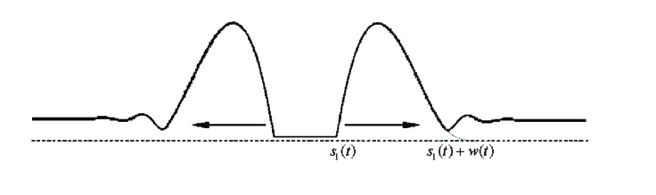
Figure 1: Sketch of the cross-section of a dewetting film after rupture, showing the expanding dewetted residual layer (also called a ’’hole’’ or ’’dry spot’’) in the middle and the adjacent ’’dewetting ridges’’ moving into the surrounding undisturbed uniform film [12].

In the problem at hand, $x=s_{1}(t)$ is the position of the former moving interface, i. e. the contact line, while the position of the latter interface will give an effective measure of the width of the ridge, $x=s_{2}(t)=s_{1}(t)+w(t)$. The ridge is assumed to be moving forward, $\dot{s}_{1}(t)>0$, corresponding to an expanding hole. The arbitrary positive parameter $\theta$ corresponds to the contact angle of liquid-solid interface. Thus, we can control a dewetted region in the film by the contact line and obtain asymmetry profiles of solutions. As the paper [12] has shown that the axisymmetric profile can be analyzed within a one-dimensional thin-film model. The authors found matched asymptotic expansion, speed and structure of the profile, in particular, they obtained that

$$h(x,t)\sim A\,\dot{s_{1}}^{1/2}(s_{2}-x)^{3/2}\text{ at }x=s_{2},$$ (1.4)

where the asymptotic constant $A=2(2/3)^{1/2}$.

Hereinafter, we assume that the contact line moves with a constant velocity (${\rm{v}}$) and the width of the ridge ($w$) is a constant. As in [12], we are going to look for a solution to (1.3) in the following form

$$h(x,t)=\hat{h}(\xi),\text{ where }\xi=x-{\rm{v}}t,\ s_{1}={\rm{v}}t,\ s_{2}={\rm{v}}t+w.$$

We can remove v and $\theta$ from the resulted problem by rescaling appropriately,

$$\hat{h}=\tfrac{\theta^{3}}{\rm{v}}\varphi,\ \xi=\tfrac{\theta^{2}}{{\rm{v}}}\eta,\ w=\tfrac{\theta^{2}}{{\rm{v}}}d.$$

As a result, we obtain the following problem for the traveling-wave

$$\left\{\begin{array}[]{l}\varphi(\eta)\varphi^{\prime\prime\prime}(\eta)=1,\ \varphi(\eta)\geqslant 0,\\ \varphi(0)=\varphi(d)=0,\ \varphi^{\prime}(0)=1,\ 0\leqslant\eta\leqslant d.\\ \end{array}\right.$$ (1.5)

Boatto et al. [8] reduced this problem to the problem of finding a co-dimension one orbit of a second-order ODE system connecting equilibria. Hence generically solutions will exist but only for isolated values of the free parameter $d$. The parameter $d$ was found in [12] by integration (1.5), and

$$d=1/2.$$ (1.6)

Our paper is organized as follows. In Section 2 we prove the existence and uniqueness of a traveling wave solution to the problem (1.5) (Theorem 1). Lower and upper bounds for the traveling wave solution are contained in Section 3 (Theorem 2). We note that the bounds assert that the constant $A$ of (1.4) must be from the interval $[4\sqrt{2}/3,4\sqrt{6}/3]$ (Corollary 3.1). In Section 4 we find an absolute error estimate of approximation of a solution to (1.3) by the traveling-wave solution (Theorem 3).

2 Existence of the traveling wave solution

Below we prove the existence and uniqueness traveling wave solution to the problem (1.5). Our proof is based on some modification of the proof of the existence and uniqueness dipole solutions from [3].

Theorem 1.

There exists a unique solution $\varphi(\eta)$ to the problem (1.5) such that $\varphi(\eta)\in C^{3}(0,d)\cap C^{1}[0,d]$ and $\varphi(\eta)>0$ for $0<\eta<d$.

First, we prove the following auxiliary lemma:

Lemma 2.1.

Assume that $\varphi\in C^{3}(0,d)\cap C^{1}[0,d]$, $\varphi(0)=\varphi(d)=0,\ \varphi^{\prime}(0)=1$, $\varphi>0$ and $\varphi^{\prime\prime\prime}(\eta)\geqslant 0$ in $(0,d)$. Then $\varphi$ has a unique maximum and $\varphi^{\prime}(d)\leqslant 0$.

Proof.

Since $\varphi^{\prime\prime\prime}(\eta)\geqslant 0$ we have that $\varphi^{\prime}(\eta)$ is convex, $\varphi^{\prime\prime}(\eta)$ is increasing. By Rolle’s theorem $\varphi^{\prime}(\eta)$ has at least one zero in $(0,d)$, and $\varphi^{\prime}(\eta)$ has no more than two zeroes in $(0,d)$ by convexity. Let $d_{1},d_{2}\in(0,d):\varphi^{\prime}(d_{1})=\varphi^{\prime}(d_{2})=0$. Then, by Rolle’s theorem, there exists $d_{3}\in(d_{1},d_{2}):\varphi^{\prime\prime}(d_{3})=0$ whence $\varphi(d)\geqslant 0$. In view of $\varphi>0$ in $(0,d)$ and $\varphi(d)=0$, we obtain $d_{2}=d$ and $\varphi^{\prime}(d)=0$. This proves that $\varphi^{\prime}(\eta)$ has exactly one zero in $(0,d)$ and hence $\varphi(\eta)$ has a unique maximum. Now $\varphi^{\prime}(d)<0$ follows easily. ∎

Proof of Theorem 1.

Green’s function. We define a Green’s function $G(\eta,t)$ by

$$\left\{\begin{array}[]{l}G^{\prime\prime\prime}(\eta,t)=\delta(\eta-t),\ 0\leqslant\eta\leqslant d,\ 0\leqslant t\leqslant d,\\ G(0,t)=G(d,0)=G^{\prime}(0,t)=0,\ 0\leqslant t\leqslant d,\\ \end{array}\right.$$ (2.1)

where $d=1/2$. By explicit computation, we find that

$$0\leqslant G(\eta,t)=\left\{\begin{array}[]{l}2(t-d)^{2}\eta^{2}\text{ if }0\leqslant\eta\leqslant t\leqslant d,\\ 2(t-d)^{2}\eta^{2}-d(\eta-t)^{2}\text{ if }0\leqslant t\leqslant\eta\leqslant d,\\ \end{array}\right.$$ (2.2)

whence

$$\int\limits_{0}^{\eta}{G(\eta,t)\,dt}=\tfrac{2}{3}\eta^{3}(d-\eta)(1-\eta),\ \int\limits_{\eta}^{d}{G(\eta,t)\,dt}=\tfrac{2}{3}\eta^{2}(d-\eta)^{3}$$ (2.3)

if $0<\eta<d$, and

$$G(\eta,t)\leqslant C\,t^{2}(d-t),\quad|G^{\prime}(\eta,t)|\leqslant C\,t(d-t)\ \forall\,\eta,\,t\in[0,d].$$ (2.4)

Approximating problems. For each positive integer $k$ we consider the problem

$$\left\{\begin{array}[]{l}\varphi_{k}^{\prime\prime\prime}(\eta)=\varphi_{k}^{-1}\text{ for }0<\eta<d,\\ \varphi_{k}(0)=\varphi_{k}(d)=\frac{1}{k},\ \varphi^{\prime}_{k}(0)=1,\\ \varphi_{k}(\eta)\in C^{3}[0,d],\ \varphi_{k}(\eta)>0\text{ for }0\leqslant\eta\leqslant d.\\ \end{array}\right.$$ (2.5)

Consider the closed convex set

$$S=\{v\in C[0,d]:v\geqslant 1/k\text{ in }(0,d)\}$$

and the nonlinear operator $\Phi_{k}$ defined by

$$\Phi_{k}v(\eta)=\tfrac{1}{k}+2\eta(d-\eta)+\int\limits_{0}^{d}{G(\eta,t)v^{-1}(t)\,dt},$$

where $G(\eta,t)$ is from (2.2). The operator $\Phi_{k}$ mapping $S$ into $S$ is continuous. Moreover, $\Phi_{k}(S)$ is (for each $k$) a bounded subset of $C^{3}[0,d]$ and hence a relatively compact subset of $S$. By Schauder’s fixed-point theorem, there exists $\varphi_{k}\in\Phi_{k}(S)$ such that $\Phi_{k}\varphi_{k}=\varphi_{k}$. This is the desired solution of the problem (2.5). Note that $\varphi_{k}$ satisfies

$$\begin{gathered}\varphi_{k}(\eta)=\tfrac{1}{k}+2\eta(d-\eta)+\int\limits_{0}^{d}{G(\eta,t)\varphi^{\prime\prime\prime}_{k}(t)\,dt},\hfill\\ \varphi^{\prime}_{k}(\eta)=2(d-2\eta)+\int\limits_{0}^{d}{G^{\prime}(\eta,t)\varphi^{\prime\prime\prime}_{k}(t)\,dt}.\hfill\end{gathered}$$ (2.6)

In view of Lemma 2.1 (applied to $\varphi_{k}-1/k$), there exists a unique point $m_{k}$ in which the maximum of $\varphi_{k}$ is attained. Therefore,

$$\varphi_{k}(\eta)\nearrow\text{ in }(0,m_{k})\ \text{and}\ \varphi_{k}(\eta)\searrow\text{ in }(m_{k},d).$$

Estimates. Since $G\geqslant 0$ we get

$$\begin{array}[]{r}\varphi_{k}(\eta)-\frac{1}{k}=2\eta(d-\eta)+\int\limits_{0}^{d}{G(\eta,t)\varphi_{k}^{-1}(t)\,dt}\geqslant\varphi_{k}^{-1}(\eta)\int\limits_{0}^{\eta}{G(\eta,t)\,dt}\\ =\tfrac{2}{3}\eta^{3}(d-\eta)(1-\eta)\varphi_{k}^{-1}(\eta)\geqslant\frac{2}{3}\eta^{3}(d-\eta)^{2}\varphi_{k}^{-1}(\eta),\\ \end{array}$$

whence

$$\varphi_{k}(\eta)\geqslant\sqrt{\tfrac{2}{3}}\eta^{3/2}(d-\eta)\geqslant C\,\eta(d-\eta)^{3/2}\quad{\rm{if}}\quad 0<\eta<m_{k},$$

and

$$\begin{array}[]{r}\varphi_{k}(\eta)-\frac{1}{k}=2\eta(d-\eta)+\int\limits_{0}^{d}{G(\eta,t)\varphi_{k}^{-1}(t)\,dt}\geqslant\varphi_{k}^{-1}(\eta)\int\limits_{\eta}^{d}{G(\eta,t)\,dt}\\ =\tfrac{2}{3}\eta^{2}(d-\eta)^{3}\varphi_{k}^{-1}(\eta),\\ \end{array}$$

whence

$$\varphi_{k}(\eta)\geqslant\sqrt{\tfrac{2}{3}}\eta(d-\eta)^{3/2}\quad{\rm{if}}\quad m_{k}<\eta<d.$$

Hence,

$$\varphi_{k}(\eta)\geqslant C\,\eta(d-\eta)^{3/2}\quad\forall\,\eta\in(0,d).$$ (2.7)

Next we deduce from the differential equation that, for all $\eta\in(0,d)$,

$$\eta(d-\eta)\varphi^{\prime\prime\prime}_{k}(\eta)=\eta(d-\eta)\varphi_{k}^{-1}(\eta)\mathop{\leqslant}\limits^{(\ref{1.6})}C\,(d-\eta)^{-1/2},$$ (2.8)

where the right-hand side is an integrable function.

Passing to the limit. From (2.6), (2.4) and (2.8) it follows that $\varphi_{k}$ is bounded in $C^{1}[0,d]$. Therefore, there exists a subsequence, again denoted by $\varphi_{k}$, and a function $\varphi$ such that $\varphi_{k}\mathop{\to}\varphi$ uniformly on $[0,d]$ as $k\to\infty$. Thus $\varphi(0)=\varphi(d)=0$ and, by (2.7), $\varphi>0$ in $(0,d)$. Hence, for each compact subset $I$ of $(0,d)$ we have

$$\varphi^{\prime\prime\prime}_{k}(\eta)=\varphi_{k}^{-1}(\eta)\mathop{\to}\limits_{k\to\infty}\varphi^{-1}(\eta)\text{ in }C(I),$$

and, by (2.8) and Lebesgue’s dominated convergence theorem,

$$\eta(d-\eta)\varphi^{\prime\prime\prime}_{k}(\eta)\mathop{\to}\limits_{k\to\infty}\eta(d-\eta)\varphi^{-1}(\eta)\text{ in }L^{1}(0,d).$$ (2.9)

Since $\varphi^{\prime\prime\prime}_{k}\mathop{\to}\limits_{k\to\infty}\varphi^{\prime\prime\prime}$ in the distribution sense, it follows that

$$\varphi^{\prime\prime\prime}(\eta)=\varphi^{-1}(\eta)\text{ in }(0,d),$$ (2.10)

i.e. $\varphi$ satisfies the differential equation. Moreover, from (2.9), (2.10), (2.6) and (2.4) we deduce that $\varphi_{k}\mathop{\to}\varphi$ in $C^{1}[0,d]$ as $k\to\infty$, and hence $\varphi$ also satisfies $\varphi^{\prime}(0)=1$. This completes the proof of the existence.

Uniqueness. Let $\varphi_{1}$ and $\varphi_{2}$ be two solutions of the problem (1.5) and set $v=\varphi_{1}-\varphi_{2}$. Since $v^{\prime\prime\prime}=\varphi_{1}^{-1}-\varphi_{2}^{-1}$ and the function $v\mapsto v^{-1}$ is decreasing we deduce that $v\,v^{\prime\prime\prime}\leqslant 0$. Since $v\,v^{\prime\prime\prime}\leqslant 0$ and $v(0)=v(d)=v^{\prime}(0)=0$, we conclude that $v\equiv 0$. This completes the proof of Theorem 1. ∎

3 Lower and upper bounds for the traveling wave solution

Integrating (1.5) with respect to $\eta$, we arrive at the following problem

$$\left\{\begin{array}[]{l}\varphi(\eta)\varphi^{\prime\prime}(\eta)=\tfrac{1}{2}(\varphi^{\prime}(\eta))^{2}+\eta-d,\ \varphi(\eta)\geqslant 0,\\ \varphi(0)=0,\,\varphi^{\prime}(0)=1,\ 0\leqslant\eta\leqslant d,\\ \end{array}\right.$$ (3.1)

where $d$ is from (1.6). Analyzing the behaviour of a solution to (3.1), we find explicit lower and upper bounds for the solution.

Theorem 2.

Let $\varphi(\eta)$ be a solution from Theorem 1. Then the following estimates are valid

$$\varphi_{\min}(\eta)\leqslant\varphi(\eta)\leqslant\varphi_{\max}(\eta)\Leftrightarrow\tfrac{4\sqrt{2}}{3}\eta(d-\eta)^{3/2}\leqslant\varphi(\eta)\leqslant\tfrac{{4\sqrt{6}}}{3}\,\eta(d-\eta)^{3/2}$$ (3.2)

for all $\eta\in[0,d]$ $($see Figure 2$)$.

Corollary 3.1.

In particular, from (3.2) it follows that

$$\tfrac{4\sqrt{2}}{3}\dot{s}_{1}^{1/2}\tfrac{x-s_{1}}{s_{2}-s_{1}}(s_{2}-x)^{3/2}\leqslant h(x,t)\leqslant\tfrac{4\sqrt{6}}{3}\dot{s}_{1}^{1/2}\tfrac{x-s_{1}}{s_{2}-s_{1}}(s_{2}-x)^{3/2}$$ (3.3)

for all $x\in[s_{1},s_{2}]$.

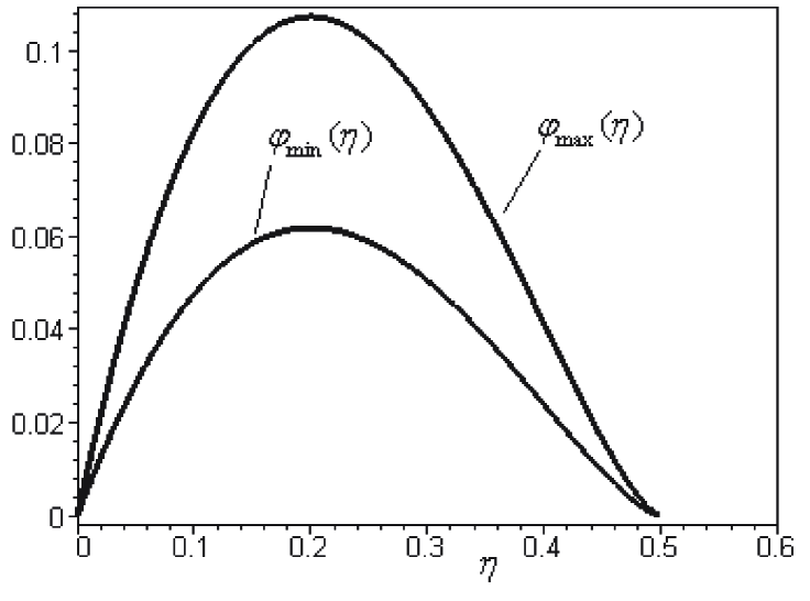
Figure 2: Lower and upper bounds for the traveling wave solution

Lemma 3.1.

The function $\varphi_{0}(\eta)=A_{0}\,\eta(d-\eta)^{3/2}$ $(A_{0}>0)$ satisfies the inequalities

$$\varphi\varphi^{\prime\prime}\geqslant\tfrac{1}{2}(\varphi^{\prime})^{2}+\eta-d\ \forall\,\eta\in[0,d]\text{ if }A_{0}^{2}d^{2}\leqslant 5/3,$$ (3.4)

$$\varphi\varphi^{\prime\prime}\leqslant\tfrac{1}{2}(\varphi^{\prime})^{2}+\eta-d\ \forall\,\eta\in[0,d]\text{ if }A_{0}^{2}d^{2}\geqslant 8/3.$$ (3.5)

Proof.

Indeed, the function $\varphi_{0}(\eta)$ satisfies the equation

$$\varphi_{0}\varphi^{\prime\prime}_{0}=\tfrac{1}{2}(\varphi^{\prime}_{0})^{2}+f(\eta),$$

where

$$f(\eta):=\tfrac{5}{8}A_{0}^{2}(d-\eta)\left({\eta-\tfrac{2d(1-\sqrt{6})}{5}}\right)\left({\eta-\tfrac{2d(1+\sqrt{6})}{5}}\right)\leqslant 0\ \forall\,\eta\in[0,d].$$

From

$$f(\eta)\geqslant\eta-d\Leftrightarrow 5\eta^{2}-4d\eta-4d^{2}+\tfrac{8}{A_{0}^{2}}\geqslant 0\ \forall\,\eta\in[0,d],$$

$$D=4d^{2}+20d^{2}-\tfrac{40}{A_{0}^{2}}=\tfrac{24}{A_{0}^{2}}\left({A_{0}^{2}d^{2}-\tfrac{5}{3}}\right)\leqslant 0\text{ if }A_{0}^{2}d^{2}\leqslant 5/3$$

we obtain (3.4). In a similar way, we obtain (3.5) for $f(\eta)\leqslant\eta-d$ $\forall\,\eta\in[0,d]$ if $A_{0}^{2}d^{2}\geqslant 8/3$. ∎

Lemma 3.2.

The function $\varphi_{\min}(\eta)=A_{1}\eta(d-\eta)^{3/2}$ $(A_{1}>0)$ if $A_{1}^{2}d^{2}\leqslant 8/9$ is a lower bound for the solution $\varphi(\eta)$ of (3.1)$:$

$$\varphi_{\min}(\eta)\leqslant\varphi(\eta)\ (\text{i.\,e. }\varphi_{\min}(\eta)-\varphi(\eta)\leqslant 0)\ \forall\,\eta\in[0,d].$$

Proof.

’’Contraction Principle’’. Let us define $v(\eta):=\varphi_{\min}(\eta)-\varphi(\eta)$. Suppose that there exists a point $\eta_{0}\in[0,d]$ such that $v(\eta_{0})>0$ then $\eta_{0}$ is a point of maximum for $v(\eta)$, i. e. $v^{\prime}(\eta_{0})=0\Leftrightarrow\varphi^{\prime}_{\min}(\eta_{0})=\varphi^{\prime}(\eta_{0})=M$ and $v^{\prime\prime}(\eta_{0})<0$. From (3.1) and (3.4) we deduce that

$$\left\{\begin{array}[]{l}\varphi\varphi^{\prime\prime}=\tfrac{1}{2}(\varphi^{\prime})^{2}+\eta-d\\ \varphi_{\min}\varphi^{\prime\prime}_{\min}\geqslant\tfrac{1}{2}(\varphi^{\prime}_{\min})^{2}+\eta-d\\ \end{array}\right.\Rightarrow$$

$$v^{\prime\prime}(\eta)\geqslant\tfrac{1}{2}\left({\tfrac{(\varphi_{\min,\eta})^{2}}{\varphi_{\min}}-\tfrac{(\varphi_{\eta})^{2}}{\varphi}}\right)+(\eta-d)\left({\tfrac{1}{\varphi_{\min}}-\tfrac{1}{\varphi}}\right),$$

whence

$$\underbrace{v^{\prime\prime}(\eta_{0})}_{<0}\geqslant\underbrace{\tfrac{-v(\eta_{0})}{\varphi_{\min}(\eta_{0})\varphi(\eta_{0})}}_{<0}\underbrace{\left({\tfrac{1}{2}M^{2}+\eta_{0}-d}\right)}_{?}.$$

Using $M=A_{1}(d-\eta_{0})^{1/2}(d-5\eta_{0}/2)$, we find

$$\tfrac{1}{2}M^{2}+\eta_{0}-d=(d-\eta_{0})\bigl{[}\tfrac{1}{2}A_{1}^{2}(d-5\eta_{0}/2)^{2}-1\bigr{]}\leqslant 0\ \forall\,\eta_{0}\in[0,d]\text{ if }A_{1}^{2}d^{2}\leqslant 8/9.$$

Thus we obtain a contradiction with our assumption, which proves the assertion of Lemma 3.2. ∎

Lemma 3.3.

The function $\varphi_{\max}(\eta)=A_{2}\,\eta(d-\eta)^{3/2}$ $(A_{2}>0)$ if $A_{2}^{2}d^{2}\geqslant 8/3$ is an upper bound for the solution $\varphi(\eta)$ of (3.1)$:$

$$\varphi(\eta)\leqslant\varphi_{\max}(\eta)\ (\text{i.\,e. }\varphi(\eta)-\varphi_{\max}(\eta)\leqslant 0)\ \forall\eta\in[0,d].$$

Proof.

’’Contraction Principle’’. Let us define $v(\eta):=\varphi(\eta)-\varphi_{\max}(\eta)$. Suppose that there exists a point $\eta_{0}\in[0,d]$ such that $v(\eta_{0})>0$ then $\eta_{0}$ is a point of maximum for $v(\eta)$, i. e. $v^{\prime}(\eta_{0})=0\Leftrightarrow\varphi^{\prime}_{\max}(\eta_{0})=\varphi^{\prime}(\eta_{0})$ and $v^{\prime\prime}(\eta_{0})<0$. Moreover, from $\varphi^{\prime\prime}_{\max}(\eta)=3A_{1}(d-\eta)^{-1/2}[5\eta/4-d]$ we find that $\varphi^{\prime\prime}_{\max}(\eta)\leqslant 0$ for all $\eta\in[0,0.4]$ and $\varphi^{\prime\prime}_{\max}(\eta)>0$ for all $\eta\in(0.4,d]$. From (3.1) and (3.5) we deduce that

$$\left\{\begin{array}[]{l}\varphi\varphi^{\prime\prime}=\tfrac{1}{2}(\varphi^{\prime})^{2}+\eta-d\\ \varphi_{\max}\varphi^{\prime\prime}_{\max}\leqslant\tfrac{1}{2}(\varphi^{\prime}_{\max})^{2}+\eta-d\\ \end{array}\right.\Rightarrow\varphi(\eta_{0})\varphi^{\prime\prime}(\eta_{0})-\varphi_{\max}(\eta_{0})\varphi^{\prime\prime}_{\max}(\eta_{0})\geqslant 0,$$ (3.6)

whence

$$\underbrace{\varphi(\eta_{0})\varphi^{\prime\prime}(\eta_{0})-\varphi_{\max}(\eta_{0})\,\varphi^{\prime\prime}_{\max}(\eta_{0})}_{\geqslant 0}=\underbrace{\varphi(\eta_{0})v^{\prime\prime}(\eta_{0})}_{\leqslant 0}+\underbrace{\varphi^{\prime\prime}_{\max}(\eta_{0})\,v(\eta_{0})}_{\leqslant 0}.$$

This contradicts to our assumption if $\eta_{0}\in[0,0.4]$.

Now, let $\eta_{0}\in(0.4,d]$. In this case, if $\varphi^{\prime\prime}(\eta_{0})\leqslant 0$, and we obtain a contradiction immediately from (3.6). If $\varphi^{\prime\prime}(\eta_{0})>0$ then we rewrite (3.6) in equivalent form:

$$\left\{\begin{array}[]{l}\tfrac{1}{2}(\varphi^{2})^{\prime\prime}=\frac{3}{2}(\varphi^{\prime})^{2}+\eta-d\\ \tfrac{1}{2}(\varphi_{\max}^{2})^{\prime\prime}\leqslant\tfrac{3}{2}(\varphi^{\prime}_{\max})^{2}+\eta-d\\ \end{array}\right.\Rightarrow(\varphi^{2}(\eta_{0})-\varphi_{\max}^{2}(\eta_{0}))^{\prime\prime}\geqslant 0,$$ (3.7)

whence

$$\underbrace{(\varphi^{2}(\eta_{0})-\varphi_{\max}^{2}(\eta_{0}))^{\prime\prime}}_{\geqslant 0}=\underbrace{(\varphi^{\prime\prime}(\eta_{0})+\varphi^{\prime\prime}_{\max}(\eta_{0}))}_{>0}\underbrace{v^{\prime\prime}(\eta_{0})}_{<0}$$

and we arrive at a contradiction. Thus, Lemma 3.3 is proved. ∎

As a result of Lemmata 3.2 and 3.3, we obtain lower (more exact in comparison with (2.7)) and upper bounds for the solution of (3.1), and consequently for the solution of (1.5).

4 Absolute error estimate of approximation of a solution by a traveling-wave solution

The next theorem contains an absolute error estimate of approximation of a solution (e.g., a generalized solution) by a traveling-wave solution.

Theorem 3.

Let $h(x,t)$ be a solution and $\hat{h}(\xi)$ be the traveling-wave solution to the problem (1.3). Then the following estimates hold

$$\begin{array}[]{l}\mathop{\sup}\limits_{x\in[s_{1},s_{2}]}|{h(x,t)-\hat{h}(\xi)}|\leqslant\tfrac{\sqrt{6}}{6}\theta(s_{2}-s_{1})^{1/2}\text{ if }|h_{x}(s_{2})|>\theta,\\ \mathop{\sup}\limits_{x\in[s_{1},s_{2}]}\!\!\!\bigl{|}h(x,t)-\hat{h}(\xi)-2\theta s_{1}^{1/2}\!(s_{2}-s_{1})^{1/2}\bigr{|}\!\leqslant\!\tfrac{\sqrt{6}}{6}\theta(s_{2}-s_{1})^{1/2}\text{ if }|h_{x}(s_{2})|\leqslant\theta,\\ \end{array}$$ (4.1)

where $\xi=x-{\rm{v}}t,\ s_{1}={\rm{v}}t$ and $s_{2}=s_{1}+w$.

Proof of Theorem 3.

We make the following change of variables in (1.3)

$$h(x,t)\mapsto f(\xi,t),\text{ where }\xi=x-{\rm{v}}t.$$

As a result, we obtain the following problem

$$\left\{\begin{array}[]{l}f_{t}-{\rm{v}}\,f_{\xi}+(f^{2}f_{\xi\xi\xi})_{\xi}=0,\\ f(0,t)=f(w,t)=0,\quad f^{2}f_{\xi\xi\xi}=0\text{ at }\xi=0,\\ f_{\xi}(0,t)=\theta>0.\\ \end{array}\right.$$ (4.2)

Multiplying (4.2₁) by $-f_{\xi\xi}(\xi,t)$ and integrating with respect to $\xi$, we get

$$\begin{array}[]{c}\tfrac{1}{2}\tfrac{d}{dt}\int\limits_{0}^{w}{f_{\xi}^{2}(\xi,t)\,d\xi}=-{\rm{v}}\int\limits_{0}^{w}{f_{\xi}f_{\xi\xi}\,d\xi}+\int\limits_{0}^{w}{(f^{2}f_{\xi\xi\xi})_{\xi}f_{\xi\xi}\,d\xi}=-\tfrac{{\rm{v}}}{2}\int\limits_{0}^{w}{\tfrac{\partial}{\partial\xi}(f_{\xi}^{2})\,d\xi}+\\ +\int\limits_{0}^{w}{(f^{2}f_{\xi\xi\xi})_{\xi}f_{\xi\xi}\,d\xi}\mathop{=}\limits^{(\ref{3.2}_{2}),(\ref{3.2}_{3})}\tfrac{\rm{v}}{2}(\theta^{2}-f_{\xi}^{2}(w,t))-\int\limits_{0}^{w}{f^{2}f_{\xi\xi\xi}^{2}\,d\xi},\end{array}$$

whence

$$\tfrac{1}{2}\tfrac{d}{dt}\int\limits_{0}^{w}{f_{\xi}^{2}(\xi,t)\,d\xi}+\int\limits_{0}^{w}{f^{2}f_{\xi\xi\xi}^{2}\,d\xi}=\tfrac{\rm{v}}{2}(\theta^{2}-f_{\xi}^{2}(w,t))\Rightarrow\\ \tfrac{d}{dt}\int\limits_{0}^{w}{f_{\xi}^{2}(\xi,t)\,d\xi}\leqslant{\rm{v}}(\theta^{2}-f_{\xi}^{2}(w,t)).$$ (4.3)

Integrating (4.3) with respect to time, we find

$$\|{f_{\xi}(\xi,t)}\|_{L^{2}(0,w)}^{2}\leqslant\|{f_{\xi}(\xi,0)}\|_{L^{2}(0,w)}^{2}+{\rm{v}}\int\limits_{0}^{t}{(\theta^{2}-f_{\xi}^{2}(w,t))\,dt}.$$ (4.4)

From (4.4) it follows that

$$\left\|{f_{\xi}(\xi,t)}\right\|_{L^{2}(0,w)}^{2}\leqslant\left\{\begin{array}[]{c}\left\|{f_{\xi}(\xi,0)}\right\|_{L^{2}(0,w)}^{2}\text{ if }|f_{\xi}(w,t)|>\theta,\\ \left\|{f_{\xi}(\xi,0)}\right\|_{L^{2}(0,w)}^{2}+{\rm{v}}\theta^{2}t\text{ if }|f_{\xi}(w,t)|\leqslant\theta.\\ \end{array}\right.$$ (4.5)

From this, by virtue of uniqueness of the traveling-wave solution $\hat{h}(\xi)$ (see Theorem 1), $f(\xi,0)=\hat{h}(\xi)$ we deduce from (4.5) that

$$\begin{array}[]{l}\|{f_{\xi}(\xi,t)-\hat{h}_{\xi}(\xi)}\|_{L^{2}(0,w)}\leqslant 2\|{\hat{h}_{\xi}(\xi)}\|_{L^{2}(0,w)}\text{ if }|f_{\xi}(w,t)|>\theta,\\ \|{f_{\xi}(\xi,t)-\hat{h}_{\xi}(\xi)}\|_{L^{2}(0,w)}\leqslant 2\|{\hat{h}_{\xi}(\xi)}\|_{L^{2}(0,w)}+2\theta\sqrt{{\rm{v}}\,t}\text{ if }|f_{\xi}(w,t)|\leqslant\theta.\\ \end{array}$$

Therefore taking into account the embedding $\mathop{H^{1}}\limits^{o}(0,w)\subset C[0,w]$, we find that

$$\begin{gathered}\mathop{\sup}\limits_{\xi\in[0,w]}|{f(\xi,t)-\hat{h}(\xi)}|\leqslant 2w^{1/2}\|{\hat{h}_{\xi}(\xi)}\|_{L^{2}(0,w)}\text{ if }|f_{\xi}(w,t)|>\theta,\hfill\\ \mathop{\sup}\limits_{\xi\in[0,w]}|f(\xi,t)-\hat{h}(\xi)|\leqslant 2w^{1/2}(\|{\hat{h}_{\xi}(\xi)}\|_{L^{2}(0,w)}+\theta\sqrt{{\rm{v}}\,t})\text{ if }|f_{\xi}(w,t)|\leqslant\theta.\hfill\end{gathered}$$ (4.6)

Since $\hat{h}_{\xi}(\xi)=\theta\varphi^{\prime}_{\eta}(\eta)$ ($\varphi(\eta)$ is from Theorem 1) and $\varphi(\eta)$ has a unique maximum in $(0,d)$, due to (3.2) we conclude that

$$\|{\hat{h}_{\xi}(\xi)}\|_{L^{2}(0,w)}\leqslant\tfrac{\sqrt{6}}{12}\theta.$$ (4.7)

Thus, we from (4.6) and (4.7) arrive at

$$\begin{gathered}\mathop{\sup}\limits_{\xi\in[0,w]}|{f(\xi,t)-\hat{h}(\xi)}|\leqslant\tfrac{\sqrt{6}}{6}\theta w^{1/2}\text{ if }|f_{\xi}(w,t)|>\theta,\hfill\\ \mathop{\sup}\limits_{\xi\in[0,w]}|f(\xi,t)-\hat{h}(\xi)-2\theta w^{1/2}\sqrt{{\rm{v}}\,t}|\leqslant\tfrac{\sqrt{6}}{6}\theta w^{1/2}\text{ if }|f_{\xi}(w,t)|\leqslant\theta,\hfill\end{gathered}$$ (4.8)

which completes the proof of Theorem 3. ∎

Acknowledgement. Author would like to thank to Andreas Münch for his valuable comments and remarks. Research is partially supported by the INTAS project Ref. No: 05-1000008-7921.

References

- [1] E. Beretta, M. Bertsch, R. Dal Passo, Nonnegative solutions of a fourth-order nonlinear degenerate parabolic equation, Arch. Rat. Mech. Anal. 129 (1995) 175–200.
- [2] F. Bernis, A. Friedman, Higher order nonlinear degenerate parabolic equations, J. Diff. Equ. 83 (1990) 179–206.
- [3] F. Bernis, J. Hulshof, J.R. King, Dipoles and similarity solutions of the thin film equatoin in the half–line, Nonlinearity 13 (2000) 413–439.
- [4] F. Bernis, L.A. Peletier, S.M. Williams, Source type solutions of a fourth order nonlinear degenerate parabolic equation, Nonlinear Anal. TMA. 18 (3) (1992) 217–234.
- [5] A.L. Bertozzi, M.P. Brenner, Linear stability and transient growth in driven contact lines, Phys. Fluids 9(3) (1997) 530–539.
- [6] A.L. Bertozzi, M.P. Brenner, T.F. Dupont, L.P. Kadanoff, Singularities and similarities in interface flows, in: Trends and perspectives in applied mathematics, Appl. Math. Sci., Vol. 100, Springer, New York, 1994, 155–208.
- [7] A.L. Bertozzi, M. Pugh, The lubrication approximation for thin viscous films: the moving contact line with a porous media cutoff of the Van der Waals interactions, Nonlinearity 7 (1994) 1535–1564.
- [8] S. Boatto, L.P. Kadanoff, P. Olla, Traveling-wave solutions to thin-film equations, Phys. Rev. E 48(6) (1993) 4423–4431.
- [9] L. Giacomelli, F. Otto, Rigorous lubrication approximation, Interfaces Free Bound. 5 (4) (2003) 483–529.
- [10] D.E. Kataoka, S.M. Troian, A theoretical study of instabilities at the advancing front of thermally driven coating films, J. Coll. Interf. Sci. 192 (1997) 350–362.
- [11] J.R. King, A. Münch, B. Wagner, Linear stability of a ridge, Nonlinearity 19(12) (2006) 2813–2831.
- [12] A. Münch, B. Wagner, T.P. Witelski, Lubrication models with small to large slip lengths, J. Engrg. Math. 53(3-4) (2005) 359–383.
- [13] A. Oron, S.H. Davis, S.G. Bankoff, Long-scale evolution of thin liquid films, Rev. Mod. Phys. 69 (1997) 931–980.