Effects of the quantization ambiguities on the Big Bounce dynamics

Abstract

In this paper we investigate dynamics of the modified loop quantum cosmology models using dynamical systems methods. Modifications considered come from the choice of the different field strength operator $\hat{F}$ and result in different forms of the effective Hamiltonian. Such an ambiguity of the choice of this expression from some class of functions is allowed in the framework of loop quantization. Our main goal is to show how such modifications can influence the bouncing universe scenario in the loop quantum cosmology. In effective models considered we classify all evolutional paths for all admissible initial conditions. The dynamics is reduced to the form of a dynamical system of the Newtonian type on a 2-dimensional phase plane. These models are equivalent dynamically to the FRW models with the decaying effective cosmological term parameterized by the canonical variable $p$ (or by the scale factor $a$). We demonstrate that the evolutional scenario depends on the geometrical constant parameter $\Lambda$ as well as the model parameter $n$. We find that for the positive cosmological constant there is a class of oscillating models without the initial and final singularities. The new phenomenon is the appearance of curvature singularities for the finite values of the scale factor, but we find that for the positive cosmological constant these singularities can be avoided. The values of the parameter $n$ and the cosmological constant differentiate asymptotic states of the evolution. For the positive cosmological constant the evolution begins at the asymptotic state in the past represented by the de Sitter contracting (deS_-) spacetime or the static Einstein universe $H=0$ or $H=-\infty$ state and reaches the de Sitter expanding state (deS₊), the state $H=0$ or $H=+\infty$ state. In the case of the negative cosmological constant we obtain the past and future asymptotic states as the Einstein static universes.

I Introduction

According to the General Relativity the initial state of the universe was a causal singularity. In this point all time-like geodesics were cut off and has no extension into the past. This peculiar behaviour corresponds to the blow up of the curvature $\mathcal{R}\rightarrow\infty$ and energy density $\rho\rightarrow\infty$ in the standard Big-Bang scenario. It is however believed that singularities of this kind are not real states but rather artifacts resulting from the fact that classical theory broke down. In the vicinity of the initial singularity, when the universe reaches the Planck scale energy, the quantum gravity effects were proposed as a mechanism to remove the singular behaviour. Such a possibility was studied in the context of the String Theory leading to the so called pre-Big Bang cosmological scenario Gasperini and Veneziano (2007). Presently this issue is also studied extensively in the Loop Quantum Cosmology (LQC)Bojowald (2005) where the avoidance of the initial singularity appeared in a natural way Bojowald (2007a). This approach possesses other advantages like the adjustment of the proper initial conditions for the inflationary phase. The avoidance of the initial singularity appeared here in the form of the non-singular bouncing universe Ashtekar et al. (2006a); Bojowald (2007b). Namely, the universe is initially in the contracting phase, then reaches a minimal nonzero volume and due to quantum repulsion evolves toward an expanding phase. It should be stressed that this result has been strictly demonstrated so far only for isotropic models with a free, massless scalar field Ashtekar et al. (2006b). The phenomenological dynamics of this scenario has been extensively studied Singh et al. (2006); Mielczarek et al. (2008). However ambiguities in the quantization of the classical formula lead to some deviations. In the frame of the standard quantization scheme these ambiguities lead generally to the models with qualitatively similar bouncing behaviour. However like it was shown in Mielczarek et al. (2008), for some special setup in the effective flat FRW model the bounce is replaced by non-singular oscillations. More drastic consequences appear when we choose the different quantization framework. This issue was studied in Mielczarek and Szydlowski (2008) and it was found the existence of the finite scale factor curvature singularities in the co-existence with a quantum bounce. In this paper we continue these studies in the nonstandard quantization frameworks. We investigate the effects of resulting ambiguities for the dynamics of the effective FRW models with the cosmological constant. We present simple methods of reducing dynamical equation governing evolution of the models with quantum corrections to the form of a 2-dimensional autonomous dynamical system of the Newtonian type. We explore a mechanical analogy in investigation of different evolutionary scenarios.

The organization of the text is the following. In section II we investigate possible kinds of ambiguities in the loop quantization, concentrating on the expression for the field strength operator $\hat{F}$. Next, in section III we investigate resulting cosmological models with use of the qualitative methods analysis of dynamics. In section V we summarize the results.

II Field strength operator $\hat{F}$ and quantization ambiguities

This section aims to summarize some key features of loop quantization of cosmological models and discusses arising ambiguities. In particular we extend study of the choice of the field strength operator $\hat{F}$ began in Mielczarek and Szydlowski (2008). We restrict our consideration to the flat FRW cosmological models which are given by the metric

$$ds^{2}=-N^{2}(x)dt^{2}+q_{ab}dx^{a}dx^{b}$$ (1)

where $N(x)$ is the lapse function and the spatial part of the metric is expressed as

$$q_{ab}=\delta_{ij}{\omega^{i}_{a}}{\omega^{j}_{b}}=a^{2}(t){{}^{o}q}_{ab}=a^{2}(t)\delta_{ij}{{}^{o}\omega^{i}_{a}}{{}^{o}\omega^{j}_{b}}.$$ (2)

In this expression ${{}^{o}q}_{ab}$ is the fiducial metric and ${{}^{o}\omega^{i}_{a}}$ are the co-triads dual to the triads ${{}^{o}e^{a}_{i}}$, ${{}^{o}\omega^{i}}({{}^{o}e_{j}})=\delta^{i}_{j}$ where ${}^{o}\omega^{i}={{}^{o}\omega^{i}_{a}}dx^{a}$ and ${}^{o}e_{i}={{}^{o}e_{i}^{a}}\partial_{a}$. Based on the triads we can construct the Ashtekar variables

$$A^{i}_{a} \equiv \Gamma^{i}_{a}+\gamma K_{a}^{i}=cV_{0}^{-1/3}\ {{}^{o}\omega^{i}_{a}},$$ (3)

$$E^{a}_{i} \equiv \sqrt{|\det q|}e^{a}_{i}=pV_{0}^{-2/3}\sqrt{{}^{o}q}\ {{}^{o}e^{a}_{i}}$$ (4)

where

$$|p| = a^{2}V_{0}^{2/3},$$ (5)

$$c = \gamma\dot{a}V_{0}^{1/3}.$$ (6)

The volume $V_{0}$ is the so called fiducial cell and is introduced to perform the integration on the non-compact spaces. We expect that the physical results should not depend on its value. However, when we introduce quantum modifications in general they can depend on the choice of $V_{0}$.

In loop quantum cosmology we consider effects of the inverse volume corrections and holonomies. In the phenomenological considerations of the quantized FRW $k=0$ model it is appropriate to take into account quantum modifications arising only from the field strength expressed in terms of holonomies. In some special case ($n=-1/2$) this kind of modification does not depend on the choice of the fiducial cell $V_{0}$. This simplifies interpretation of results and make the correspondence with classical physics easier. This issue is related to the question of the loop quantization uniqueness of the cosmological models Corichi and Singh (2008). Because there is no defined length scale in the flat FRW models the $V_{0}$ dependence seems to be unphysical. This problem is not present in the FRW $k=\pm 1$ models, where the length scale is tied with the intrinsic curvature Ashtekar et al. (2007).

The loop quantization requires to replace the classical variables by the quantum operators expressed in terms of the holonomies and fluxes. In the FRW models holonomies reduce to almost periodic functions $\sum_{j}\xi_{j}e^{i\mu_{j}c/2}$ and fluxes reduce to variable $p$ multiplied by the kinematic factor Ashtekar et al. (2003). Then algebra of variables $p$ and $e^{i\mu c/2}$ is quantized. The quantum Poisson bracket of elementary operators is

$$\left[\hat{p},\widehat{e^{\frac{i\mu c}{2}}}\right]=\mu\frac{8\pi l_{\text{Pl}}^{2}\gamma}{6}\widehat{e^{\frac{i\mu c}{2}}}$$ (7)

and these operators act in the Hilbert space $L^{2}(\mathbb{R}_{\text{Bohr}},d\mu_{\text{Bohr}})$. The basis of this space can be chosen as a set of eigenstates of the operator $\hat{p}$

$$\hat{p}|\mu\rangle=\mu\frac{8\pi\gamma l^{2}_{\text{Pl}}}{6}|\mu\rangle$$ (8)

which fulfils the normalization condition $\langle\mu|\mu^{\prime}\rangle=\delta_{\mu,\mu^{\prime}}$. The action of the operator $\hat{N}=\widehat{e^{\frac{i\mu c}{2}}}$ is following

$$\widehat{e^{\frac{i\mu c}{2}}}|\mu^{\prime}\rangle=|\mu^{\prime}+\mu\rangle.$$ (9)

We have defined a quantum kinematic sector of the loop quantum cosmology. Now with use of these rules we aim to quantize the scalar constraint

$$\mathcal{H}_{\rm G}=\frac{1}{16\pi G}\int_{\Sigma}d^{3}xN(x)\frac{E^{a}_{i}E^{b}_{j}}{\sqrt{|\mathrm{det}E|}}\left[{\varepsilon^{ij}}_{k}F_{ab}^{k}-2(1+\gamma^{2})K^{i}_{[a}K^{j}_{b]}\right]$$ (10)

where the extrinsic curvature is defined as

$$K_{ab}=\frac{1}{2N}\left[\dot{q}_{ab}-2D_{(a}N_{b)}\right]$$ (11)

which corresponds to $K^{i}_{a}:=K_{ab}e^{b}_{i}$. The scalar constraint quantum operator should be expressed in terms of the elementary operators $\hat{p}$ and $\hat{N}=\widehat{e^{\frac{i\mu c}{2}}}$. In our considerations we restrict ourselves to quantization of the field strength $F_{ab}^{k}$. The rest of the terms lead to quantum operators expressed in term of the inverse volume operator. Detailed analysis of the scalar constraint quantization can be found in Vandersloot (2005).

As we have said our main interest is to find a formula for the field strength operator $\hat{F}$. The standard approach to introduce this operator is to consider a closed path $\alpha=\Box_{ij}\in\Sigma$ and holonomy along this loop. Such a holonomy can be written as

$$h_{\Box_{ij}}^{(\mu)}=h_{i}^{(\mu)}h_{j}^{(\mu)}h_{i}^{(\mu)-1}h_{j}^{(\mu)-1}$$ (12)

where particular holonomies are

$$h_{i}^{(\mu)}=e^{\tau_{i}\mu c}=\mathbb{I}\cos\left(\frac{\mu c}{2}\right)+2\tau_{i}\sin\left(\frac{\mu c}{2}\right).$$ (13)

With use of the above expressions one can derive formula

$$F^{k}_{ab}=-2\frac{\text{tr}\left[\tau_{k}\left(h^{(\mu)}_{\Box_{ij}}-\mathbb{I}\right)\right]}{\mu^{2}V_{0}^{2/3}}{{}^{o}\omega^{i}_{a}}{{}^{o}\omega^{j}_{b}}+\frac{\mathcal{O}(\mu^{4})}{\mu^{2}}.$$ (14)

Based on this expression we can define the quantum field strength operator. However, we should discuss some related issues. Firstly, quantization of the area operator in the Loop Quantum Gravity leads to the existence of the area gap $\text{Ar}_{\text{min}}=\Delta$ Ashtekar and Lewandowski (1997). This means that the limit $\text{Ar}_{\Box_{ij}}\rightarrow 0$ of the area enclosed by the loop does not exist. We should stop shrinking the loop at a minimal area which is related to limiting $\mu\rightarrow\bar{\mu}$ value. This process is however ambiguous and generally limiting $\mu$ can have a form

$$\bar{\mu}=\xi|p|^{n}$$ (15)

where $n\in[-1/2,0)$ Bojowald (2008) and $\xi$ is dimension-full and positive real parameter. In particular, from this expression we can recover known $\bar{\mu}$-scheme for which

$$\bar{\mu}=\sqrt{\frac{\Delta}{|p|}}.$$ (16)

In this case the area gap $\Delta$ corresponds to the physical area of the loop $|p|\bar{\mu}^{2}$. The range of the $n$ parameter written above can be obtained from the considerations of the lattice states Bojowald (2006). Further restrictions for value of this parameter come from considerations of the anomaly cancellation in the inhomogeneous cosmological models and positivity of the graviton effective mass, giving $-0.1319>n\geq-5/2$ Bojowald and Hossain (2008).

The properties considered should be now taken into account during the construction of the operator $\hat{F}$. The standard procedure is to cut-off the terms $\mathcal{O}(\mu^{4})$ and perform the limit $\text{Ar}\rightarrow\Delta$ in expression (14), what gives Ashtekar et al. (2006c)

$$\hat{F}^{k}_{ab}=-2\lim_{\text{Ar}\rightarrow\Delta}\frac{\text{tr}\left[\tau_{k}\left(h^{(\mu)}_{\Box_{ij}}-\mathbb{I}\right)\right]}{\mu^{2}V_{0}^{2/3}}{{}^{o}\omega^{i}_{a}}{{}^{o}\omega^{j}_{b}}=\frac{\sin^{2}\left(\bar{\mu}c\right)}{\bar{\mu}^{2}V_{0}^{2/3}}\epsilon_{kij}{{}^{o}\omega^{i}_{a}}{{}^{o}\omega^{j}_{b}}.$$ (17)

This is the well defined operator on the Hilbert space $L^{2}(\mathbb{R}_{\text{Bohr}},d\mu_{\text{Bohr}})$. Namely, due to relation $\sin\left(\bar{\mu}c\right)=\frac{1}{2i}\left(e^{i\bar{\mu}c}-e^{-i\bar{\mu}c}\right)$ it can be expressed in terms of the operator $\hat{N}$ and due to the power-low $\bar{\mu}(p)$ dependence this part can be expressed in terms of the operator $\hat{p}$. The proper classical behaviour is also obtained, it means that no information about classical expression is contained in the terms $\mathcal{O}(\mu^{4})$. These terms simply vanish in the classical limit $\mu\rightarrow 0$, $\mathcal{O}(\mu^{4})\rightarrow 0$. Another motivation to consider (17) as a proper quantum operator is the resulting dynamics. Namely, this quantum operator leads to the avoidance of the initial singularity.

However we can ask what happens when a part of the $\mathcal{O}(\mu^{4})$ contribute to the definition of the operator $\hat{F}$? The resulting operator has proper classical behaviour, because the contribution from $\mathcal{O}(\mu^{4})$ vanishes in the classical limit. However on the quantum level the operator $\hat{F}$ contain some new terms which influence quantum dynamics. It is worth to stress this property. This additional modification term, which influence dynamics in the quantum regime, does not correspond to any contribution on the classical level. The possibility of existence of such terms lead to the ambiguity in the definition of the operator $\hat{F}$. However not all modifications which fulfil well the classical limit are allowed. Another property which must hold is that the resulting operator must be defined on the Hilbert space $L^{2}(\mathbb{R}_{\text{Bohr}},d\mu_{\text{Bohr}})$.

In the paper Mielczarek and Szydlowski (2008) the expression for the $\hat{F}$ operator including the term $\mathcal{O}(\mu^{4})$ was calculated

$$\hat{F}_{ab}^{k}=\epsilon^{k}_{\ ij}\frac{1-\sqrt{1-\frac{4}{3}\sin^{2}\left(\bar{\mu}c\right)}}{\frac{2}{3}\bar{\mu}^{2}V_{0}^{2/3}}{{}^{o}\omega^{i}_{a}}{{}^{o}\omega^{j}_{b}}.$$ (18)

Expanding the square we obtain

$$\frac{1-\sqrt{1-\frac{4}{3}\sin^{2}\left(\bar{\mu}c\right)}}{\frac{2}{3}\bar{\mu}^{2}}=\left[\frac{\sin(\bar{\mu}c)}{\bar{\mu}}\right]^{2}+\frac{1}{3}\frac{\sin^{4}(\bar{\mu}c)}{\bar{\mu}^{2}}+\dots.$$ (19)

We see that the first term in this series corresponds to the standard field strength operator. Other parts vanish in the limit $\bar{\mu}\rightarrow 0$ and have no classical meaning. With use of the formula $\sin\left(\bar{\mu}c\right)=\frac{1}{2i}\left(e^{i\bar{\mu}c}-e^{-i\bar{\mu}c}\right)$ we can express the series in terms of the operator $\hat{N}$.

In the next section we apply the modified expression for the field strength operators investigated above in the cosmological models. Our goal is to find whether such modifications lead to singular behaviour and how the bouncing universe scenario is modified. We will restrict to the flat FRW models with the free scalar field and the cosmological constant content. Our analysis concentrates on the investigation of the effective equations rather than strict quantum dynamics. So we obtain information only about evolutions of the mean values of the canonical parameters. The information about dispersions is unavailable in such an approach. We will consider both full modifications from the term $\mathcal{O}(\mu^{4})$ as well quadratic modifications from the expression (19).

III Qualitative analysis of dynamics

The dynamical equations resulting from loop quantum cosmology corrections cannot be integrated in the exact form and that is why the qualitative methods of differential equations can provide us with a powerful tool for investigations of evolutional paths of the models under considerations.

The main advantage of using these methods lies in possibility of examine of all solutions for all admissible initial conditions in the geometric language of a phase space (space of all states at any time). As a result we obtain description of global dynamics of these models, i.e., the phase portrait from which we obtain their clear stability analysis. In the dynamical systems framework the crucial role plays the critical points (for which right-hand sides of dynamical system vanish) and the trajectories joining them. From the physical point of view the critical points represent stationary states of the system or asymptotic states. On the other hand trajectories represent evolution of the system. The famous Hartman-Grobman theorem Perko (1991) tell us that linearization of the system at this critical points (non-degenerate) contain all necessary information about its behaviour in neighbourhood of this critical point. From the linearization matrix we obtain all necessary information concerning the type of the critical point as well as its stability.

The dynamics of cosmological models under considerations can be reduced to the 2-dimensional dynamical systems of the Newtonian type with the total energy $E$ and the potential $V$. As it is well known Perko (1991) for such systems only two types of critical points are admissible, namely a saddle (if eigenvalues of the linearization matrix are real of opposite signs) or a centre (if eigenvalues of the linearization matrix are purely imaginary and conjugate). While the first type of critical points is structurally stable, the second one is structurally unstable, i.e., small changes of its right-hand sides disturb the global phase portrait which is defined modulo a homeomorphism which establishes the equivalence of the global dynamics. Of course the motion of the system in the configuration space takes place in the domain admissible for motion determined by condition of non-negativity kinetic energy form, $E-V$ is non-negative. The critical points of the system are always located at the extrema of a diagram of the potential function (if we have an inflection point on the diagram then the corresponding point is degenerated). If in the diagram of the potential function we have local maxima then they correspond to saddles on the phase portrait. In turn if we have local minima on the diagram then in the phase space the centre type of the critical point is present. Note that for systems under consideration all critical points in the phase space must lie on the $p$ axis and they represent static Einstein universes. Apart from the critical points at the finite domain there are present physically interesting critical points at infinity. Therefore for the full study of dynamics of the system the analysis of behaviour of trajectories at infinity is necessary. For this aims we complete the plane by adding to it a circle at infinity via the Poincaré sphere construction or equivalently by introducing the projective coordinates (the construction of the projective plane) Perko (1991). In our case on the circle at infinity critical points are located which represents the de Sitter universes if $n=-1/2$.

Due to the particle-like description of dynamics in the notion of classical mechanics we obtain a simple description of evolution in terms of particle moving in the potential well. We can classify all evolutionary pats in both configuration and phase spaces. It is important that the dynamics is fully characterized by a single potential function $V(p)$. If we have the global phase portraits of the cosmological models then one can discuss how different models with a desired property, say a singularity, bounce, acceleration are distributed in the ensemble. Are they typical or generic? The answer for these questions are interesting in cosmological context when problem of initial conditions is crucial.

III.1 $\mathcal{O}(\mu^{4})$ modifications

In the case of $\mathcal{O}(\mu^{4})$ modifications the phenomenological Hamiltonian takes a form

$$\mathcal{H}_{\text{phen}}=-\frac{9}{2\kappa\gamma^{2}\bar{\mu}^{2}}\Bigg{(}1-\sqrt{1-\frac{4}{3}\sin^{2}{(\bar{\mu}c)}}\Bigg{)}\sqrt{|p|}+|p|^{3/2}\rho$$ (20)

where matter part contains the free scalar field and the cosmological constant

$$\rho=\frac{p_{\phi}^{2}}{2|p|^{3}}+\frac{\Lambda}{\kappa}.$$ (21)

The Hamiltonian 20 traces the effects of the $\mathcal{O}(\mu^{4})$ modifications. However it must be emphasized that it is not necessarily the true effective Hamiltonian. It mean that solutions of the Hamilton equation $\dot{f}=\left\{f,\mathcal{H}_{\text{phen}}\right\}$ not necessarily traces the mean values of the quantum operator $\langle\hat{f}\rangle$. This issue must be verified by the full quantum treatment.

From the Hamiltonian equation we obtain evolution of the canonical variable $p$

$$\dot{p}=\left\{p,\mathcal{H}_{\text{phen}}\right\}=\frac{2\sqrt{|p|}}{\gamma\bar{\mu}}\frac{\sin{(\bar{\mu}c)}\cos{(\bar{\mu}c)}}{\sqrt{1-\frac{4}{3}\sin^{2}{(\bar{\mu}c)}}}.$$ (22)

Based on this result and the Hamiltonian constraint $\mathcal{H}_{\text{phen}}=0$ one derives the modified Friedmann equation in the form

$$H^{2}\equiv\frac{1}{4}\frac{\dot{p}^{2}}{p^{2}}=\frac{\kappa}{3}\rho\left(1-\frac{\rho}{3\rho_{\text{c}}}\right)\left[\frac{3}{4}+\frac{1}{4}\frac{1}{\left(1-\frac{2}{3}\frac{\rho}{\rho_{\text{c}}}\right)^{2}}\right]$$ (23)

where

$$\rho_{\text{c}}=\frac{3}{\kappa\gamma^{2}\bar{\mu}^{2}|p|}.$$ (24)

Now we make the following change of the variable $x=p^{1-n}$ and rewrite equation (23) to the form

$$\frac{\dot{x}^{2}}{2}\frac{1}{(1-n)^{2}}\frac{3}{\kappa\rho}\frac{\left(1-\frac{2}{3}\frac{\rho}{\rho_{\text{c}}}\right)^{2}}{1+3\left(1-\frac{2}{3}\frac{\rho}{\rho_{\text{c}}}\right)^{2}}-\frac{1}{2}x^{2}(1-\frac{1}{3}\frac{\Lambda}{\Lambda_{0}}x^{\frac{1+2n}{1-n}})=-\frac{1}{2}\frac{\alpha}{\Lambda_{0}}$$ (25)

where $\alpha=\frac{\kappa}{6}p_{\phi}^{2}$ and $\Lambda_{0}=\frac{3}{\gamma^{2}\xi^{2}}$. Due to the symmetry of the change $p\rightarrow-p$ we can consider only positive branch of $p$, as it was done above. In such a approach negative solutions can by simply obtained multiplying positive solutions by minus one. Performing the time transformation

$$\frac{d}{d\tau}=\sqrt{\frac{1}{(1-n)^{2}}\frac{3}{\kappa\rho}\frac{\left(1-\frac{2}{3}\frac{\rho}{\rho_{\text{c}}}\right)^{2}}{1+3\left(1-\frac{2}{3}\frac{\rho}{\rho_{\text{c}}}\right)^{2}}}\frac{d}{dt}$$ (26)

and introducing the potential function is in the form

$$V(x)=-\frac{1}{2}x^{2}(1-\frac{1}{3}\frac{\Lambda}{\Lambda_{0}}x^{\frac{1+2n}{1-n}})$$ (27)

and define

$$E=-\frac{1}{2}\frac{\alpha}{\Lambda_{0}}$$ (28)

we rewrite the modified Friedmann equation in the point particle form

$$\frac{1}{2}x^{\prime 2}+V(x)=E.$$ (29)

In Figs 1, 2, 3 and 4 we present the phase portraits for various values of the cosmological constant $\Lambda$ and the parameter $n$ for the model with modification $\mathcal{O}(\mu^{4})$.

In (26) the term under square root needs to be positive. In our new variables $(x,x^{\prime})$ the condition $\rho\geq 0$ (21) corresponds to

$$\frac{1}{\Lambda_{0}}\bigg{(}\alpha+\frac{\Lambda}{3}x^{\frac{3}{1-n}}\bigg{)}=x^{2}-x^{\prime 2}\geq 0.$$

The physical region in the phase space is defined by the condition $x^{\prime 2}\leq x^{2}$. In the phase portraits this region is labelled as white. The time transformation (26) is singular at $1-\frac{2}{3}\frac{\rho}{\rho_{c}}=0$ which, in the new variables, corresponds to $x^{\prime 2}=\frac{1}{2}x^{2}$. Location of such points in the phase plane denote curvature singularities of the original system ($H^{2}=\infty$ see (23)) and are labelled as a solid blue line (electronic version).

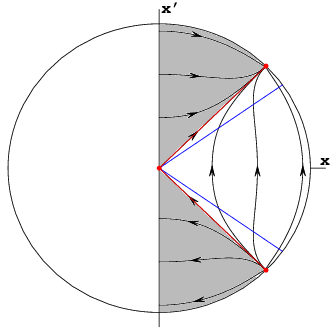
Figure 1: The phase portrait for $\Lambda=0$ and arbitrary $n$ in the case A type modifications. The shaded region is physically forbidden. The dark gray line (blue el.v.) denotes phase space location of $H^{2}=\infty$. The light gray line (red el.v.) which is a border of the physically allowed region, denotes phase space location of $H^{2}=0$. The zero energy level trajectories joining critical point at the finite domain with critical points at infinity divides the phase space in to two region occupied by the scalar field ($\alpha>0$) and the phantom scalar field ($\alpha<0$) trajectories. Only trajectories with $\alpha>0$ are physical and for all admissible initial conditions they tend to the final state of $H^{2}=0$ for $x=\infty$ ($p=\infty$ or $a=\infty$).

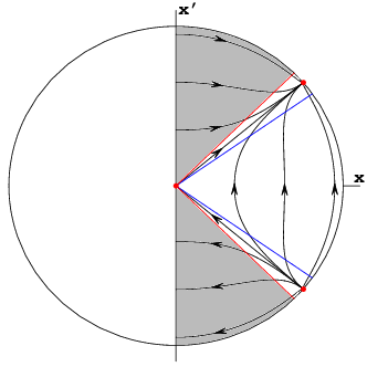
a) b)

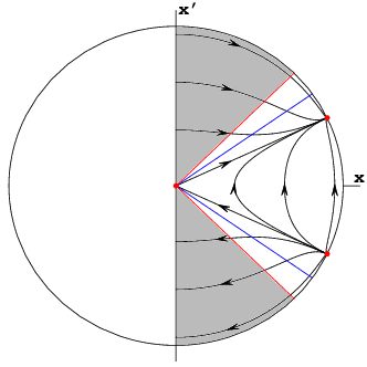
Figure 2: The phase portraits for $n=-1/2$ in the case A type modifications. a) For $0<\frac{\Lambda}{\Lambda_{0}}<\frac{3}{2}$ the scalar field ($\alpha>0$) and the phantom scalar field ($\alpha<0$) trajectories are physically allowed, but their evolution is different; the $\alpha>0$ trajectories start from anti de Sitter state and go through hyper-deflation state then bounce appears and next we have hyper-inflation state, the final state is de Sitter; the phantom trajectories for $x^{\prime}>0$ start from $H^{2}=0$ and tend to de Sitter state; b) For $\frac{3}{2}<\frac{\Lambda}{\Lambda_{0}}<3$ the situation is quite similar but the state of hyper-inflation (or hyper-deflation) appears only for phantom trajectories.

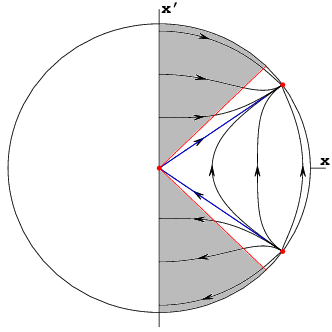
a) b)

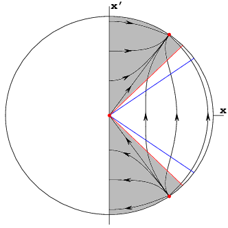
Figure 3: The phase portraits for $n=-1/2$ in the case A type modifications: a) For $\frac{\Lambda}{\Lambda_{0}}=\frac{3}{2}$ the trajectories with $\alpha>0$ after bounce tend to the critical state of $H^{2}=\infty$ for $x=\infty$, the phantom ($\alpha<0$) evolution for $x^{\prime}>0$ starts at $H^{2}=0$ state and tends to the same final state of $H^{2}=\infty$; b) For $\Lambda<0$ only the scalar field trajectories are physically allowed ($\alpha>0$), their evolution starts at $H^{2}=0$ and after hyper-deflation, bounce and hyper-inflation state ends at $H^{2}=0$.

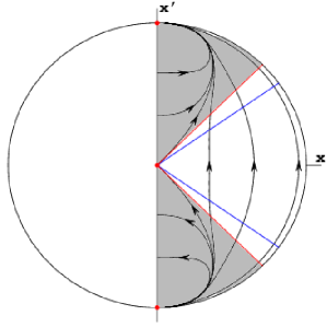
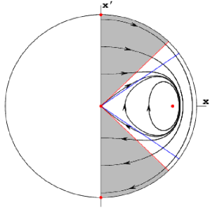
a) b) c) d)

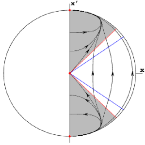
Figure 4: Phase portraits for a) $\Lambda>0$ and $n=0$; b) $\Lambda<0$ and $n=0$; c) $\Lambda>0$ and $n=-1/4$; d) $\Lambda<0$ and $n=-1/4$ in the case A type modifications. Note that the cases $n=0$ and $n=-1/4$ are topological equivalent.

III.2 Quadratic modifications from $\mathcal{O}(\mu^{4})$

The employ of the quadratic contribution from the $\mathcal{O}(\mu^{4})$ studied in the section II lead to the phenomenological Hamiltonian in the form

$$\mathcal{H}_{\text{phen}}=-\frac{3}{\kappa\gamma^{2}\bar{\mu}^{2}}\Big{(}\sin^{2}{(\bar{\mu}c)}+\frac{1}{3}\sin^{4}{(\bar{\mu}c)}\Big{)}+|p|^{3/2}\rho$$ (30)

where matter content is the same as in the previous case and is given by (21). In the same way like in the previous case we aim to calculate the effective Friedmann equation and then rewrite it in the point-like particle form. To achieve it we derive

$$\dot{p}=\left\{p,\mathcal{H}_{\text{phen}}\right\}=\frac{2\sqrt{|p|}}{\gamma\bar{\mu}}\sin{(\bar{\mu}c)}\cos{(\bar{\mu}c)}\big{(}1+\frac{2}{3}\sin^{2}{(\bar{\mu}c)}\big{)}$$ (31)

and with use of the Hamiltonian constraint we obtain the modified Friedmann equation

$$H^{2}=\frac{\kappa}{3}\rho\left(1+\frac{4}{3}\frac{\rho}{\rho_{\text{c}}}\right)\frac{5-3\sqrt{1+\frac{4}{3}\frac{\rho}{\rho_{\text{c}}}}}{1+\sqrt{1+\frac{4}{3}\frac{\rho}{\rho_{\text{c}}}}}.$$ (32)

Changing of variable $x=p^{1-n}$ we rewrite equation (32) to the form

$$\frac{\dot{x}^{2}}{2}\frac{1}{(1-n)^{2}}\frac{3}{\kappa\rho}\frac{1+\sqrt{1+\frac{4}{3}\frac{\rho}{\rho_{\text{c}}}}}{5-3\sqrt{1+\frac{4}{3}\frac{\rho}{\rho_{\text{c}}}}}-\frac{1}{2}x^{2}\Big{(}1+\frac{4}{3}\frac{\Lambda}{\Lambda_{0}}x^{\frac{1+2n}{1-n}}\Big{)}=2\frac{\alpha}{\Lambda_{0}}.$$ (33)

Performing the time transformation

$$\frac{d}{d\tau}=\sqrt{\frac{1}{(1-n)^{2}}\frac{3}{\kappa\rho}\frac{1+\sqrt{1+\frac{4}{3}\frac{\rho}{\rho_{\text{c}}}}}{5-3\sqrt{1+\frac{4}{3}\frac{\rho}{\rho_{\text{c}}}}}}\frac{d}{dt}$$ (34)

we obtain Hamiltonian of the point-like particle of the unit mass

$$\frac{1}{2}x^{\prime 2}+V(x)=E$$ (35)

where the potential function is given by

$$V(x)=-\frac{1}{2}x^{2}\Big{(}1+\frac{4}{3}\frac{\Lambda}{\Lambda_{0}}x^{\frac{1+2n}{1-n}}\Big{)}$$ (36)

and total energy

$$E=2\frac{\alpha}{\Lambda_{0}}.$$ (37)

Figs 5, 6, 7 and 8 represent the phase portraits for model with this type modification.

For this type of corrections the condition $\rho\geq 0$ corresponds to $x^{\prime 2}\geq x^{2}$. There is another condition for positivity of the Hubble function (32) and the time transformation (34) which is $\frac{5}{3}\geq\sqrt{1+\frac{4}{3}\frac{\rho}{\rho}_{c}}$. In the new variables $(x,x^{\prime})$ this is $x^{\prime 2}\leq\frac{25}{9}x^{2}$. The physical domain in the phase space for the type B corrections is defined by

$$x^{2}\leq x^{\prime 2}\leq\frac{25}{9}x^{2}.$$

This region is labelled as white on the phase portraits.

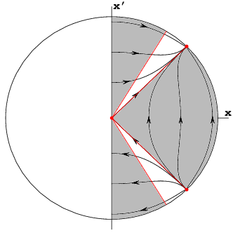
Figure 5: The phase portrait for $\Lambda=0$, arbitrary $n$ and the type B quadratic modifications. The shaded regions are physically not allowed. The borders of these regions denote the phase space location of the state $H^{2}=0$, only the scalar field ($\alpha>0$) trajectories are located in the physical domain. For $x^{\prime}>0$ they start from the state $H=0$ and tend to the final state of $H=0$ at $x=\infty$. The states $H=0$ represent the static Einstein universes which are reached asymptotically.

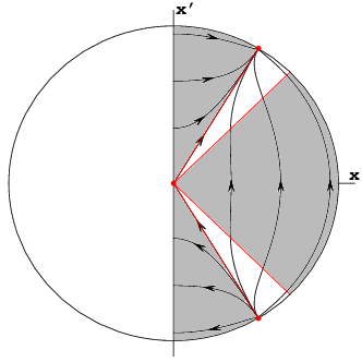
a) b)

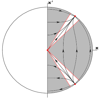
Figure 6: The phase portraits for $n=-1/2$ and the type B quadratic modifications: a) For $\frac{\Lambda}{\Lambda_{0}}=\frac{4}{3}$ only $\alpha<0$ trajectories are physical and for $x^{\prime}>0$ they start form the $H^{2}=0$ state for finite $x$ and go to $H^{2}=0$ for $x=\infty$; b) For $0<\frac{\Lambda}{\Lambda_{0}}<\frac{4}{3}$ both types of trajectories are allowed and they start form $H^{2}=0$ with finite $x$ and tend to the de Sitter state at infinity.

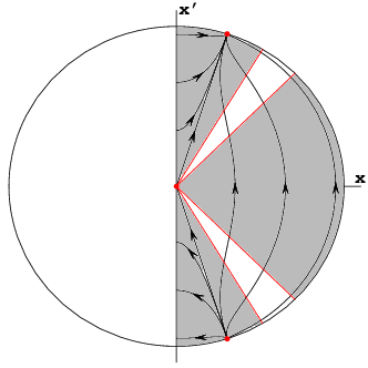
a) b)

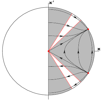
Figure 7: The phase portraits for $n=-1/2$ and the type B quadratic modifications from $\mathcal{O}(\mu^{4})$: a) $\frac{\Lambda}{\Lambda_{0}}>\frac{4}{3}$, b) $-\frac{3}{4}<\frac{\Lambda}{\Lambda_{0}}<0$.

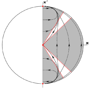
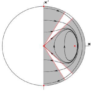
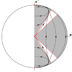
a) b) c) d)

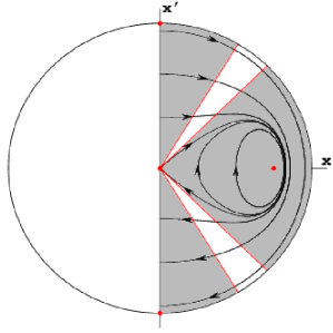
Figure 8: The phase portraits for model with the type B quadratic modifications for $n=0$: a) and b), $n=-1/4$: c) and d) and $\Lambda>0$: a) and c) (left panel), $\Lambda<0$: b) and d) (right panel). The physical trajectories lie in the domain labelled as white.

III.3 Exact solutions for the type A and B modifications

It is interesting that for both types of modifications we can find exact solutions for $x(\tau)$ or $p(\tau)$ for $n=-1/2$ and $n=0$. In the case of $n=-1/2$, $\alpha>0$ the modified Friedmann equation for the type A modification takes the form

$$\left(\frac{dx}{d\tau}\right)^{2}=-\frac{\alpha}{\Lambda_{0}}+x^{2}\left(1-\frac{1}{3}\frac{\Lambda}{\Lambda_{0}}\right).$$ (38)

The physical solutions of this equation correspond to the case

$$\frac{\Lambda}{\Lambda_{0}}<3.$$ (39)

Performing the direct integration of the equation (38) we obtain solution

$$x(\tau)=\sqrt{\frac{3\alpha}{3\Lambda_{0}-\Lambda}}\cosh\left[\sqrt{1-\frac{1}{3}\frac{\Lambda}{\Lambda_{0}}}(\tau-\tau_{0})\right]$$ (40)

or

$$p(\tau)=\left(\frac{3\alpha}{3\Lambda_{0}-\Lambda}\right)^{1/3}\cosh^{2/3}\left[\sqrt{1-\frac{1}{3}\frac{\Lambda}{\Lambda_{0}}}(\tau-\tau_{0})\right]$$ (41)

for the canonical variable.

In the case of $n=-1/2$, $\alpha<0$ (phantom) physical solutions are permitted for $\Lambda\in\mathbb{R}$. For $\Lambda/\Lambda_{0}<3$ we obtain

$$x(\tau)=\sqrt{\frac{-3\alpha}{3\Lambda_{0}-\Lambda}}\cosh\left[\sqrt{1-\frac{1}{3}\frac{\Lambda}{\Lambda_{0}}}(\tau-\tau_{0})\right],$$ (42)

for $\Lambda/\Lambda_{0}=3$ we obtain

$$x(\tau)=x_{0}+\sqrt{-\frac{\alpha}{\Lambda_{0}}}\tau,$$ (43)

for $\Lambda/\Lambda_{0}>3$ we obtain

$$x(\tau)=\sqrt{\frac{-3\alpha}{\Lambda-3\Lambda_{0}}}\sin\left[\sqrt{\frac{1}{3}\frac{\Lambda}{\Lambda_{0}}-1}(\tau-\tau_{0})\right].$$ (44)

Solutions for $p(\tau)$ are obtained taking $p(\tau)=x^{2/3}(\tau)$.

For $n=0$ the modified Friedmann equation takes the form

$$\left(\frac{dx}{d\tau}\right)^{2}=-\frac{\alpha}{\Lambda_{0}}+x^{2}-\frac{1}{3}\frac{\Lambda}{\Lambda_{0}}x^{3}.$$ (45)

The solution of this equation is expressed in terms of the Weierstrass $\wp$-function

$$x(\tau)=\frac{\Lambda_{0}}{\Lambda}\left[1-12\wp(\tau-\tau_{0};g_{2},g_{3})\right]$$ (46)

where

$$g_{2} = \frac{1}{12},$$ (47)

$$g_{3} = -\frac{1}{216}+\frac{1}{144}\left(\frac{\Lambda}{\Lambda_{0}}\right)^{2}\frac{\alpha}{\Lambda_{0}}.$$ (48)

For the $\Lambda<0,\alpha>0$ this solution represents a bouncing type of evolution. In the case $\Lambda>0,\alpha>0$ physical solutions are present when additional relation

$$\frac{4}{3}>\frac{\alpha}{\Lambda_{0}}\left(\frac{\Lambda}{\Lambda_{0}}\right)^{2}$$ (49)

is fulfilled and represents an oscillating type of evolution. In this case solutions for $x(\tau)$ and $p(\tau)$ are equal, $p(\tau)=x(\tau)$.

Analogous solutions for the type B modifications can be also obtained with the help of transformation $\Lambda\to-4\Lambda$ and $\alpha\to-4\alpha$ (see Table 1).

IV General properties of the phase portraits

The dynamical behaviour of the models considered is fully determined by the single potential function (27) or (36). Its diagram characterizes a type and location of the critical points of the dynamical system

$$\left\{\begin{array}[]{l}x^{\prime}=y\\ y^{\prime}=-\frac{\partial V}{\partial x}\end{array}\right.$$ (50)

System (50) is of the Newtonian type and at the finite domain of the phase space there can be only a saddle or a centre type critical points (or degenerated which are not interesting because we are only looking for generic cases). The type of a critical point is determined from the characteristic equation of the linearization matrix, namely

$$\lambda^{2}=-\frac{\partial^{2}V}{\partial x^{2}}\bigg{|}_{x_{0}},$$ (51)

calculated at the critical point. If $-\frac{\partial^{2}V}{\partial x^{2}}\big{|}_{x_{0}}>0$ eigenvalues are real of opposite signs and we have a saddle type critical point, and in case if $-\frac{\partial^{2}V}{\partial x^{2}}\big{|}_{x_{0}}<0$ eigenvalues are purely imaginary of opposite signs and a critical point is of a centre type.

Table 1: The Hamiltonian and derivative of the potential at the critical point for both types of corrections

	A	B
Hamiltonian	$\mathcal{H}_{A}=\frac{1}{2}x^{\prime 2}+V(x)=-\frac{1}{2}\frac{\alpha}{\Lambda_{0}}$	$\mathcal{H}_{B}=\frac{1}{2}x^{\prime 2}+V(x)=2\frac{\alpha}{\Lambda_{0}}$
potential	$V(x)=-\frac{1}{2}x^{2}\bigg{(}1-\frac{1}{3}\frac{\Lambda}{\Lambda_{0}}x^{\frac{1+2n}{1-n}}\bigg{)}$	$V(x)=-\frac{1}{2}x^{2}\bigg{(}1+\frac{4}{3}\frac{\Lambda}{\Lambda_{0}}x^{\frac{1+2n}{1-n}}\bigg{)}$
critical points :
arbitrary $n$	$x_{0}=0$, $\quad-\frac{\partial^{2}V}{\partial x^{2}}\Big{|}_{x_{0}}=1$	$x_{0}=0$, $\quad-\frac{\partial^{2}V}{\partial x^{2}}\Big{|}_{x_{0}}=1$
$-1/2<n\leq 0$	$x_{0}^{\frac{1+2n}{1-n}}=2(1-n)\frac{\Lambda_{0}}{\Lambda}$, $\Lambda>0$,	$x_{0}^{\frac{1+2n}{1-n}}=-\frac{1}{2}(1-n)\frac{\Lambda_{0}}{\Lambda}$, $\Lambda<0$,
	$-\frac{\partial^{2}V}{\partial x^{2}}\Big{|}_{x_{0}}=-\frac{1+2n}{1-n}$	$-\frac{\partial^{2}V}{\partial x^{2}}\Big{|}_{x_{0}}=-\frac{1+2n}{1-n}$

For the model with type A modifications (see also Table 1)

• $n=-1/2$, $x_{0}=0$: $\lambda=\pm\sqrt{1-\frac{1}{3}\frac{\Lambda}{\Lambda_{0}}}$

  a saddle for $\frac{\Lambda}{\Lambda_{0}}<3$

  a centre for $\frac{\Lambda}{\Lambda_{0}}>3$

• $-1/2<n\leq 0$:

  $x_{0}=0$ : $\lambda=\pm 1$ a saddle

  $x_{0}^{\frac{1+2n}{1-n}}=2(1-n)\frac{\Lambda_{0}}{\Lambda}$ and $\Lambda>0$: $\lambda=\pm i\sqrt{\frac{1+2n}{1-n}}$ a centre

For the model with type B modifications (see also Table 1)

• $n=-1/2$, $x_{0}=0$: $\lambda=\pm\sqrt{1+\frac{4}{3}\frac{\Lambda}{\Lambda_{0}}}$

  a saddle for $\frac{\Lambda}{\Lambda_{0}}>-\frac{3}{4}$

  a centre for $\frac{\Lambda}{\Lambda_{0}}<-\frac{3}{4}$

• $-1/2<n\leq 0$:

  $x_{0}=0$ : $\lambda=\pm 1$ a saddle

  $x_{0}^{\frac{1+2n}{1-n}}=-\frac{1}{2}(1-n)\frac{\Lambda_{0}}{\Lambda}$ and $\Lambda<0$: $\lambda=\pm i\sqrt{\frac{1+2n}{1-n}}$ a centre

Therefore all information about the critical points and their type contains the single potential function.

Figs 1–4 show representative cases of the global dynamics of the system of equations (29) and (27). Figs 5–8 show representative cases of the global dynamics for type B corrections.

We obtain different phase portraits for basic model parameters $(n,\Lambda)$, where $-1/2\leq n\leq 0$ and the cosmological constant belongs to the some characteristic intervals. For comparison we also present phase portraits for the case of the vanishing cosmological constant Fig. 1 for the case A and Fig. 5 for the B case. In the case A we can observe only critical point of a centre type located at the $x$ axis and critical point of a saddle type at the origin of the phase space (in principle at the origin a centre type critical point for $\Lambda/\Lambda_{0}>3$ can be present, but this case in not interesting because of it’s structural instability). Along the trajectories it is measured the new time variable which is a monotonic function of the original cosmological time but this flow can be incomplete, i.e., infinite cosmological time is mapped on the finite interval measured along the trajectory.

In the case of the positive cosmological constant and the case A modifications two characteristic evolutional scenarios are realized:

• A trajectory starts from the contracting deS_- stage and finishes at the expanding deS₊ stage. In the middle state the trajectory is undergoing the bounce in the vicinity of the intersection with the $p$-axis. In other words for such a evolution deS_- is the initial state and deS₊ is the final state (see Fig. 9).

• There is new non expected behaviour for the positive cosmological constant – emerging of oscillatory behaviour – without initial and final singularities and, in special case, without hyper-inflation and hyper-deflation states (see Fig. 10) for

  $$\alpha=\frac{\kappa}{6}p_{\phi}^{2}>\frac{1}{6}(1+2n)\Big{(}(1-n)\frac{\Lambda}{\Lambda_{0}}\Big{)}^{2\frac{1-n}{1+2n}}.$$

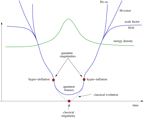
Figure 9: The schematic picture of the evolution with the positive $\Lambda$ for the monotonic models. The green curve represents the energy density. It is worth to note that this energy density is finite during whole evolution, even during transitions through singularities. The blue curve represents the schematic evolution of the scale factor for the investigated model. The dashed curve represents the classical evolution which is not realized in the presented quantum model.

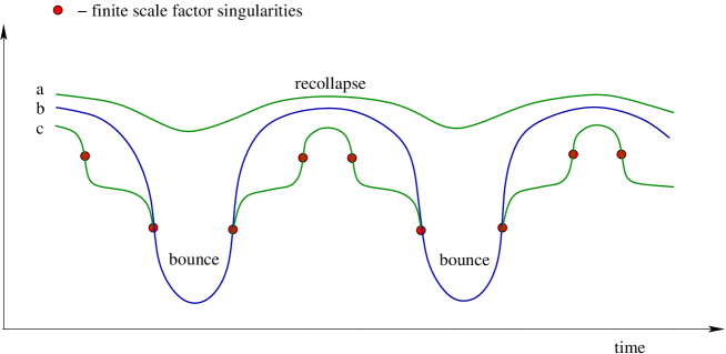
Figure 10: Generic evolutional scenarios for bouncing-oscillatory models with $\Lambda>0$ and the value of critical energy constant is $E_{\text{c}}=-\frac{1}{12}(1+2n)\Big{(}(1-n)\frac{\Lambda}{\Lambda_{0}}\Big{)}^{2\frac{1-n}{1+2n}}$: a) the oscillating model without the singularities $(E<E_{\text{c}})$; b) the oscillating model with double singularities at finite scale factor per period $(E=E_{\text{c}})$; c) the oscillating model with four singularities at the finite scale factor per period $(E>E_{\text{c}})$.

What it is interesting in these scenario is the universe is undergoing a phase of hyper-inflation in the vicinity of a singularity. This singularity is a curvature singularity at which the scale factor (as well as density) is finite but the Hubble function assumes infinite value. We mark a blue line in the phase portraits which shows the singularities reached by different trajectories. The algebraic equation for this line is independent of the value of the cosmological constant. But note that there are trajectories which do not intersect this line at all, they intersect it only at one point and at least they intersect it at two points. These three cases have been illustrated schematically in Fig. 10. If $E<E_{\text{c}}$ singularities are avoided.

The new evolutional scenario offered by the quantum correction is oscillating behaviour in universes with double singularities during the expansion (and contracting) period for the positive $\Lambda$. For other propositions of oscillatory models with bounce and phantom see Freese et al. (2008).

All emerging evolutional scenarios for the origin of the universe from the bounce are in principle testable because we have the Hubble function in respect of the redshift, which in order can be starting point for cosmography. In principle if the size of the universe is going to infinity there are three types of exits: $H$ is going to infinity, $H$ is approaching to the de Sitter state or $H$ is going to the zero. All these long term behaviour one can find in Fig. 9.

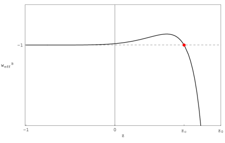
Figure 11: The dependence of the effective equation of state parameter on the redshift $z$ for both cases A (top) and B (bottom) of quantum corrections for $n=-1/2$ and $\Lambda>0$ (see phase portraits Fig. 2a and Fig. 6b). In both cases energy density approaches the cosmological constant $w_{\text{eff}}=-1$ case at the long time evolution. Top panel: in the type A correction the evolution begins at the bounce for the redshift value $z_{\text{b}}$, next the curvature singularity is present at $z_{\text{s}}$ and then $w_{\text{eff}}$ approaches the $-1$ value. Bottom panel: in the type B correction the evolution begins at $z_{0}$ when $H^{2}=0$, next the crossing of the phantom divide line is present at $z_{\text{c}}$ (marked as a dot) and then again $w_{\text{eff}}$ approaches $-1$.

The quantum corrections considered are dynamically equivalent to the effects of the decaying cosmological constant term with the effective equation of state coefficient parameterized by the scale factor or the redshift. This fictitious fluid which mimics dynamical effects of the quantum corrections can be calculated in the exact form for the both types of corrections. Using the general formulae

$$w_{\text{eff}}=-1-\frac{1}{3}\frac{d\ln{H^{2}}}{d\ln{a}}$$

and modified Friedmann equations (23) and (32) we obtain following forms of the equation of state parameter: for the type A correction

$$w^{A}_{eff}=-1+2\frac{\alpha a^{-6}}{\alpha a^{-6}+\frac{\Lambda}{3}}\bigg{[}\frac{1-\frac{2}{3}\frac{\rho}{\rho_{c}}}{1-\frac{\rho}{3\rho_{c}}}+\frac{\frac{\rho}{3\rho_{c}}}{\Big{(}1-\frac{2}{3}\frac{\rho}{\rho_{c}}\Big{)}\Big{(}\frac{3}{4}(1-\frac{2}{3}\frac{\rho}{\rho_{c}})^{2}+\frac{1}{4}\Big{)}}\bigg{]}$$ (52)

and for the type B correction

$$w^{B}_{eff}=-1+2\frac{\alpha a^{-6}}{\alpha a^{-6}+\frac{\Lambda}{3}}\bigg{[}\frac{1+\frac{8}{3}\frac{\rho}{\rho_{c}}}{1+\frac{4}{3}\frac{\rho}{\rho_{c}}}-\frac{\frac{16}{3}\frac{\rho}{\rho_{c}}}{\Big{(}5-3\sqrt{1+\frac{4}{3}\frac{\rho}{\rho_{c}}}\Big{)}\Big{(}1+\sqrt{1+\frac{4}{3}\frac{\rho}{\rho_{c}}}\Big{)}\sqrt{1+\frac{4}{3}\frac{\rho}{\rho_{c}}}}\bigg{]}$$ (53)

where

$$\frac{\rho}{\rho_{c}}=\frac{3}{\Lambda_{0}}a^{2(2n+1)}\Big{(}\alpha a^{-6}+\frac{\Lambda}{3}\Big{)}.$$ (54)

Equation (54) gives us opportunity to calculate the redshift distance to the characteristic moments of the universe evolution. For the type A correction the bounce occurs when $\rho/\rho_{c}=3$ and using (54) we have that at the scale factor value fulfilling relation

$$a^{2(2n+1)}\Big{(}\frac{\alpha}{\Lambda_{0}}a^{-6}+\frac{1}{3}\frac{\Lambda}{\Lambda_{0}}\Big{)}=1$$

the bounce is present. In the special case of $n=-1/2$, the value of the redshift at the bounce is

$$z_{\text{b}}=-1+\sqrt[6]{\frac{\Lambda_{0}}{\alpha}\Big{(}1-\frac{1}{3}\frac{\Lambda}{\Lambda_{0}}\Big{)}}.$$ (55)

Another characteristic moment of the model evolution is the curvature singularity appearing at the redshift (for $n=-1/2$)

$$z_{s}=-1+\sqrt[6]{\frac{\Lambda_{0}}{\alpha}\Big{(}\frac{1}{2}-\frac{1}{3}\frac{\Lambda}{\Lambda_{0}}\Big{)}}.$$ (56)

For the type B corrections evolution begins when $\rho/\rho_{c}=4/3$, that is, for $n=-1/2$ at

$$z_{0}=-1+\sqrt[6]{\frac{1}{3}\frac{\Lambda_{0}}{\alpha}\Big{(}\frac{4}{3}-\frac{\Lambda}{\Lambda_{0}}\Big{)}}$$ (57)

There is another important moment in the evolution appearing only for the type B correction, namely the crossing of the phantom divide line (Fig. 11 bottom). In this case the during the evolution of the universe $w_{\text{eff}}$ starts from a large negative value, crosses the line $w_{\text{eff}}=-1$, then reaches the maximum and now decreases to asymptotically to minus one. Solving Eq. (53) for $w^{B}_{\text{eff}}=-1$ we find that $\rho/\rho_{c}=\frac{1}{8}(1+2\sqrt{6})$ and for $n=-1/2$ at the redshift value

$$z_{\text{c}}=-1+\sqrt[6]{\frac{1}{3}\frac{\Lambda_{0}}{\alpha}\Big{(}\frac{1}{8}(1+2\sqrt{6})-\frac{\Lambda}{\Lambda_{0}}\Big{)}}$$ (58)

the crossing of the phantom divide line happens.

V Conclusions

In this paper we have considered the influence of the modifications to the field strength expression for the effective dynamics in the loop quantum cosmology. We have studied the sensitivity of evolutional scenarios on the choice of model parameters $(n,\Lambda)$. For the classification of evolutional paths in arising the loop quantum cosmology models it is natural to adopt the dynamical systems methods which offers full classification of dynamical outcome for all admissible initial conditions. We consider two types of quantum modifications labelled as modification (A) $\mathcal{O}(\mu^{4})$ and the quadratic modifications from $\mathcal{O}(\mu^{4})$ (B) (for details see Section II).

From mathematical point of view the dynamics is represented by $2D$ dynamical system of the Newtonian type. From the cosmological point of view quantum corrections are manifested by decaying part of the cosmological constant $\Lambda$ term. Main advantage of using dynamical systems methods lies in the possibility of studding complexity of dynamics. In the geometric language of the phase space we can analyze the asymptotic stability of the solutions. From this analysis we obtain that a generic feature of dynamics is emergence of the bounce instead of the initial singularity. We can find easily beginning and final states of dynamics in its long time behaviour using the phase space compactification with the circle at infinity. For the positive cosmological constant and (A) type corrections, in principle, there are three types of outcomes (and incomes respectively because the dynamics is invariant under the reflection symmetry $\dot{p}\to-\dot{p}$), namely the expanding de Sitter state deS₊, $H=\infty$ state or the Einstein static universe $H=0$.

The new feature of dynamics within models with (A) type corrections is appearance of singularities at the finite scale factor and the super-accelerating phase of expansion in the vicinity of this singularity. However, we demonstrate that this singularity can be avoided for some choice of the critical value of total energy $E_{\text{c}}$.

Another new phenomenon is the emergence of oscillating models for positive value of the cosmological constant with single or double curvature singularities for the finite scale factor. We demonstrate that the dynamics with (A) and (B) a type of corrections are dual and after the transformations $\Lambda\to-4\Lambda$ and $\alpha\to-4\alpha$ one can obtain the evolution of models with the massless scalar field from evolution of the phantom scalar field (formally this means that we consider a opposite sign of total energy and the cosmological constant). The main difference between the models with positive and negative cosmological constant is that in the latter case incomes and outcomes always represents the static Einstein Universe.