Orbital current patterns in doped two-leg $Cu$-$O$ Hubbard ladders

Abstract

In the weak coupling limit, we investigate two-leg ladders with a unit cell containing both $Cu$ and $O$ atoms, as a function of doping. For purely repulsive interactions, using bosonization, we find significant differences with the single orbital case: a completely massless quantum critical regime is obtained for a finite range of carrier concentration. In a broad region of the phase diagram the ground state consists of a pattern of orbital currents plus a density wave. NMR properties of the $Cu$ and $O$ nuclei are presented for the various phases.

I Introduction

Over the past two decades, the description of strongly correlated electron materials has been one of the most actively pursued problems in condensed matter physics. When the strength of Coulomb interactions between carriers is of the order of (or larger than) their kinetic energy, many new remarkable phenomena may occur. Their fingerprints are seen in experiments done on systems such as cuprate compounds with high temperature superconductivity[1] , cobaltites with large termopower[2], magnesium oxides with colossal magnetoresistance[3], or heavy fermions[4]. Among these materials, cuprates play a special role. At half filling they are insulators with antiferromagnetic (AF) order, but, with doping, a sequence of phases is observed including spin-glass, pseudogap, d-type superconductivity (SCd) and eventually Fermi-like behavior for very large carrier concentrations.

Unfortunately there is, to date, no consensus on a theoretical model that would allow one to describe the physics of the $Cu$-$O$ planes. In order to get insight into this strong correlation problem, the study of ladder structures [5, 6] has proven quite useful. Ladders are the simplest systems that interpolate between one- and two- dimension. They constitute the quasi- one dimensional analog of the $Cu$-$O$ sheets and, because of the reduced dimensionality, even weak interactions lead to dramatic effects. In the one dimensional (1D) case, the weak- and strong- interaction limits are usually smoothly connected [7]. Controlled non-perturbative methods – like bosonization or conformal field theory – and numerical techniques can be used to analyse these systems.

Compounds characterized by a ladder structure [5, 6], such as SrCuO, have been synthesized. They show a variety of unusual properties, for example large magnetic fluctuations, SCd with purely repulsive interactions and metal-insulator transitions under high pressure [8, 9, 10, 11, 12]. For these materials, increasing the pressure amounts to changing the bandwidth, and hence the ratio of Coulomb to kinetic energies in the ladder structure.

These experimental developments provided a strong incentive for theorists to study two-leg ladders with Hubbard interactions between electrons. In the weakly interacting limit, renormalization group (RG) analysis [13] was used to explore their phase diagram[14, 15, 16, 17, 18, 19, 20]. Tsuchiizu and Suzumura [21], and Tsuchiizu and Furusaki [22] performed an RG analysis in bosonization language in order to explore the regime of dopings close to half filling. Using current algebra, where spin rotational symmetry was introduced a priori in order to derive RG equations, Balents and Fisher [19, 20] established the phase diagram of two leg ladder versus doping, showing that there was interesting physics at finite dopings. They identified a sequence of phases, labelled $CnSm$ with $n$ (m) gapless charge (spin) modes. Numerical DMRG calculations focused on the large U limit [23, 24, 25], the so called t-J approximation at half filling [26, 27, 28]. The relevance of interchain hoppings on the low energy physics was also adressed [29, 30, 31, 32].

The above mentioned papers all assume that, in the low energy limit, the $Cu$-$O$ system can be reduced to an effective single orbital model. In the context of two dimensional (2D) cuprate materials, such reduction to a single orbital model was proposed by Zhang and Rice[33] and it allowed one to derive phase diagrams for these systems [34, 1]. However this simplification was called into question, and it was pointed out that it is necessary to retain the full three band nature of the model in order to capture the important physics [35, 36]. This issue becomes particularly relevant when one examines the possible existence of orbital current phases. Such phases were initially proposed for the Hubbard model [37]. They were subsequently analyzed by various authors [38, 39, 40, 1], but in slave boson and in numerical calculations one finds that they are unstable. For single band ladder models, controlled calculations appropriate to 1D reveal that for special choices of interactions – which must include non local terms – staggered flux patterns are stable. This phase breaks the translational symmetry of the lattice [41, 42]. According to some authors [43, 1], the 2D version of this state (the DDW phase) describes the pseudogap phase of the cuprates. An alternative type of orbital current pattern, which preserves the lattice translational symmetry, was advocated to describe the pseudogap phase [35, 36]. It then requires using a three band model. Recent experimental data taken from neutron measurements[44] and polar Kerr effect[45] would be consistent with the latter proposal, but more studies are clearly needed to fully corroborate this scenario.

Motivated by these considerations, Lee, Marston and Fjarestad [46] (see also Ref. 47) generalized the system of RG equations written in current algebra language by Balents and Fisher to study the $Cu$-$O$ Hubbard ladder. Their work was however limited to the half-filled case, where umklapp terms dominate the physics, giving rise to Mott transitions. In a recent rapid communication[48] we outlined the method which allowed us to map out the full diagram of the $Cu$-$O$ ladder as a function of doping.

The aim of the present paper is to provide details of our derivation, and to present new results which are experimentally testable. In our work, oxygen atoms are taken into account at each calculation step, which allows us to probe their influence. First, they lead to new types of phases compared with the single orbital case: a Luttinger liquid (LL) regime is found for a fine range of dopings and, in a broad region of the phase diagram, the ground state displays an orbital current pattern plus density wave quasi long-range order. Our study thus underscores the importance of including these additional degrees of freedom in the structure, in particular with regards to the existence and to the stability of currents patterns. Although our results have been derived for the specific case of ladders, they have potential relevance to the physics of 2D cuprate materials as well. Second, spectroscopic tools measuring local properties, such as NMR, are predicted to give different signatures depending on wether they probe Cu or O sites. In the large U limit, for 2D cuprates, it is believed that spin fluctuations on oxygen sites merely track those on the copper sites[34]. The advantage of revisiting the issue in a quasi-1D context is that one can monitor spin excitations on oxygen atoms both in the small and large U limits using bosonization techniques. This is done in the present paper for various dopings in the small U limit; we do find differences between the NMR signal on the copper and oxygen atoms at low temperature, when gaps set in, but not at higher temperature in the Luttinger liquid (LL) regime.

The paper is organized as follows: in Sec. II we define the model including the interactions relevant to the low energy physics. In the continuum limit the quadratic part of the Hamiltonian is diagonal in a particular basis, $B_{o}$. We give the relations between this basis, the bonding/antibonding basis $B_{o/\pi}$ (relevant in the non-interacting case) and the total/transverse density basis $B_{+-}$ (the most appropriate to write ”backward” interactions).

In section III we present a new method which allows one to set up the RG equations in the case of generic doping. [48]. One of its salient features is that it treats the rotation of $B_{o}$ with respect to $B_{+-}$ during the flow. This effect needs to be taken into account in order to perform all calculations properly. We list the resulting set of equations; their derivation is presented in the Appendix.

The various flows and the resulting phase diagram are given in section IV. First we assess the impact of the additional degrees of freedom, hence we set all Coulomb interactions pertaining to the $O$ atoms and direct interoxygen hoppings to zero. Some of the results obtained in previous work[19] can now be checked using our improved RG method. In constrast with the single orbital case, we find an intermediate doping range where all spin and gap modes are massless (i.e a quantum critical line). Next, interactions involving oxygen atoms and hoppings between these atoms are introduced. We find that interoxygen hoppings promote a phase of orbital currents and we analyze its structure. Spin-rotational symmetry was not imposed a priori, but we checked that the required property was preserved during the flow. This provides a check on the consistency of our calculations. In the case of massive regimes the evolution of the gaps with doping is shown. We briefly examine the impact of umklapp terms which are present at half filling.

In section V, we compute spin correlation functions, which allows us to derive the Knight shifts K and the relaxation rates $T_{1}$ for Cu and O nuclei. There are several improved features in our work. In Ref. 21, spin-spin correlation functions were calculated in the low temperature limit, using Majorana pseudo-fermions for the spin part; this assumes that gap opening in the spin and in the charge modes occur at well separated $T$. In bosonization language, spin-spin correlation function are easily obtained in all cases. For instance, if one treats spin and charge density fluctuations on equal footing, one shows that the uniform part of the susceptibility approaches a quantum critical point as doping increases and that, at low temperatures in the gapped phase, the staggered part gives a different temperature dependence for each atom in the elementary cell. We also discuss physical implications of the orbital current phase.

II The model

II.1 Hubbard Hamiltonian for $Cu-O$ two-leg ladders

We consider a two-leg ladder with a unit cell containing two $Cu$ and five $O$ atoms. Two edge oxygen sites are included because they would provide connections with neighboring ladders (which are not considered in the present work).

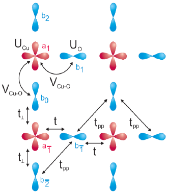
Figure 1: Energy contributions to the hamiltonian of the $Cu$-$O$ Hubbard ladder; the figure shows two-unit cells. Subscripts in the $a$, $b$ annihilation operators track the coordinate of the various atoms in a cell.

The hamiltonian of this system is divided in two parts: the kinetic energy of electrons moving on the lattice $H_{T}$ and electron interactions $H_{int}$

$$H=H_{T}+H_{int}$$ (1)

The explicit form of the first, tight-binding, part is

$$H_{T}=\sum_{j\sigma}(\sum_{m\in Cu}\epsilon_{Cu}n_{mj\sigma}+\sum_{m\in O}\epsilon_{O}n_{mj\sigma}-\sum_{m\in Cu}t[a_{mj\sigma}^{{\dagger}}(b_{mj\sigma}+b_{mj-1,\sigma})+\text{H.c.}]\\ -\sum_{m\in Cu}t_{\bot}[a_{mj\sigma}^{{\dagger}}(b_{m+1,j\sigma}+b_{m-1,j\sigma})+\text{H.c.}])-\sum_{m=\in O(leg)}t_{pp}[b_{mj\sigma}^{{\dagger}}(b_{m+1,j\sigma}+b_{m-1,j\sigma}+b_{m+1,j-1\sigma}+b_{m-1,j-1\sigma})+\text{H.c.}])$$ (2)

where $a_{mj\sigma}(b_{mj\sigma})$ annihilates holes with spin $\sigma$ on a copper (oxygen) site, $j$ labels cells along the chain and $m$ labels the atoms within each cell. $n_{mj\sigma}=a_{mj\sigma}^{{\dagger}}a_{mj\sigma}$ is the density of particles on site $m$, and we use here hole notation such that $t$, $t_{\bot}$, $t_{pp}$ are all positive. $\epsilon=\epsilon_{O}-\epsilon_{Cu}$ is the difference between the oxygen and copper on-site energies.

LDA determined values [49] of the parameters pertaining to SrCuO systems show that interladder hopping amplitudes are at least one order of magnitude smaller than their intraladder counterparts, so that the two-leg ladder description is an excellent starting point for these compounds. Inside the elementary cell, $t$ and $t_{\bot}$ are the dominant hoppings and their values are comparable. The difference between the electronic $Cu$- $d$ and $O$- $p$ state energies $E_{Cu}$ and $E_{O}$, is about 0.5t. There does not appear to be ab initio determinations of Coulomb terms for SrCuO ladders, but from what is known for cuprates, we may estimate a local $U$ of order $5t$ for the $Cu$ sites, meaning a strongly interacting regime. In the following we will use constant values of the band parameters $t=t_{\perp}=1$ and $\epsilon=0.5$, and treat the other observables ($U_{Cu}$, $t_{pp}/t$, $U_{O}/U_{Cu}$, $V_{Cu-O}/U_{Cu}$) as tunable variables. In order to gain insight into the physics of the multiband case, we analyze the above model using a renormalization group procedure in the interactions, i.e we assume that all of these are smaller than the kinetic energy; hence, the validity of the solutions cannot be ascertained, in the event when some of the interactions were to grow so large during the flow that they became of the order of the bandwidth. As was stated above, the experimental regime corresponds to a situation where Coulomb terms are sizable. Nevertheless the RG approach allows one to obtain a full analytical solution of this complicated problem, and to make detailed comparisons with the physics of the one band system. Furthermore, for the case of the single band ladder one finds that the physical properties in the weakly- and strongly- interacting limits are smoothly connected. We will come back to that point when we discuss our results.

Eigenvalues and eigenvectors of the non-interacting part are simply obtained by Fourier transforming $H_{T}$. Since $\epsilon$ is of order $t$, we neglect the non-bonding and antibonding higher energy bands which are mostly of $p$-type character, and this reduces the model to two lowest lying bands crossing the Fermi energy. The Hamiltonian is:

$$H_{T}=\sum_{k\alpha\sigma}e_{\alpha}(k)n_{k\alpha\sigma}$$ (3)

where $\alpha=0,\pi$ denotes the bands and $\sigma$ are spin indices. The operators corresponding to the eigenstates of $H_{T}$ are

$$a_{mk\sigma}\;\;(\textrm{or}\;\;b_{mk\sigma})=\sum_{\alpha}\lambda_{m\alpha}a_{\alpha k\sigma}$$ (4)

$e_{\alpha}(k)$ are the eigenvalues of $H_{T}$ (the $Cu$-$O$ distance is set to unity), and $\lambda_{m\alpha}$ are the amplitudes of the overlaps of the eigenvectors with the atomic wavefunctions in the unit cell. This defines the bonding ($o$) and antibonding ($\pi$) eigenbasis $B_{o/\pi}$. For $t_{pp}\neq 0$, the $o$ and $\pi$ energy bands are the two lowest, real solutions of the characteristic equation

$$\begin{split}(\epsilon-e_{o}(k))(3t_{\perp}^{2}+\epsilon^{2}-e_{o}(k)^{2})-2(1+\cos(k))(-6t_{pp}t_{\perp}t-t^{2}(\epsilon-e_{o}(k))+3t_{pp}^{2}(\epsilon+e_{o}(k)))=0\\ (\epsilon-e_{\pi}(k))(t_{\perp}^{2}+\epsilon^{2}-e_{\pi}(k)^{2})-2(1+\cos(k))(-2t_{pp}t_{\perp}t-t^{2}(\epsilon-e_{\pi}(k))+t_{pp}^{2}(\epsilon+e_{\pi}(k)))=0\\ e_{n}=\epsilon\end{split}$$ (5)

Including $t_{pp}$ increases the values of the $\lambda_{bi\alpha}$ for the $O$ atoms and makes the $o$ and $\pi$ bands more asymmetric, but there are still only two bands crossing the Fermi energy, so that the analysis remains valid. We note, however, that the contribution of the oxygen $p$-orbital perpendicular to the one participating in the $Cu$-$O$ bonding increases as $t_{pp}$ grows larger, until, for $t_{pp}>0.5t$, it dominates that of the copper d-orbital. Hence, we confine the range of variation of $t_{pp}$ to $0$-$0.5t$.

The interaction part in fermionic language is given by:

$$H_{int}=\sum_{j}(\sum_{m\in Cu}U_{Cu}n_{mj\uparrow}n_{mj\downarrow}+\sum_{m\in O}U_{O}n_{mj\uparrow}n_{mj\downarrow}+\sum_{m\in Cu,n\in O}\sum_{\sigma,\sigma^{\prime}}V_{Cu-O}n_{mj\sigma}n_{nj\sigma^{\prime}})$$ (6)

II.2 The continuum limit and bosonization

We now express the Hamiltonian in bosonic representation. The procedure is standard [7, 50] and we only outline the main steps here. We linearize the dispersion relation in the vicinity of the Fermi energy:

$$H_{T}=\sum_{|q|<Q}\sum_{r\alpha\sigma}rqV_{F\alpha}a^{{\dagger}}_{\alpha rq\sigma}a_{\alpha rq\sigma}$$ (7)

$r=\pm 1$ denotes right and left movers, with momenta close to their respective $\pm k_{F}$, $Q$ is a momentum cutoff. The boson phase fields denoted by $\phi_{\sigma\alpha}(x)$ are introduced for each fermion specie. $\sigma\alpha$ contains spin and band indices, x is the spatial coordinate along the ladder. Fermionic operators are expressed in term of the bosonic field $\phi_{\sigma\alpha}(x)$ and $\theta_{\sigma\alpha}(x)$ related to carriers fluctuations, by

$$\psi_{r\sigma\alpha}\simeq\eta_{r\sigma\alpha}\exp(\imath k_{F\alpha})\exp(\imath(r\phi_{\sigma\alpha}-\theta_{\sigma\alpha}))$$ (8)

where $\eta_{\sigma\alpha}$ are the Klein factors which satisfy the required anticommutation relations for fermions. These $\eta_{\sigma\alpha}$ do not contain any spatial dependence and they commute with the Hamiltonian operator. They only influence the form of the order operator in bosonic language (through terms of the form $\eta_{\sigma\alpha}\eta_{\sigma\alpha^{\prime}}$) and the signs of the non-linear couplings through a $\Gamma$ coefficient (the eigenvalue of the $\eta_{\sigma\alpha}\eta_{\sigma\alpha^{\prime}}\eta_{\sigma\alpha^{\prime\prime}}\eta_{\sigma\alpha^{\prime\prime\prime}}$ operator). The operator is unitary so $\Gamma^{2}=1$. This equality applies also to linear combinations of fields (change of basis); Following Ref. 22, we choose $\Gamma=+1$ in the $\sigma+/-$ basis (see below). We also introduce the phase field $\theta_{\sigma\alpha}(x)$; its spatial derivative $\Pi_{\sigma\alpha}(x)=\partial_{x}\theta_{\sigma\alpha}(x)$ is canonically conjugated to $\phi_{\sigma\alpha}(x)$.

Now the hamiltonian may be rewritten using the above phase fields. The interaction term in the Hamiltonian can be split in two parts; one part only depends on the density of right and left movers, and gives – as does the kinetic energy – a contribution quadratic in the fields $\phi_{\nu}$ and $\theta_{\nu}$, (where $\nu$ labels the eigenmodes in the diagonal basis) of the form

$$H_{0}=\sum_{\nu}\int\frac{dx}{2\pi}[(u_{\nu}K_{\nu})(\pi\Pi_{\nu})^{2}+(\frac{u_{\nu}}{K_{\nu}})(\partial_{x}\phi_{\nu})^{2}]$$ (9)

For the non-interacting system, one has $K_{\nu}=1$ for all modes, and $H_{0}$ is quadratic in the diagonal density basis which is simply $B_{o\pi}$ (the momentum $k_{\perp}$ associated with the rungs is either 0 or $\pi$). Another basis commonly used in the literature is the total/transverse one $B_{+-}$. It is related to $B_{o\pi}$ by:

$$\phi_{\mu+(-)}=\frac{\phi_{\mu o}\pm\phi_{\mu\pi}}{\sqrt{2}}$$ (10)

where $\mu$ stands for spin or charge depending on which density is considered.

In general $\hat{K}$ in (9) is a matrix, the form of which depends on the basis in which the densities are expressed. For example if we use $B_{o\pi}$ at the start of the calculation (the basis which diagonalizes the tight-binding part of the Hamiltonian), we obtain

$$\hat{u}\cdot\hat{K}^{-1}=\left(\begin{array}[]{cccc}V_{Fo}&g_{0\pi}^{\parallel}&g_{00}^{\perp}&g_{0\pi}^{\perp}\\ g_{0\pi}^{\parallel}&V_{F\pi}&g_{0\pi}^{\perp}&g_{\pi\pi}^{\perp}\\ g_{00}^{\perp}&g_{0\pi}^{\perp}&V_{Fo}&g_{0\pi}^{\parallel}\\ g_{0\pi}^{\perp}&g_{\pi\pi}^{\perp}&g_{0\pi}^{\parallel}&V_{F\pi}\\ \end{array}\right)$$ (11)

and

$$\hat{u}\cdot\hat{K}=\left(\begin{array}[]{cccc}V_{Fo}&0&0&0\\ 0&V_{F\pi}&0&0\\ 0&0&V_{Fo}&0\\ 0&0&0&V_{F\pi}\\ \end{array}\right)$$ (12)

where $V_{Fo/\pi}$ are the Fermi velocities in the $o$ and $\pi$ bands and $g_{ij}^{\perp(\parallel)}$ are interactions between electron densities in the $i$ and $j$ bands, with perpendicular (parallel) spin.

In order to express the hamiltonian in a Gaussian form (Eq. 9), which is quite convenient for the RG calculation, we diagonalize $\hat{K}$. This defines the $B_{o}$ basis. In general, $B_{o}$ is neither the bonding/antibonding basis $B_{o\pi}$, nor the total/transverse basis $B_{+-}$. We define the S matrix which describes the relative orientation of the $B_{o}$ and $B_{+-}$ bases:

$$S=\frac{\sqrt{2}}{2}\left(\begin{array}[]{cccc}P_{1}&Q_{1}&0&0\\ -Q_{1}&P_{1}&0&0\\ 0&0&P_{2}&Q_{2}\\ 0&0&-Q_{2}&P_{2}\\ \end{array}\right)$$ (13)

One can express the parameters $P_{i}$ and $Q_{i}$ with the help of angles $\alpha$ (for the spin part) and $\beta$ (for the charge part):

$$\begin{split}P_{1}&=\cos\alpha+\sin\alpha\\ Q_{1}&=\cos\alpha-\sin\alpha\\ P_{2}&=\cos\beta+\sin\beta\\ Q_{2}&=\cos\beta-\sin\beta\end{split}$$ (14)

The remaining part of the interactions has a non-linear, cosine, form, in bosonization language. The most convenient basis to express this contribution is $B_{+-}$ and one finds[7, 50]

$$H^{NL}_{int(1)}=-g_{1c}\int dr\cos(2\phi_{s+})\cdot\cos(2\theta_{c-})+g_{1a}\int dr\cos(2(\phi_{s+})\cdot\cos(2(\theta_{s-})-g_{2c}\int dr\cos(2(\theta_{c-})\cdot\cos(2(\phi_{s-})+\\ +g_{4a}\int dr\cos(2\phi_{s-})\cdot\cos(2\theta_{s-})+g_{1}\int dr\cos(2\phi_{s+})\cdot\cos(2\phi_{s-})+g_{2}\int dr\sin(2\phi_{s-})\sin(2\phi_{s+})+g_{\parallel c}\int dr\cos(2\theta_{c-})\cdot\cos(2\theta_{s-})$$ (15)

where $\Gamma$ coefficients determine the signs of the $g_{i}$ couplings (for instance, this gives minus signs for $g_{1c}$ and $g_{2c}$). We use the following notation: indices 1 to 4 refer to the standard g-ology processes for the left and right moving carriers, letters $a$ to $d$ correspond to similar processes, when the $o$ and $\pi$ bands labels are used instead of the left or right labels. The relation between the $g_{i}$ couplings and the ones in (6) is given in Appendix A. Note that in the quadratic piece, both $g_{2}$ and $g_{4}$ -type terms need to be included, in order to properly account for magnetic fluctuations[51]. Examples of interaction processes are shown in Fig. 2.

Figure 2: Diagram showing some of the scattering processes. Blue (green) lines are for carriers in the $o(\pi)$ bands. This illustrates the notation used for the cosine-type terms

For instance, the two $g_{1d}$ terms describe events where one right- and one left- moving fermion, both belonging to the same ($0$ or $\pi$) band, backscatter within that band. If we bosonize this contribution, we find two terms, $g_{1d}\cos(\phi_{1}+\phi_{2})$ and $g_{1d^{\prime}}\cos(\phi_{1}-\phi_{2})$, instead of $g_{1(2)}$. $g_{1}$ and $g_{2}$ correspond to the sum and to the difference of these “1d”-type processes respectively ($g_{1}=\frac{g_{1d}+g_{1d^{\prime}}}{2}$, $g_{2}=\frac{g_{1d^{\prime}}-g_{1d}}{2}$), and $g_{2}\neq 0$ when the $O$ atoms are included. If the two bands were equivalent only the $g_{1}$ process would be present.

In a standard Hubbard model, only spin perpendicular terms are present at bare level, and the last term in Eq. (15) does not appear at the beginning of the flow. However, Bourbonnais pointed out [52] that, during the flow towards the fixed point, additional scatterings involving electrons with parallel spins are generated by the RG procedure. In our case, we are including a $V_{Cu-O}$ term so that, right from the start, our model contains interactions between carriers with parallel spin. $V_{Cu-O}$ gives rise to a non-linear cosine term while the other spin-parallel processes, which are generated by the RG procedure, give contributions to the various $K$.

The $g_{4a}$ term has a non-zero conformal spin and generates two extra couplings during the renormalization:

$$H^{NL}_{int(2)}=-G_{p}\int dr\cos(4\phi_{s-})-G_{t}\int dr\cos(4\theta_{s-})$$ (16)

These additional terms need to be taken into account, because they might become relevant when the other interactions scale to zero.

III The Renormalization Group analysis

III.1 Incommensurate filling

We start from the quadratic part of the Hamiltonian, and treat the non-quadratic part (15) in perturbation, using a renormalization group procedure. We compute the corrections to the correlation functions to second order in $g$, and we incorporate them into the LL parameters $K$. However $g$ terms are expressed in the $B_{+-}$ basis while the quadratic part (9) is diagonal in the $B_{o}$ basis, so the $P_{i}(\alpha,\beta)$ and $Q_{i}(\alpha,\beta)$ coefficients come into play. As a result, off-diagonal terms are generated in the $K$ matrix during the RG iteration. At this stage, $B_{o}$ is no longer the diagonal basis. In order to fix this, the $B_{o}$ basis has to rotate during a renormalization cycle. In addition to the standard RG equations for the interactions, we need to find the RG flow of the angles $\alpha$ (for the spin density basis rotation) and $\beta$ (for the charge density basis rotation). So, first we determine the corrections $dK_{1}$,…,$dK_{4}$, $dB_{12}$, $dB_{34}$ that change the entries of the $K$ matrix during the intial RG phase. Next, we go back to $B_{+-}$, using the transformation $S^{-1}$; Since $B_{+-}$ is a fixed basis, the increments of the $K$ matrix elements give the RG step corrections expressed in the $B_{+-}$ basis. This new matrix is diagonalized by the operator $S(\alpha+d\alpha,\beta+d\beta)$ where the angles $d\alpha$, $d\beta$ depend on $dB_{\mu-\mu+}$ and $dK_{\mu-(\mu+)}$ ($\mu=c,s$). The procedure is summarized in the diagram shown in Fig. 3.

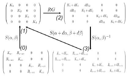
Figure 3: Diagram showing the flow of the diagonal basis during the renormalization. The bottom row, shows the matrix in the fixed $B_{+-}$; the top row corresponds to the diagonal basis, used to write down the RG equations.

A detailed derivation is given in Appendix B where, for the incommensurate case, we set all umklapp terms to zero in Eqs. (74) and we obtain the following set of differential equations

$$\frac{dK_{1}}{dl} =\frac{1}{2}[P_{1}^{2}(g_{1a}^{2}+g_{\parallel c}^{2}+G_{t}^{2})-K^{2}_{1}(Q_{1}^{2}g_{1a}^{2}+Q_{1}^{2}g_{1c}^{2}+P_{1}^{2}G_{p}^{2}+P_{1}^{2}g_{2c}^{2}+\frac{1}{2}(g_{1}^{2}+g_{2}^{2})+f(P_{1})(g_{1}g_{2}))]$$ (17)

$$\frac{dK_{2}}{dl} =\frac{1}{2}[Q_{1}^{2}(g_{1a}^{2}+g_{\parallel c}^{2}+G_{t}^{2})-K^{2}_{2}(P_{1}^{2}g_{1a}^{2}+P_{1}^{2}g_{1c}^{2}+Q_{1}^{2}G_{p}^{2}+Q_{1}^{2}g_{2c}^{2}+\frac{1}{2}(g_{1}^{2}+g_{2}^{2})-f(P_{1})(g_{1}g_{2}))]$$ (18)

$$\frac{dK_{3}}{dl} =\frac{1}{2}P_{2}^{2}[g_{1c}^{2}+g_{2c}^{2}+g_{\parallel c}^{2}]$$ (19)

$$\frac{dK_{4}}{dl} =\frac{1}{2}Q_{2}^{2}[g_{1c}^{2}+g_{2c}^{2}+g_{\parallel c}^{2}]$$ (20)

$$\frac{dg_{1c}}{dl} =g_{1c}\cdot[2-(P_{1}^{2}K_{2}+P_{2}^{2}K_{3}^{-1}+Q_{1}^{2}K_{1}+Q_{2}^{2}K_{4}^{-1})]-(g_{1}g_{2c}+g_{1a}g_{\parallel c})$$ (21)

$$\frac{dg_{1a}}{dl} =g_{1a}\cdot[2-(P_{1}^{2}(K_{2}+K_{1}^{-1})+Q_{1}^{2}(K_{1}+K_{2}^{-1}))]-g_{1c}g_{\parallel c}$$ (22)

$$\frac{dg_{2c}}{dl} =g_{2c}\cdot[2-(P_{2}^{2}K_{3}^{-1}+P_{1}^{2}K_{1}+Q_{2}^{2}K_{4}^{-1}+Q_{1}^{2}K_{2})]-g_{1c}g_{1}$$ (23)

$$\frac{dg_{\parallel c}}{dl} =g_{\parallel c}(2-(P_{1}^{2}K_{1}^{-1}+Q_{1}^{2}K_{2}^{-1}+P_{2}^{2}K_{3}^{-1}+Q_{2}^{2}K_{4}^{-1}))-g_{1a}g_{1c}$$ (24)

$$\frac{dg_{4a}}{dl} =g_{4a}(2-\frac{1}{2}(P_{1}^{2}(K_{1}+K_{1}^{-1})+Q_{1}^{2}(K_{2}+K_{2}^{-1})))$$ (25)

$$\frac{dg_{1}}{dl} =g_{1}\cdot(2-(K_{2}+K_{1}))+P_{1}Q_{1}(K_{2}-K_{1})g_{2}-\gamma g_{1c}g_{2c}$$ (26)

$$\frac{dg_{2}}{dl} =-g_{2}\cdot(2-(K_{2}+K_{1}))+P_{1}Q_{1}(K_{2}-K_{1})g_{1}$$ (27)

$$\frac{dG_{p}}{dl} =G_{p}(1-(P_{1}^{2}K_{1}+Q_{1}^{2}K_{2}))+g_{4a}^{2}(P_{1}^{2}(K_{1}-K_{1}^{-1})+Q_{1}^{2}(K_{2}-K_{2}^{-1}))$$ (28)

$$\frac{dG_{t}}{dl} =G_{t}(1-(P_{1}^{2}K_{1}^{-1}+Q_{1}^{2}K_{2}^{-1}))+g_{4a}^{2}(P_{1}^{2}(-K_{1}+K_{1}^{-1})+Q_{1}^{2}(-K_{2}+K_{2}^{-1}))$$ (29)

The equation giving the renormalization of $g_{2}$ measures the influence of the $O$ orbitals. The other two are consequences of the $g_{4a}$ term. Note that $P$ and $Q$ depend on $\alpha$ and $\beta$ (see Eq.(14)), and hence they change during the flow.

Additional renormalization equations for the rotation of $B_{o}$ are

$$\frac{d\cot 2\alpha}{dl}=\frac{((dK_{1}-dK_{2})\tan 4\alpha+dB_{12})}{K_{1}-K_{2}}\cdot dl^{-1}$$ (30)

$$\frac{d\cot 2\beta}{dl}=\frac{((dK_{3}-dK_{4})\tan 4\beta+dB_{34})}{K_{3}-K_{4}}\cdot dl^{-1}$$ (31)

where the equations for $dB_{12}$ and $dB_{34}$ are

$$\frac{dB_{12}}{dl} =P_{1}Q_{1}((g_{1a}^{2}+g_{\parallel c}^{2}+G_{t}^{2})-K_{1}K_{2}(g_{1a}^{2}+g_{1c}^{2}++g_{2c}^{2}+G_{p}^{2}))-K_{1}K_{2}h(P_{1})g_{1}g_{2}$$ (32)

$$\frac{dB_{34}}{dl} =P_{2}Q_{2}(g_{1c}^{2}+g_{2c}^{2}+g_{\parallel c}^{2})$$ (33)

The function $h$ is defined by

$$h(P_{1})=((P_{1}Q_{1})^{2}+0.25(P_{1}^{2}-Q_{1}^{2}))^{-1}$$ (34)

Note that we introduced $g_{1}$, $g_{2}$ – the sum and difference of the $g_{1d}$’s in both bands – because the renormalization of $g_{2}$ involves only $g_{1}$ and $g_{2}$. The derivation of the renormalization equations in this case is presented in Appendix B.

As was found in Ref. 53 the interband scattering process (type $c$) renormalizes the Fermi velocities in both bands to a common value. The additional equation taking this effect into account is:

$$\frac{d\gamma}{dl}=\gamma(1-\gamma)(g_{1c}^{2}+g_{2c}^{2}+g_{\parallel c}^{2})$$ (35)

The initial value of this asymmetry parameter is $\gamma_{0}=\frac{1}{2}\tilde{\alpha}^{2}(\tilde{\alpha}-\frac{1}{2})^{-1}$, where $\tilde{\alpha}=\frac{V_{Fo}+V_{F\pi}}{2V_{Fo}}$

Including this effect does not change our results, but it allows us to determine whether intra- or inter- band scatterings dominate for a given solution of the RG flow.

If fully spin-isotropic interactions are present in the fermionic Hamiltonian, $SU(2)$ spin-rotational symmetry has to be preserved during the RG flow. Some additional constrains on the RG variables can be derived in this case. For example one of them (for type $c$ scattering) is

$$g_{2c}-g_{1c}-g_{\parallel c}=0$$ (36)

Rather than using these constraints to reduce the number of RG equations, we check that they are satisfied during the flow.

III.2 Half filling

If the two-leg ladder is half-filled, additional umklapp terms should be included in the Hamiltonian

$$H_{umk}=g_{3\parallel}\int dr\cos(2\phi_{s+})\cos(2\phi_{c+}+\delta x)+g_{3a}\int dr\cos(2\theta_{s-})\cos(2\phi_{c+}+\delta x)+g_{3b}\int dr\cos(2\phi_{s-})\cos(2\phi_{c+}+\delta x)\\ +g_{3c}\int dr\cos(2\theta_{c-})\cos(2\phi_{c+}+\delta x)$$ (37)

Since these terms oscillate with $\delta$, their influence becomes important only for very small doping. The extended system of differential equations describing the RG flow has extra terms, compared with the incommensurate case, and each of them is multiplied by a doping dependent coefficient $J_{0}(\delta)$. The full set of equations is given in Appendix B.

For small $\delta$ these Bessel functions $J_{0}(\delta)$ may be approximated by one and for large $\delta$ by zero [54, 31]. Starting from a small but non-zero doping, assuming that the chemical potential remains constant during the flow, the renormalization equation that describes this Mott physics is [55]

$$\frac{d\delta}{dl}=\delta-(g_{3\parallel}^{2}+g_{3a}^{2}+g_{3b}^{2}+g_{3c}^{2})\cdot J_{1}(\delta)$$ (38)

The above equation gives an easy way to check if one is in the insulating or in the metallic phase, and which set of RG equations (with or without umklapp terms) is valid. $\delta(l)$ flows to zero for the insulator and to infinity for the metal. The value of $\delta_{c}$ depends on the initial values of $g_{3i}$. The description of this transition is similar to that found in Ref. 31, which focused on the confinement-deconfinement transition of two-chain systems.

For the sake of completeness, let us mention that other types of umklapp terms may appear for the two-leg ladders. These correspond to scattering of electrons in the bonding or antibonding bands, a process which becomes important if one of the $k_{Fi}$ is around $\frac{\pi}{2}$. In the presence of a large $t_{\bot}$ this condition may be fulfilled for dopings very different from zero. For $t_{\bot}>0.1~{}t$ it happens somewhere in the $C2S1$ phase. As was pointed out in the discussion of the incommensurate case, couplings involving $\theta_{c-}$ flows then to zero. Thus both in the charge- and in the spin- sectors, one observes the rotation from the diagonal basis to the $k_{\perp}=0/\pi$ basis. There are no processes competing with this, so the only effect is the appearance of a $C1S1$ region inside the $C2S1$ phase. These processes will not be considered in the following.

IV Phase diagram

Using the system of RG equations we determine the phase diagram. We identify the various phases based on the behavior of the renormalized quantities $g_{i}$. We iterate the flow up to a point when some couplings become of order one. As usual [7], the bosonized form is very convenient to analyze the strong coupling case, since when coefficients in front of cosine-like terms become large, the corresponding variables become locked. Subsequently, one may compute the physical observable in the ground state, by looking at the various order parameters in bosonic representation. These operators are given in Appendix C. Some of the operators will now have exponentially decreasing correlations, while others will decay as power laws. The dominant phase is the one for which correlations decrease with the smallest exponent. It corresponds to a quasi-long range order in the ladder.

Two main factors may significantly affect the phase diagram that was predicted for two-leg Hubbard ladders with a single orbital per site: one is the asymmetry in the $g$ terms due to the fact that the projections of the $Cu$ and $O$ orbitals onto the $0$ and $\pi$ bands have unequal amplitudes and one is the influence of the extra parameters $U_{O}$, $V_{Cu-O}$ and $t_{pp}$.

We first investigate the impact of the asymmetry by setting $U_{O}=V_{Cu-O}=t_{pp}=0$ and we choose a small initial values for $U_{Cu}$ (in the range $10^{-6}\div 10^{-1}$). After this main part we consider a few additional issues such as the spin-rotational symmetry and the stability of the fixed points.

As in Ref. 19 we find that the parameter which describes the behavior of the differential equations system is $\tilde{\alpha}=\frac{V_{Fo}+V_{F\pi}}{2V_{Fo}}$. If the ratio $\frac{t_{\bot}}{t}$ is constant, $\tilde{\alpha}$ depends only on $\delta$: it is equal to one for half filling (then $\delta=0$) and it reaches its maximal value when the Fermi energy is near the bottom of the band. The parameter $\tilde{\alpha}$ is only meaningful if the Fermi energy crosses both bonding and antibonding bands. We restrict our analysis to this case, otherwise one has a single band LL.

IV.1 Commensurate case

Equations describing the commensurate situation are given in Appendix B.3.

In this limit, umklapp terms lead to insulating phases with a gap in the charge degrees of freedom. These states are quite similar to those presented in Ref. 46. In Sec. V.2 We will discuss this case and also similarities and differences with previous studies.

New and interesting physics occurs when the ladder is doped away from the commensurate case, and we focus on this situation in the remaining parts of this section. In the incommensurate case, the asymmetry that is present when the unit cell contains two different atoms ($Cu$ and $O$) plays a critical role and leads to differences between the single- and multi- band models.

IV.2 The small doping case

For small $\tilde{\alpha}$, $\cot 2\alpha~{}\rightarrow~{}0$ and $\cot 2\beta~{}\rightarrow~{}0$, so the total/transverse density basis is the eigenbasis at the fixed point. In this case, $g_{2},g_{4a},G_{p},G_{t}$ are irrelevant. In the notation of Balents and Fisher[19], this is the C1S0 phase where only the $c+$ charge mode is massless. Fields $\theta_{c-}$ and $\phi_{s+}$ are ordered with the following values (given mod $2\pi$): $\theta_{c-}=0$, $\phi_{s+}=0$. For $s-$ the mode (spin-transverse), terms involving both $\phi_{s-}$ and $\theta_{s-}$, which are canonically conjugated become relevant, so one observes an ordering competition between these two fields. The analysis of order operators presented in Appendix B shows that SCd-type fluctuations dominate if $\phi_{s-}$ is locked at $0$, whereas if $\theta_{s-}=0$ an orbital antiferromagnetic state (OAF) is preferred. In our model, SCd always dominates for repulsive $U_{Cu}$. This prediction confirms many previous discussions of SCd in two-leg ladders, including in the strong coupling regime [27], and in an inhomogeneous doping situation [56].

The advantage of working in bosonization language is that one can find a reasonable quasi-classical limit of the strong coupling fixed point. Using a semiclassical approximation for the Sine-Gordon model [57] allows one to find the doping dependence of the gaps in the system, which up to now was only obtained numerically . The following expression for the soliton mass (it is the lowest lying excitation if $0.5<K_{i}<2$) is used

$$m_{i}=2~{}\sqrt{\frac{2gu_{i}}{\pi~{}K_{i}}}$$ (39)

where $u_{\nu}$ and $K_{\nu}$ are the velocity and LL parameter of the $\nu$-th mode (by definition we are working in the diagonal basis), and g is the interactions which makes this particular mode massive. For a more detailed discussion of gaps evaluation using RG see for example Ref. 58.

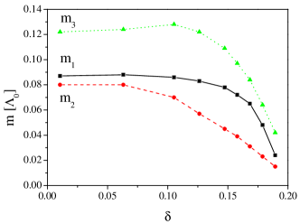
Figure 4: Doping dependence of the gaps in the spin transverse (”1”), total (”2”) and charge transverse (”3”) density modes for the SCd phase. The $m_{\nu}$ are given in units of $\Lambda_{0}$, the initial energy cut-off of the RG procedure (of order $\sim 1eV$).

The plot shows the behavior of the masses versus doping, evaluated with the above formula. One sees that, in the SCd phase, spin gaps go to zero as doping increases and so does the charge antisymmetric mode which has the largest value. The behavior of the gaps for small doping, showing a rather slow decay of their values is in agreement with experimental observations [12]. It is also comparable with predictions obtained after refermionization of the problem and mapping it onto an exactly solvable Gross-Neveu model with SO(8) symmetry [59] (but strict constraints for the Fermi velocities – viz $V_{Fo}=V_{F\pi}$ – and for the ratios of the $g$ couplings at the fixed point have to be fulfilled then). There were also attempts to reduce the low-energy physics of pure $Cu$ two-leg ladder to an SO(5) symmetric case [60, 61]. For our more general system these conditions are usually not met, and spurious phases may even appear if one breaks some of the symmetries, so unfortunately we are not allowed to use these integrable models in our calculations. However some predictions, like the decrease of the gaps with doping and their relative magnitudes are in complete agreement with these special cases.

It is also worthwile pointing out that the values of the two spin gaps are always comparable, so that the approximations that are made when $m_{1}>>m_{2}$ cannot not be used here to calculate the physical properties of our model. This behavior pertains to the range $\delta<\delta_{c1}$; upon approaching $\delta_{c1}=0.2$ from below, gaps tend to close. As we will show next, a different phase, C2S1, emerges for $\delta>\delta_{c2}$. The intermediate range $\delta_{c1}<\delta<\delta_{c2}$ will be discussed separately, when we examine the transition from the $C1S0$ to the $C2S1$ phase.

IV.3 The large doping case

If the asymmetry between the bonding and antibonding bands is larger, $\cot 2\alpha~{}\rightarrow~{}\infty$ and $\cot 2\beta~{}\rightarrow~{}-\infty$, signalling that $B_{o\pi}$ is the eigenbasis for both the spin and charge modes. The RG flow converges very quickly to that fixed point for large dopings, typically when $\delta>0.41$. This corresponds to $\tilde{\alpha}=4.2$, a value that agrees with that found previously in Ref. 19. Interactions are not able to renormalize the ratio of the band Fermi velocities $\gamma$ to one anymore, which confirms that the $B_{o\pi}$ basis is relevant for this regime. In the large doping phase, only $g_{1}\simeq-g_{2}$ are relevant. If one takes into account the rotation of the diagonal basis, which occurs as $\cot 2\alpha$ varies, it appears that this flow produces only one massive spin mode, and we get the $C2S1$ phase predicted by Balents and Fisher [19]; the interaction term which causes this behavior in our case is identical to theirs, once expressed in current density formalism. Using the same method as the one described for low dopings we are able to evaluate the doping dependence of the gap of strongly doped ladders. The result is shown in Fig. 5.

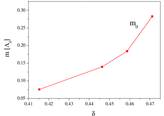
Figure 5: Doping dependence of the gap for the ‘’o” band spin mode. Note that the gap is given in units of the cut-off $\Lambda_{o}$, the value of which decreases quickly when one approaches the bottom of the upper band

One can easily identify the nature of the $C2S1$ phase, in bosonic field language: because the diverging interaction is $g_{o}=g_{1}-g_{2}<0$, the slowest decay of correlations is observed for the CDW operator in the bonding (”o”) band.

For large enough dopings ($\delta>0.41$), a gap will open, even if one starts from very small bare values of the interactions. In the range $0.28<\delta<0.41$, angles still flow to the fixed point limits $\cot 2\alpha(\beta)~{}\rightarrow~{}\infty$, but $g_{1}$ and $g_{2}$ grow very slowly. One needs to choose larger initial values of the bare interactions (but still smaller than the hopping t) and/or assume that one is close to the $C2S1$ region (starting from large $\cot 2\alpha(\beta)$) to find the gap exactly in the relevant spin mode. We conclude that the $C2S1$ phase exists in the entire range $\delta>\delta_{c2}=0.28$ and that, when $0.28<\delta<0.41$, $g_{1}$ and $g_{2}$ are very weakly relevant and thus very sensitive to higher order corrections.

Previously, the existence of a $C2S2$ massless phase was predicted very close to the bottom of the band, (i.e when $\tilde{\alpha}$ becomes quite large). Our calculation, however, shows that the $C2S1$ phase remains stable in that limit. The reason for this difference stems from the choice of initial conditions in Ref. 19. For single orbital ladders, when only on-site Hubbard interactions are included, the initial $g_{2}$ is accidently zero. In our case, the presence of $O$ orbitals always implies a non-zero initial $g_{2}$. This says that the $g_{2}$ term drives the transition, for very large $\tilde{\alpha}$.

At the bottom of the band the dispersion is quadratic, so the bosonization procedure, which requires a linear spectrum around the Fermi points, is not valid. The calculation is done using conventional diagramatic techniques, and it confirms the stability of the $C2S1$ phase with the same relevant coupling as found before.

IV.4 Quantum critical regime between the $C1S0$ and $C2S1$ phases

We now turn to the intermediate regime $\delta_{c1}<\delta<\delta_{c2}$. Our key finding is that in this range, a new, massless, phase exists that had not reported previously, because it is found in the asymmetric limit, i.e when the unit cell contains both $Cu$ and $O$ orbitals.

When one approaches the range $\delta\in(0.2;0.28)$ either from below or from above, gaps appear to go to zero (see Figs. 4 and 5). For $\delta_{c1}<\delta<\delta_{c2}$, one has a line of critical points where the phase is totally massless ($C2S2$). Strong fluctuations, in particular near the critical end points $\delta_{c1}$ and $\delta_{c2}$, cause poor convergence of the RG differential equation system. What is more, the angles Eq. (30) vary significantly in a narrow range of $l$. Using controlled approximations, we obtain an analytical solution that reveals the behavior of the system in this phase: we approach the critical end points from the massive phases; we only keep the dominant couplings, which give us a simplified system of equations. Next we analyze the equations describing the angle rotations, and look for the range were derivatives become large, which takes place close to the fixed points. This gives us a condition for the divergence of $\cot 2\alpha(\beta)$. Once the fixed point is known, one may simplify further the RG differential system. Now computing the RG exponent of each coupling is straightforward and enables us to find those couplings which remain relevant within the range of interest.

Let us first consider $\delta_{c2}=0.28$. This point corresponds to the initial value $\cot 2\alpha=1$. A numerical solution shows that the signs of $(dK_{1}-dK_{2})$ and $B_{12}$ are the same and positive whereas the sign of $(K_{1}-K_{2})$ is negative. From this simple analysis we infer that below this value $|\cot 2\alpha|$ decreases to zero and that above, it increases to infinity. Now, $g_{1}$ and $g_{2}$ are only relevant when $(K_{2}+K_{1}))-P_{1}Q_{1}(K_{2}-K_{1})<2$. $K_{2}$ needs to decrease strongly for this condition to be fulfilled and it is necessary to have nonzero values of $f(P_{1})$ and $Q_{1}$ at the fixed point. This condition corresponds to $|\cot 2\alpha|\rightarrow\infty$, so one sees that below $\delta_{c2}=0.28$ the $g_{1}$ and $g_{2}$ couplings cannot be relevant.

The analysis pertaining to $\delta_{c1}=0.2$ is less straightforward. It involves $|\cot 2\beta|$ and, because $(dK_{3}-dK_{4})$ and $B_{34}$ have opposite signs, it is harder to get the flow correctly. The transition between going to zero and diverging takes place when the absolute value of the two terms are equal. A detailed analysis of the angle dependent part of $d\cot 2\beta$ shows that this happens for $\delta_{c1}=0.2$. When $|\cot 2\beta|\rightarrow\infty$, then $K_{4}^{-1}$, which is much larger then one, influences the renormalization of the $\cos\theta_{c-}$ coupling on equal footing with $K_{3}^{-1}$. This is the reason why these interactions are not relevant anymore.

The above first order RG analysis was done in the vicinity of the critical end points and proves that when $\delta\in(0.2;0.28)$ all interaction terms which are relevant outside are irrelevant inside this range. We have confirmed the above simplified analysis by performing a numerical analysis of the full set of equations which shows that no other coupling is relevant. We see that a $C2S2$ phase is present between the $C1S0$ and $C2S1$ phases. Hints for the possible existence of such state came from numerical studies [62] or from some special models of ladders [63, 64] with specific types of geometries, but we give here a direct proof of the existence of this phase for a generic ladder.

The $C2S2$ phase is a LL where $B_{o\pi}$ is the fixed point eigenbasis for the charge modes and $B_{+\-}$ that for the spin modes. As far as the charge modes are concerned, $K_{4\equiv o}$ is significantly smaller than one, while $K_{3\equiv\pi}$ is very close to one at the fixed point. The spin parameters are both close to one because of the spin rotational symmetry. Thus one expects that correlation functions of band density fluctuations of the form $c_{+/-,o}^{{\dagger}}\sigma_{i}c_{+/-,o}$ have the slowest decay. Logarithmic corrections need to be evaluated, owing to the presence of a (single) marginal coupling $g_{o}=g_{1}-g_{2}>0$. They show that a SDW within the o-band (SDW(o)) is dominant.

IV.5 The influence of $U_{O}$ and $V_{Cu-O}$

Sofar, we have only discussed changes that stem from the presence of $O$ orbitals in the structure. We now turn on the interactions involving the $O$ atoms – $U_{O}$ and/or $V_{Cu-O}$ – and probe whether these additional terms affect or not the phase diagram that we have found previously. In the following, we assume that these interactions do not generate new types of terms in bosonization language, but that they modify the initial parameters of the flow (for a detailed discussion of V-type terms, see for example Ref. 65).

In the $C1S0$ phase, SCd becomes less stable if large $U_{O}$ or $V_{Cu-O}$ are present, but it has always a lower free energy than the OAF phase. When both $U_{O}$ and $V_{Cu-O}$ are present, they seem to have competing effects. One would need to assume a very large attractive bare $V_{Cu-O}$ ($V_{Cu-O}<-3.6U_{Cu}$) in order to stabilize a phase different from SCd. It would be a SCs phase with $\phi_{s-}=0$, $\phi_{s+}=0$, $\theta_{c-}=\pi/2$ and it would be very robust, even if the Fermi level approaches the bottom of the $\pi$ band. The existence of this phase, generated by $V_{Cu-O}$, was first pointed out in Ref. 46. The discussion of Ref. 46 pertains to the half filled case. The nature of the phase transition between the two superconducting phases in ladders was described in detail in Ref. 22, so we are not going to discus this point. In the physical range of values of bare $V_{Cu-O}$, one does not expect SCs to dominate.

In the $C2S1$ phase, $U_{O}$ and $V_{Cu-O}$ do not change the results significantly. Their main influence is that they make the gap smaller. It is to be expected, since the CDW in the ”o” band has an overlap with $O$ atoms sitting between two $Cu$ and introducing electron repulsion on $O$ atoms makes the CDW less stable. For very large attractive $V_{Cu-O}$ the SCs phase re-enters.

In the $C2S2$ phase, increasing $V_{Cu-O}$ has little effect on $\delta_{c2}$ but shifts $\delta_{c1}$ to higher values. For ${{V_{Cu-O}}\over{U_{Cu}}}>1$ the quantum critical line still exists and an unphysically large ratio of $\approx 5$ would be required to suppress the massless phase and to observe a reentrant $C1S0$ phase with superconducting fluctuations. The $\delta_{c1}$ phase boundary is not affected by $U_{O}$ or by $V_{Cu-O}$.

V Discussion and consequences

In this section, we discuss our findings in connection with previous work done on ladders. We also show that the $C2S2$ and $C2S1$ phases possess an orbital current quasi long-range order and we compare our result with other proposals of current patterns for cuprates.

V.1 Differences with the single band case

In the derivation of the RG equations using current algebra, total particle-hole symmetry was assumed. Yet, it was shown [66] that V-type interactions, for instance, can generate terms which break this symmetry at the beginning of the flow. They generate the following terms

• a sine interaction term $g_{2}\sim g_{1o}^{\perp}-g_{1\pi}^{\perp}$

• interactions such as $g_{2o}^{\perp}-g_{2\pi}^{\perp}$ and $g_{1o}^{\parallel}-g_{1\pi}^{\parallel}$, of the form $\nabla\phi_{s+}\nabla\phi_{s-}$, which are included in the definition of the non-diagonal part of the $\hat{K}$ matrix (see Eq. (9)); this implies, for instance, that $P_{1}\neq P_{2}$

• $g_{4}$-type interactions generate different velocities for the spin- and charge modes (per se this is not a relevant perturbation but it enhances the impact of the other two contributions).

When $O$ atoms are included between $Cu$ atoms, even if only $U_{Cu}$ is present, the bare $g_{0}\sim\frac{\lambda_{ao}^{4}}{V_{Fo}}U_{Cu}$ is different from $g_{\pi}\sim\frac{\lambda_{a\pi}^{4}}{V_{F\pi}}U_{Cu}$ and particle-hole symmetry does not hold anymore (in the limit $E\rightarrow\infty$, one has $\lambda_{ao}^{4}-\lambda_{a\pi}^{4}\sim E^{-1}$ and $V_{F}\sim E^{-1}$ so these two effects cancels out and $g_{o}-g_{\pi}$ is still $\sim O(1)$). This shows that it is quite important to include the oxygen atoms in the description of the two-leg ladder.

The system of RG equations that we have derived does not impose such particle-hole symmetry constraint, and hence it may flow to a new fixed point which corresponds to the $C2S2$ phase. At the fixed point, $B_{+-}$ is the diagonal basis for the spin modes and $B_{o\pi}$ is the diagonal basis for the charge modes. It should be emphasized that for all other phases (which had been found previously for single orbital ladders), the diagonal basis at the fixed point is the same for the spin and for the charge modes. The presence of the three bands thus allows the symmetry between spin and charge bases to be relaxed during the flow, and is instrumental in stabilizing the $C2S2$ phase. For the case of a single band, Ref. 67 pointed out that two additional considerations could lead to a significantly modification of the phase diagram obtained in Ref. 19, using a weak coupling perturbative approach. The first one was the inclusion of all interactions, not simply the relevant ones, the second one was the stability of the fixed points. For example in Ref. 67, it was argued that the stability of the $C2S1$ phase was compromised, because of “a spin proximity effect”. However this $C2S1$ phase was found in DMRG numerical studies [68]. In our calculation it is important to note that all possible interactions were taken into account, and we did not impose any a priori symmetry. The presence of the $C2S1$ phase, that we do find in our calculation, is thus intimately connected with the rotation of the spin basis towards the fixed point $B_{o\pi}$ eigenbasis.

At each step, we monitored the spin rotational invariance of the Hamiltonian through Eq. (36) to check that our equations were producing a reliable flow. The result, for the case of small as well as large dopings, is displayed in Fig. 6.

(a)

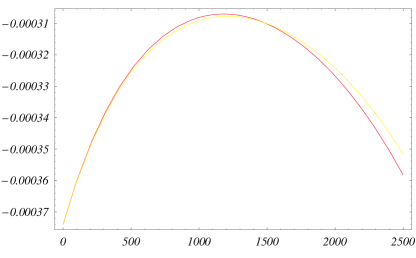
(b)

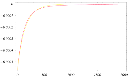
Figure 6: Evolution of $g_{2c}$ (yellow) and $g_{1c}+g_{\parallel c}$ (red) versus number of RG steps, during the flow. It shows that spin rotational symmetry is preserved (a) small $\alpha$ phase (b) large $\alpha$ phase

In addition, in the $C2S1$ phase, there is one single massless spin mode, so that its $K$ parameter must remain equal to one during the flow; we verified that this property does hold.

V.2 Half filling and close to half filling

At half filling, the charge symmetric mode becomes massive. All modes are gapped and spatial correlations decay exponentially. This is due to three relevant umklapp couplings. The spin and charge transverse modes are locked into the same minima as before, and the transition only affects the total charge mode. One may view this transition as a quantum order-disorder Ising type. At half filling the dominant phase is the quantum disordered D-Mott phase, which, upon doping, turns into SCd, its dual counterpart. For large attractive V, an S-Mott phase, the dual counterpart of SCs, dominates at half filling. When we vary the strength of the interactions, the boundaries between these two phases look similar to those found for incommensurate fillings.

The half-filled case for the $Cu$-$O$ ladder was discussed in Ref. 46, both in the weak and in the strong coupling limits. For weak interactions, we may directly compare their results with ours. They used current algebra to treat the low energy physics of ladders with and without outer oxygens (five and seven atoms in the unit cell respectively). In the latter case, a spin-Peierls phase (BDW in Appendix.B) dominates, whereas a D-Mott phase is favored, in the former case. The authors claim that this difference is due to a larger leg to rung anisotropy when outer oxygens are not present. The outer oxygens were taken into account in our model but we nevertheless find a D-Mott phase. More generally, our entire phase diagram is very similar to their “five orbital” case. A possible reason for this discrepancy could be that

their $t_{pp}$ is barely less than the $Cu$-$O$ hopping amplitudes. In our calculations $t_{pp}$ is much smaller, in accordance with LDA studies [49] and with experiments. Recall that, as was described in Section II, whenever $t_{pp}>0.5t$ (or $t_{\bot})$ non bonding p-orbitals become relevant degrees of freedom, and these were not included in our model. Similarly a large initial value of the nearest-neighbor interaction $V$ causes an exchange of the weight of the d and p orbitals in the lowest lying bands during the RG flow. This limit is beyond the range of validity of a simple RG approach.

The strong coupling case (the so called charge-transfer regime) is important, because, for real inorganic materials, $U$ is usually of order 5t. Still, two features of the weak coupling regime remain valid in strong coupling: one is that spin-charge separation holds and two is that in the SCd phase (for instance) there is still an exponential decay of DW operators. A connection between the phase diagrams of these two regimes is often suggested in the literature.

For instance in the case of $Cu$-$O$ ladders close to half filling (the strong coupling case discussion in Ref. 46) a t-J approximation was used. It gave a uniform phase – related to D-Mott – in a broad region of positive $U_{Cu}$-$V_{Cu-O}$ phase space. For large attractive $V_{Cu-O}$, a phase with holes localized around copper atoms is found, probably connected to our SCs ordering. Our phase diagram matches the above description. The SCd phase, which we find close to half filling, is clearly seen in numerical studies. The $C1S0$ phase was connected with this type of ordering in Ref. 27 were it was also shown that the gap preventing a DW-type ordering decreases upon increasing the doping. In Ref. 69 it was found that the region where this phase is stable can be extended up to U=4t. In the t-J model, the rigidity of SCd with respect to a finite difference in the chemical potential of the two-legs was also established [56]. The same type of ordering (rung singlet) also dominates at half filling, for a special choice of parameters giving an SO(5) symmetry [70], since in that case one may solve the model exactly. All these results were obtained for single band ladders; quantitative differences occur when oxygen atoms are included in the unit cell, and these were analysed in a numerical study [47].

Few studies were devoted to the intermediate and large doping regimes; we discussed the $C2S1$ phase (see above), and, as far as the $C2S2$ phase is concerned, a DMRG study [62] suggested the existence of such gapless phase well inside the bands for a zig-zag ladder; the occurrence of a massless phase in the strong interaction limit would be certainly remarkable.

V.3 Orbital current patterns at intermediate and large dopings

In the previous sections, we had set $t_{pp}=0$. We now assess the influence of this hopping term on the phase diagram. As long as $t_{pp}<\emph{0.5t}$, our RG method remains valid, and only the initial parameters are changing with $t_{pp}$. As we increase $t_{pp}$, we note that $\tilde{\alpha}$ increases for a given doping, but that both $\delta_{c1}$ and $\delta_{c2}$ are decreasing. For $t_{pp}=0.5$, their values are about half that quoted for $t_{pp}=0$. A negative $t_{pp}$ (the electron-doped case) has the opposite effect. This influence of $t_{pp}>0$ can be understood as an increased asymmetry between bands.

The phase diagram, which summarizes our study of the $Cu$-$O$ ladder for carrier concentrations between half filling down to the bottom of the “upper” band, is shown in Fig. 7.

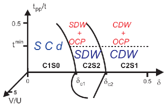
Figure 7: Phase diagram of two-leg Hubbard ladders versus doping for $U_{Cu}>0$. $\delta=0$ corresponds to the half filled case; umklapp terms which open up a gap in the charge symmetric mode are not included here; DW+OCP denotes phases with orbital current pattern (OCP) on top of a spin- (SDW) or a charge- (CDW) density wave.

A spectacular effect of $t_{pp}$ is that it leads to new types of current loops, involving oxygen sites; the range of parameters where orbital current patterns (OCP) dominate is seen in Fig. 7.

A finite $t_{pp}$ allows direct current flows between oxygen atoms, giving rise to additional patterns, enclosed inside the elementary cell. One of these preserves the mirror symmetry on the $\sigma$ axis (the axis parallel to the chain direction and passing through the mid-rung oxygens), and it is of special importance. This is because we have shown that, at least for moderate dopings, operators in the $o$ band dominate. The current operator between two atoms ”a” and ”b” is defined as $j_{a-b}=\sum_{\alpha,\alpha^{\prime}}\psi_{\alpha a}^{{\dagger}}\psi_{\alpha^{\prime}b}-\psi_{\alpha^{\prime}b}^{{\dagger}}\psi_{\alpha a}$ (we sum over band indices) and the total current pattern operator is given as a sum of currents on each bond. For symmetry reasons, if the current pattern has a mirror symmetry along $\sigma$, then the total current operator has the form of a particle-hole fluctuation in the $o$ band.

Two conditions must be met in order to get a dominant contribution: the pattern must form closed loops originating from and ending at $Cu$ atoms and it has to possess a mirror symmetry with respect to the plane containing $\sigma$ and perpendicular to the plane of the ladder. One of the current patterns preserves both of the required constrains and, since it is similar to a configuration proposed by Varma, we call it ”VarmaI”-type (Fig. 8). Then, because the current operator has the same dependence on phase fields as the DW operator, these fluctuations have the same power law decay. Computing their amplitude will tell us which type of order dominates.

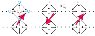
Figure 8: Current pattern in the $C2S2$ phase. It has a mirror symmetry with respect to the $\sigma$ axis plus an additional SDW. The modulation has an incommensurate spatial periodicity ${2k}^{-1}_{F0}$

In the large doping regime ($C2S1$), we compare the amplitude of the ”normal” CDW and of the OCP+CDW. The amplitude of the latter is found by summing current operator contributions for loops with one $Cu$ and two $O$ atoms. We use the mirror symmetry and add first equivalent pairs of currents. Each of these pairs gives a contribution proportional to $t_{ij}Im(\lambda_{a\alpha}\lambda_{bi\alpha})$ or $t_{ij}Im(\lambda_{bj\alpha}\lambda_{bi\alpha})$, where $t_{ij}$ is the hopping parameter between the relevant atoms. We emphasize once again that, in the single ($Cu$) orbital case, $\lambda_{a\alpha}=1$ so that the current operator between $Cu$ atoms has the usual interband form. It is the presence of oxygens that gives $Im(\lambda_{a\alpha}\lambda_{bi\alpha}\neq 0$, allowing the geometry of a Varma-type pattern to appear in the theory.

A numerical calculation shows that these quantities are of order one and change only by a few percent when the doping increases from 0.25 to the value of $\delta$ at the bottom of the band. The result of this procedure (the amplitudes of the currents determined by the products of $\lambda_{ij}$ coefficients) is shown in Fig. 9; since it is easier to visualize a commensurate pattern, we chose $\delta=0.9$ such that $k_{Fo}=1/4$ (note that only the “0” band would cross the Fermi level for such a large value of the doping).

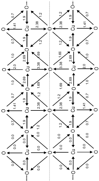
Figure 9: Current amplitudes within the o-band, given in $t_{pp}$ units. For this particular doping, the pattern has an 8-cell periodicity; The figure shows half a period (the other half is simply obtained by repeating the amplitude pattern and reversing all the signs)

Due to current conservation, the weakest link between atoms determines the maximum value of the current. It is clear that the magnitude of $t_{pp}$ determines whether or not the OCP+CDW state may exist. Since the total amplitude is proportional to $2t_{pp}\sum_{ij}Im(\lambda_{bj\alpha}\lambda_{bi\alpha})$ multiplied by the number of links, it is straightforward to obtain a threshold value $t_{pp}^{(min)}\approx 0.3t$ above which the OCP+CDW phase dominates.

Varma’s work was concerned with the strong coupling regime in 2D, and the stability of the current patterns was studied in mean-field theory. The fact that we were able to find such a state in 1D, in the weak coupling limit and with purely repulsive interactions, gives an interesting perspective on the possible existence of such orbital currents. Note that a type ordering similar to the one we find (current+DW) has been suggested in numerical studies of two-leg ladders [28, 42]. We will return to this issue in the last part of this section, where we make a contact with strong coupling results. The statement about the existence of OCP states given above, obviously holds also for the $C2S2$ phase, where CDW fluctuations are replaced by SDW fluctuations (Fig. 8). We also note two differences between our orbital current states and Varma’s: in our case, the structure is incommensurate (the modulation is doping dependent) and we get an additional DW modulation. Hence, the OCP+DW state also share similarities with the DDW phase [43]. The main point is that introducing $t_{pp}$ gives the possibility of new types of current loops involving oxygen sites. Phases with time reversal symmetry breaking have been widely investigated, but, for single orbital models, currents flow along $Cu$ square plaquettes, giving rise to the OAF state. As was shown in detail by Fjaerestad and Marston [71] they are described by inter-band creation-annihilation process $\sim\psi_{o}^{{\dagger}}\psi_{\pi}$. The order operator in bosonization language is given in Appendix D (it is the $\hat{O_{OAF}}(r)$ operator) and, this type of quasi-long range order is stable provided one introduces an attractive $V_{Cu-Cu}$.

What about current patterns in the strong coupling regime? This issue was investigated numerically. One paper [28] showed that if time reversal symmetry is artificially broken by adding a magnetic field, one promotes a state with OAF currents and a CDW modulation for the two-leg ladder, very similar to the one suggested in Sec. IV. Another [42] considered variants of t-J models, in hopes of finding current pattern phases. Although somewhat artificial values were assigned to some of the parameters, this study suggested that quasi long-range order of the current patterns could be obtained provided one changed the internal description of the rung. Furthermore, the current pattern is accompanied by a charge density wave structure.

It should be pointed out that both papers established a direct connection between the strong and the weak coupling regimes. For example, Ref. 42 showed that the spatial decay of current-current correlations is similar in regions of parameter space corresponding to weak or large coupling RG. This paper also emphasizes that, in order to obtain current patterns, one needs to go beyond theories using properties of SO(5) symmetric models. This confirms our findings, that new physics emerges in formalisms where symmetry breaking is a priori allowed.

V.4 Experimental systems

Experimentally, it is rather difficult to vary the doping in ladder compounds, and the large doping regime is still inaccessible [72]. Furthermore, different methods (NMR, optical conductivity and X-ray measurements) yield different values of the doping for a given system [73]. One of the most interesting compounds, $Sr_{14-x}Ca_{x}Cu_{24}O_{41}$, contains both chains and ladders, and it was shown that a change in pressure may cause a charge transfer between the two [8]. Calcium is also a factor that affects the carrier content of the ladder. In the low doping regime, this system displays spin-gaps, as is well established in many NMR studies; this will be discussed in detail in the next section. As far as charge degree of freedoms are concerned, the situation is more complicated. There are optical conductivity measurements showing CDW ordering in these systems at ambient pressure [74]. This kind of ordering may be due to a large $V_{Cu-Cu}$ [75] not taken into account in our model or to inter-ladder electrostatic interactions. The SCd phase appears under pressure, with a maximum temperature of order 10K for an optimal pressure of 3.5 GPa. The role of pressure in this transition is not clear: it may change the bandwidth, the couplings between ladders, the screening of the intra- or inter- ladder interactions, or the doping. Recently[76, 77], soft X-ray measurements were performed for this system. Their main conclusion is that an insulating “ hole crystal” phase exists for commensurate fillings. It is suggested that this phase melts for other dopings. The authors interpret their findings by invoking strong on-rung hole pairing. This analysis supports the picture that emerges from our study of the low doping regime.

VI NMR properties

VI.1 Spin susceptibility and NMR relaxation rate

The spin operator with momentum $q$ is defined as

$$S_{m}^{i}(\textbf{q})\equiv\frac{1}{2}\sum_{\textbf{k}\sigma 1\sigma 2}c^{{\dagger}}_{m\sigma 1}(\textbf{k}+\textbf{q})\widehat{\sigma^{i}}c_{m\sigma 2}(\textbf{k})$$ (40)

where $c\equiv a,b$ (respectively the annihilation operator of a hole on $Cu$ or on $O$) and $\widehat{\sigma^{i}}$ is a Pauli matrix. From linear response theory, the time-ordered susceptibility reads

$$\chi_{m^{\prime}m}^{i}(\textbf{q},\imath\omega_{n})\equiv\frac{1}{2L}\int_{0}^{\beta}d\tau\langle T_{\tau}S_{m^{\prime}}^{i}(\textbf{q},\tau)S_{m}^{i}(\textbf{-q},0)\rangle\exp(\imath\omega_{n}\tau)$$ (41)

The above function is defined only for Matsubara frequencies $\omega_{n}$; taking the analytical continuation, one obtains the retarded susceptibility $\chi_{m^{\prime}m}^{R}$ [78] and hence derive [50] analytical expressions for the measured NMR properties of the system.

The NMR signal comes from a contact interaction between a nucleus and the surrounding cloud of electrons in an s-orbital state.

The temperature dependence of the shift in (Zeeman) frequency of the m-th nucleus stems from hoppings of carriers from the m-th atom s-orbital to the highest occupied molecular orbital p or d orbital of the neighbouring sites. Thus, the Knight shift is

$$\bar{K}^{i}_{m}=\frac{C_{m}}{\gamma_{m}\gamma_{e}\hbar^{2}}\sum_{m^{\prime}}\chi_{m^{\prime}m}^{Ri}(\textbf{p}\rightarrow 0,\omega=0)$$ (42)

where the summation is taken over all neighboring d-Cu and p-O orbitals. The overlap coefficients $\widetilde{\lambda_{m\alpha}}$, which enter $\chi_{m,m^{\prime}}$, are evaluated using first order perturbation theory; we include hoppings between a s-Cu orbital and a p-O orbital on the neighbor sites or a d-Cu orbital on next-nearest neighbor sites, as well as hoppings between a s-O orbital and a d-Cu orbital on neighboring sites.

The spin-lattice relaxation rate is also affected by the electronic environment. The signal measured on the m-th nucleus is given by

$$(\frac{1}{T_{1m}})^{i}=\frac{C^{2}_{m}}{\gamma_{m}\gamma_{e}\hbar^{2}\beta}\sum_{\textbf{p}}\frac{Im[\chi^{Ri}_{mm}(\textbf{q},\omega_{Zm})]}{\omega_{Zm}}$$ (43)

In the following, we omit the ‘’i” subscripts, because we are working with spin-rotationally invariant models. Taking into account the fact that the Fermi surface consists of pairs of points of the form $\pm k_{F}$, the sum in $\frac{1}{T_{1}}$ can be divided into two independent parts: a uniform piece (q around $k_{\|}=0$) and a staggered piece (q around $k_{\|}=2k_{F}$).

Using the $\widetilde{\lambda_{m\alpha}}$ allows us to connect the time-ordered correlation functions $R_{\alpha}(r(x,\tau))$ of carriers in band $\alpha$ (they are introduced in the bosonic phase field language), with the $R_{m^{\prime}m}(r(x,\tau))$ defined for a site basis

$$R_{m^{\prime}m}(r(x,\tau))=|\widetilde{\lambda_{m^{\prime}o}}|^{2}|\widetilde{\lambda_{mo}}|^{2}R_{o}(r(x,\tau))+\\ |\widetilde{\lambda_{m^{\prime}\pi}}|^{2}|\widetilde{\lambda_{m\pi}}|^{2}R_{\pi}(r(x,\tau))$$ (44)

In order to get the retarded $\chi^{R}_{m,m^{\prime}}(q,\omega)$ entering Eqs. (42,43), we use the fact that correlations for spin operators and for their complex conjugates are equal, and we simply obtain the retarded spin susceptibility by a Wick rotation [79]:

$$\chi_{m^{\prime}m}^{Ri}(x,t)=2\theta(t)Im[R_{m^{\prime}m}(r(x,\tau))]_{\tau=\imath t+\delta}$$ (45)

followed by Fourier transforming the last function.

Because of conformal symmetry in our 1D quantum theory, results for zero temperature correlations can be extended to finite temperatures by simply substituting for the complex coordinates the following expression

$$r_{\nu}(x,\tau,\beta)=\frac{u_{\nu}\beta}{\pi}\sqrt{\sinh(\frac{x-\imath u_{\nu}\tau}{\frac{u_{\nu}\beta}{\pi}})\sinh(\frac{x+\imath u_{\nu}\tau}{\frac{u_{\nu}\beta}{\pi}})}$$ (46)

This substitution $r_{\nu}(x,\tau)\rightarrow r_{\nu}(x,\tau,\beta)$ gives us the temperature dependence of the susceptibilities.

This procedure is valid both for the uniform and for the staggered parts of the magnetization. We write the time ordered correlation functions $R_{\alpha}(r(x,\tau))$ in each band in terms of diagonal modes $R_{\nu}(r(x,\tau))=F[\phi_{\nu}]$ for the staggered and the uniform part, separately. The form of $F[\phi_{\nu}]$ depends on whether the $\nu-th$ LL mode is massless or massive and it will be presented below. Given $F[\phi_{\nu}]$, the substitution 46 allows us to obtain the temperature dependence of $K_{m}$ and $T_{1m}^{-1}$, but as the temperature increases, the form of $F[\phi_{\nu}]$ is changing. Generally it is assumed that above the temperature $T_{\nu}$ corresponding to the value of the gap $\Delta_{\nu}$, thermal fluctuations make the $\nu$-th mode massless.For example, at $T=0$, in the $C1S0$ phase, one starts with three gapped modes (two for the spin and, one for the charge); we increase $T$ until the energy of the first gap $\Delta_{s+}$ is reached. Above the corresponding temperature $T_{s+}$ we may consider that there is effectively one gapped and one gapless spin mode, and similarly for the charge sector. The others gaps ($\Delta_{s-}$ and $\Delta_{c-}$) will successively close at temperatures $T_{s-}$ and $T_{c-}$.

VI.2 Doping dependence of the NMR signals

A number of papers [80, 81, 82],were devoted to the computation of magnetic properties of two-leg ladders assuming symmetry entanglement at the fixed point (SO(5) or SO(8)). Yet, following the discussion in section IV, we use simpler, approximate, methods which nevertheless have a wider range of validity.

VI.2.1 Uniform part

For the uniform magnetization, only spin correlations need to be taken into account. Because the spin density is generally related to the spin phase field $\sigma(x)=\frac{1}{\pi}\nabla~{}\phi_{\sigma}(x)$, the zero momentum part of $\bar{R}_{o}$ is a linear combination of bosonic correlations calculated in the diagonal basis $\bar{R}_{\nu}(r)$. In the massless case it is known from LL properties and given by

$$\bar{R}_{\nu}=\frac{1}{r_{i}^{2}}$$ (47)

The contribution to NMR of these power laws has been evaluated many times before in the literature. One gets a $T^{0}$ dependence for the Knight shift and $T^{1}$ for the relaxation rate. One may improve these result both in the high- and low energy limits. At low energies, logarithmic corrections from relevant and marginal couplings $g(\Lambda)$ (where the energy scale $\Lambda$ may be related to the temperature) should be taken into account. Then, $g_{1c}$ and $g_{2c}$ contribute to the o and $\pi$ bands, $g_{1}+g_{2}$ to the o band and $g_{1}+g_{2}$ to the $\pi$ band. At high energies, the curvature of the bands may be taken into account using an RPA approximation, following Refs. [21, 83].

In the massive case we use the massive Gaussian model to obtain fluctuations around the static quasi-classical solution (equilibrium position) and this leads to

$$\bar{R}_{\nu}=K_{i}(\kappa_{0}(m_{i}r_{i})+\kappa_{2}(m_{i}r_{i}))$$ (48)

where we have used the fact that for harmonic fluctuations around the soliton $\delta\phi_{i}(x)\equiv\phi_{i}(x)-\phi_{oi}(x)$, correlations are given by a Bessel function $\langle\delta\phi_{i}(r)\delta\phi_{i}(0)\rangle\simeq\kappa_{0}(m_{i}r)$. A first order expansion, valid for large r, gives exactly the same expression as that found in exact calculations [84, 85]. One needs to evaluate the following integrals (the exact formulas for the LL $\chi(k,\omega)$ are known [86] but it is not necessary to use them here)

$$\frac{1}{T_{1m}}=\int dt\sum_{x_{0}}\digamma[\widetilde{\lambda_{m\nu}}^{2}(x_{0})]R(x_{0},t)$$ (49)

$$\bar{K}_{m}=\widetilde{\lambda_{m\nu}}^{2}(k=0)(\sum_{m^{\prime}}\widetilde{\lambda_{m\nu}}^{2}(k=0))\int dtdxR(x,t)$$ (50)

where the summation over $x_{0}$ accounts for the momentum dependence of $\widetilde{\lambda_{m\nu}}(k)$. For the uniform part, integrals can be calculated analytically

$$\frac{K_{i}m_{i}V_{i}}{\pi}(\kappa_{0}(m_{i}r_{i})\frac{\cosh(\frac{\pi(x-\imath V_{i}t)}{V_{i}\beta})\sinh(\frac{\pi(x+\imath V_{i}t)}{V_{i}\beta})-\sinh(\frac{\pi(x-\imath V_{i}t)}{V_{i}\beta})\cosh(\frac{\pi(x+\imath V_{i}t)}{V_{i}\beta})}{\sqrt{\sinh(\frac{\pi(x-\imath V_{i}t)}{V_{i}\beta})\sinh(\frac{\pi(x+\imath V_{i}t)}{V_{i}\beta})}}\mid_{b}^{c}$$ (51)

the appropriate bound b,c is chosen for the Knight shift or for the relaxation rate, and depends on whether one integrates over a time or a space-time domain.

The results for Knight shifts, calculated for different atoms and different dopings, are shown in Figs. 10 and 11. The discussion of the relaxation rates is postponed until after the evaluation of the staggered part, because the quantity which is measured in experiments is the sum of the uniform and the staggered parts of the relaxation rate.

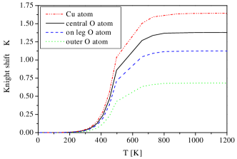
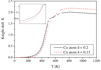
Figure 10: Temperature dependence of the Knight shifts for (a) the different atoms in the elementary cell and (b) different dopings in the $C1S0$ phase. The activation gap at low $T$ is shown in the inset

For the $C1S0$ phase, an activated behavior $exp(-\frac{\Delta}{T})$ is seen for the Knight shifts of all the atoms. This shows clearly on the logarithmic plots shown in the inset of Fig. 10. However let us stress that in the $C1S0$ case we have two spin gaps, so one expects a more complicated shape than a simple straight line. For higher temperatures the Knight shift saturates to a constant value. As is expected for the uniform susceptibility, the responses of the different atoms are similar, only their amplitudes are different (this is because of the $|\widetilde{\lambda_{m\nu}}|^{2}$ coefficients). For larger dopings there are less electrons in the conduction band, and their velocity is smaller, so the saturation value also decreases. As the doping increases, spin gaps decrease and curves saturate at a lower $T$ until we reach the quantum critical point (QCP) at $\delta=\delta_{c1}$. This behavior for the susceptibility was described in Ref. 21. In their case, a QCP appears in the presence of $V_{Cu-Cu}$; in our case, doping drives the transition.

(a)

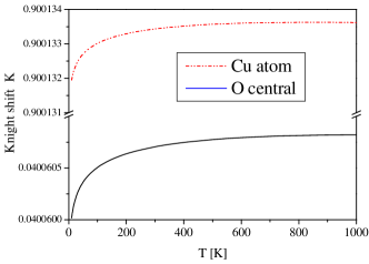
(b)

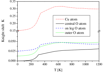
Figure 11: Temperature dependence of the Knight shifts for the different atoms in the elementary cell (a) in the $C2S2$ phase and (b) in the $C2S1$ phase

For the $C2S1$ phase, we obtain a finite susceptibility even at zero temperature. This feature comes from the massless spin mode. The central oxygen atom which is only coupled to the gapped band does not give a finite susceptibility at T=0. For the second, massive, mode we observe a behavior similar to the one described above for the $C1S0$ phase, with the single activation gap shown on the inset of Fig. 10b for two dopings.

For the intermediate doping $C2S2$ phase, including logarithmic corrections is the only way to generate some weak $T$ dependence. They arise mainly from the presence of the marginal $g_{1}$ and $g_{2}$ terms. Their influence on the uniform susceptibility was described in detail in Refs. [21, 87]. Differences in the amplitudes of the Knight shifts for the various atoms in the elementary cell stay pretty much the same from one phase to the next, since these amplitudes are simply determined by $\widetilde{\lambda}$ coefficients.

VI.2.2 Staggered part

For $q=2k_{F}$, both the spin and charge parts contribute to the band correlation functions. The band $\tilde{R}_{o/\pi}$ with $2k_{F}$ wave vector is a product of a spin and and a charge part, $R_{\alpha}=R_{\alpha}^{\sigma}\cdot R_{\alpha}^{\rho}$. The form of $F[\phi_{\nu}]$ depends on the fixed point eigenbasis for the angles and on the possible existence of gaps.

The expression for the gapped spin phase was obtained using the expression for the $2k_{F}$ part of the spin density operator correlations which is given by $\langle O_{o/\pi SDW}(r)O_{o/\pi SDW}(0)\rangle^{2k_{F}}\sim\cos(\phi_{1}\pm\phi_{2})$. The last form could be evaluated using the fact that $\phi_{i}=\phi_{oi}+\delta\phi_{i}$ where the fluctuations of $\delta\phi_{i}$ are described by a massive Gaussian model, as was shown in the case of the uniform part. For gapped spin $(\sigma)$ modes there are two possibilities

$$\tilde{R}_{o/\pi}^{\sigma}=\sinh(K_{2}\kappa_{0}(m_{2}r_{2})\pm K_{1}\kappa_{0}(m_{1}r_{1}))(m_{2}a)^{K_{2}}(m_{1}a)^{K_{1}}\\ \textrm{for the \emph{C1S0} phase}\\ \tilde{R}_{o}^{\sigma}=\sinh(K_{2}\kappa_{0}(m_{2}r_{2}))(m_{2}a)^{K_{2}}\\ \textrm{for the \emph{C2S1} phase}$$ (52)

In the gapless case, one gets a power law behavior; for the high-$T$ limit of the $C1S0$ phase, where the $B_{+-}$ eigenbasis is relevant, we find

$$\tilde{R}_{\alpha}=(\frac{1}{r_{i}})^{K_{i}/2}(\frac{1}{r_{j}})^{K_{j}/2}$$ (53)

where $\alpha$ corresponds to the band index and $i=1,3$, $j=2,4$ are the LL modes;

For the $C1S0$ phase, the charge mode is only partially gapped: the field $\theta_{3}$ is locked so the charge antisymmetric mode does not give any contribution to SDW, but the massless ,“4” (charge symmetric) mode gives a power law contribution

$$\tilde{R}_{o/\pi}^{\rho}=(\frac{1}{r})^{K_{4}/2}$$ (54)

For the other phases, both charge modes are massless and in this case, $B_{o\pi}$ is the fixed point basis, and we have

$$\tilde{R}_{o}=(\frac{1}{r_{j}})^{K_{4}}$$ (55)

$$\tilde{R}_{\pi}=(\frac{1}{r_{i}})^{K_{3}}$$ (56)

For the spin part in the $C2S1$ phase, one substitutes $K_{1},K_{2}$ to $K_{3},K_{4}$. The amplitudes of $\tilde{R}_{\alpha}$ on different atoms need to be calculated. Once again $\widetilde{\lambda_{m\alpha}}(k)$ are involved, however for those atoms with neighbors along the ladder (on-leg $Cu$ and $O$ atoms) these coefficients are different, because of phase factors at $k=2k_{F}$ which cause cancellations in some contributions of neighboring atoms. Another possible factor may cause differences between atoms in the elementary cell. Following Ref. 88, one may assume that, below a characteristic distance $x<L_{\delta}=\delta^{-1}$, umklapp terms are relevant and that they open up a gap in the charge symmetric channel. This massive charge correlation affects the staggered part of the magnetic susceptibility, and yields an expression similar to Eq. (52) (with $\cosh$ instead of $\sinh$). For on-leg oxygens, which sit between two $Cu$ along the ladder, one recovers a $\sinh$ instead of a $\cosh$. This produces different amplitudes $\tilde{R}_{o/\pi}^{\rho}(L)$ for $Cu$ and for $O$ on-leg atoms, provided $L_{\delta}>m_{4}^{-1}$. We have made the calculation for the half filled case, and the result is that $m_{4}$ is of the same order as $m_{2}$, so for dopings larger than $0.05$ this effect should not play any role.

Once band correlation functions are known one may follow exactly the same procedure as in the uniform case in order to obtain the temperature dependence of $\frac{1}{T_{1}}$.

VI.2.3 Total relaxation rate

The plots in Fig . 12 shows $1/T_{1}$ for different atoms in the elementary cell. They were obtained by numerical integration of Eq. (52) and adding the result to that computed for the uniform part.

As for the Knight shifts, the difference between atoms are caused mainly by the different $\widetilde{\lambda_{m\alpha}}$ coefficients. However these coefficients can be different for the staggered part and for the uniform part.

The first observation is the linear dependence of $\frac{1}{T_{1}}$ at high temperatures for all atoms, for all dopings. The Knight shift saturates in this temperature range to a constant value and this is in accordance with the Korringa law. For the $C2S2$ phase we observe the linear dependence as expected for a massless LL with all K parameters close to one.

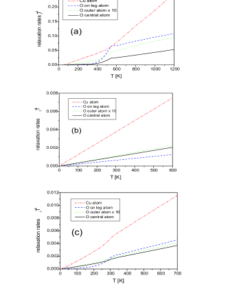
Figure 12: Temperature dependence of the relaxation rates for the different atoms in the elementary cell (a) in the $C1S0$ phase,(b) in the $C2S2$ phase, (c) in the $C2S1$ phase

The second main conclusion is that processes involving large $k_{\parallel}$ transfers can strongly affect the measured rates, especially for temperatures comparable with the spin gaps, as previously reported [89]. One observes only small differences between atoms in the elementary cell at low $T$. The difference in the relaxation rate of a $Cu$ nucleus compared with a central $O$ nucleus comes form the fact that the latter may only relax through processes in the “$\pi$” band, while, for the former, both bands contribute. The difference between on-leg atoms and atoms sitting at other locations comes from the fact that the staggered part contribution of the former nucleus is very small, as it is suppressed by the opposite contributions of the two neighboring $Cu$ atoms. The low-$T$ activation behavior (in the $C2S1$ and $C1S0$ phases) is then clearly seen on these on-leg $O$ sites.

Two points should be kept in mind when comparing our results with experiments. First our $\Lambda_{0}$ is of order 0.5 eV, so that the largest charge antisymmetric gap is of order 700K; observing it would be experimentally challenging, and it would be even harder to reach the Korringa regime predicted at higher $T$. Second, our calculations were made in the phase where SCd fluctuations dominate. Thus experiments done at large pressures would be the most relevant to compare our findings with.

Aside from the above caveats, the results of our calculations seem to be in very reasonable agreement with experiments [10, 9].

VII Conclusions

Our study has clearly shown that including oxygen atoms in the structure produces significant changes in the ground state phase diagram of doped, $Cu$-$O$, two-leg Hubbard ladders. This result is fully consistent with DMRG studies suggesting that there are quantitative differences between models which include $O$ atoms and models which do not, even close to half-filling. The massless $C2S2$ phase is of special importance in that respect. A Varma-like phase with incommensurate orbital current patterns and additional density wave characterize the ground state structure at intermediate and large dopings. Signatures of these states can be seen in NMR experiments probing the various nuclei in the cell.

We see important differences between $Cu$ and $Cu$-$O$ ladders in the weak interaction limit ($U<\epsilon$), but numerical approaches which can investigate the opposite limit as well suggest that these differences do survive for $U>\epsilon$. This invites further analytical studies of the two-leg $Cu$-$O$ Hubbard ladders in the large $U$ limit.

Appendix A Coupling constants

Initial conditions for the non-linear terms are

$$\begin{split}g_{1c}^{o}&=4f(1,2,1,2,1)\\ g_{1a}^{o}&=4f(1,2,2,1,1)\\ g_{2c}^{o}&=4f(1,2,1,2,-1)\\ g_{\parallel c}^{o}&=4(f(1,2,1,2,1)-f(1,2,1,2,-1))\\ g_{1}^{o}&=\frac{2f(1,1,1,1,1)}{V_{Fo}}+\frac{2f(2,2,2,2,1)}{V_{F\pi}}\\ g_{2}^{o}&=\frac{2f(1,1,1,1,1)}{V_{Fo}}-\frac{2f(2,2,2,2,1)}{V_{F\pi}}\\ g_{4a}^{o}&=4f(1,2,2,1,-1)\end{split}$$ (57)

where the function $f(k,l,m,n,p)$ converts the interactions given in the atomic basis ($U_{Cu},U_{O},V_{Cu-O}$) into band “g-ology” interactions.

$$f(k,l,m,n,p)=\sum_{i,j}\lambda_{ik}^{\ast}\lambda_{il}^{\ast}\lambda_{jm}\lambda_{jn}(V^{intra}+\\ V^{inter}\cos(k_{Fm}-p\cdot k_{Fn}))$$ (58)

The summation is taken over all the atoms in the elementary cell. $V^{intra}$ denotes interactions within the elementary cell, and $V^{inter}$ is $V_{Cu-O}$, since one of the atoms is outside the elementary cell, as in Ref. 46. Initial values for $K$ and $\cot(\alpha),\cot(\beta)$ are evaluated as follows: starting from Eq. (12), one performs a $S(\pi/4)$ rotation. In this $B_{+-}$ basis, $\hat{K}$ can be calculated by simply solving a matrix equation. The initial $K_{\nu}$ are given by the eigenvalues of this matrix, and $\cot(\alpha),\cot(\beta)$ are the ratios of non-diagonal terms to the difference of diagonal ones. For example: $\cot(\alpha)=2B_{s+,s-}/(K_{s-}-K_{s+})$.

The system of RG differential equations is solved by means of an iterative method.

If $\cot(\alpha)$ (or$\cot(\beta)$) becomes very large during the flow, we stop the flow at some point, introduce the tangent of the angles instead of the cotangent, and then resume the iteration scheme. In this way, we are able to isolate divergences of the prefactors in some of the cosine terms, which cause gaps to open and affect observables.

Appendix B Derivation of the RG equations

B.1 Flow of the diagonal basis

To second order in perturbation, one finds the corrections $dK_{1}$, $dK_{2}$, $dK_{3}$, $dK_{4}$ to the LL parameters, and the non-diagonal terms $dB_{12}$, $dB_{34}$. These non-diagonal terms signal that, after the RG step, $B_{o}$ is no longer a diagonal basis. We then go back to the $B_{+-}$ basis, using the transformation $S^{-1}$. In this basis, off-diagonal terms have been incremented by small amounts during the RG step. For instance

$$dB_{s-s+}=-\frac{1}{2}(dK_{1}-dK_{2})\cos 2\alpha+dB_{12}\sin 2\alpha$$ (59)

Diagonal terms also undergo infinitesimal variations

$$dK_{s-(s+)}=\frac{1}{2}(dK_{1}+dK_{2})\pm\frac{1}{2}(2dB_{12}\cos 2\alpha+(dK_{1}-dK_{2})\sin 2\alpha)$$ (60)

Similar expressions hold for the charge modes when we perform the substitutions $s\to c$, $1\to 3$, $2\to 4$, $\alpha\to\beta$ in the equations above.

The new matrix is diagonalized by the operator $S(\alpha+d\alpha,\beta+d\beta)$, where the angle $d\alpha$, which account for the $dB_{\mu-\mu+}$ and $dK_{\mu-(\mu+)}$ variations ($\mu=c,s$), indicate a rotation of $B_{o}$. This idea is summarized in the diagram shown in Fig. 3.

We now determine the renormalization flow of the angles $\alpha$ and $\beta$. In the spin sector, the diagonalization condition is written in terms of $K_{s-(s+)}$ and $B_{s-s+}$

$$\frac{1}{2}(K_{s-}-K_{s+})\cos 2\alpha+B_{s-s+}\sin 2\alpha=0$$ (61)

One differentiates the above equation in order to relate $d\alpha$, $K_{s-(s+)}$ and $B_{s-s+}$:

$$-\frac{d2\alpha}{\sin^{2}2\alpha}=\frac{2}{K_{s-}-K_{s+}}\cdot\\ \frac{\frac{1}{2}(dK_{s-}-dK_{s+})\cos 2\alpha-dB_{s-s+}\sin 2\alpha}{(\sin^{2}2\alpha-\cos^{2}2\alpha)\sin 2\alpha}$$ (62)

In the diagonal basis this equation reads

$$d\cot 2\alpha=-\frac{1}{K_{1}-K_{2}}((dK_{1}-dK_{2})\frac{2\sin 2\alpha\cos 2\alpha}{\sin^{2}2\alpha-\cos^{2}2\alpha}-\\ dB_{12}\frac{-\sin^{2}2\alpha+\cos^{2}2\alpha}{\sin^{2}2\alpha-\cos^{2}2\alpha})$$ (63)

where the differentials of the LL parameters are known in the diagonal basis. They were obtained to second order in perturbation, and the $dK_{\nu}$, which we use here, were given in Sec. III.1. In the charge sector, we obtain the equivalent set of equations with the changes $s\to c$, $1\to 3$, $2\to 4$, $\alpha\to\beta$. The additional expressions for the differentials of off-diagonal terms are obtained in a similar way, giving, for the case of a generic filling

$$\begin{split}dB_{12}&=P_{1}Q_{1}((g_{1a}^{2}+g_{\parallel c}^{2}+G_{t}^{2})-\\ &K_{1}K_{2}(g_{1a}^{2}+g_{1c}^{2}+g_{2c}^{2}+G_{p}^{2}))-K_{1}K_{2}h(P_{1})g_{1}g_{2}\\ dB_{34}&=P_{2}Q_{2}(g_{1c}^{2}+g_{2c}^{2}+g_{\parallel c}^{2})\end{split}$$ (64)

where $h(P_{1})=((P_{1}Q_{1})^{2}+0.25(P_{1}^{2}-Q_{1}^{2}))^{-1}$.

B.2 First order correction to $g_{1}$, $g_{2}$

Setting $g_{1}=g_{1d}+g_{1d^{\prime}}$ and $g_{2}=g_{1d}-g_{1d^{\prime}}$, the Hamiltonian reads

$$H=H_{LL}+g_{1}\int dr\cos(2\phi_{s-})\cos(2\phi_{s+})+\\ g_{2}\int dr\sin(2\phi_{s-})\sin(2\phi_{s+})$$ (65)

In order to simplify the RG calculation, we first solve this problem in the total/transverse basis where the averages over the high energy terms are $\langle\phi_{s-}(r)^{2}\rangle_{h}=K_{s-}dl$, $\langle\phi_{s+}(r)^{2}\rangle_{h}=K_{s+}dl$ and $\langle\phi_{s-}(r)\phi_{s+}(r)\rangle_{h}=\frac{1}{2}Adl$. One may determine the renormalization flow that is produced when integrating out the high energy components; for instance, the renormalization of $g_{1}$ gives

$$\langle g_{1}\int dr\cos(2(\phi_{s+}+h[\phi_{s+}]))\cdot\cos(2(\phi_{s-}+h[\phi_{s-}]))\rangle_{h}=\\ \frac{1}{2}g_{1}\langle\int dr\cos(2(\phi_{s+}+\phi_{s-})+(h[\phi_{s+}]+h[\phi_{s-}]))\rangle_{h}+\\ +\langle\int dr\cos(2(\phi_{s+}-\phi_{s-})+(h[\phi_{s+}]-h[\phi_{s-}]))\rangle_{h}$$ (66)

We reexponentiate the cosines, use Debye-Waller type relations and expand the exponential function in Taylor series

$$\langle\cos(x+h[x])\rangle_{h}=\cos(x)\langle\sum_{\sigma=\pm}\exp(2\imath\sigma h[x])\rangle_{h}\\ =\cos(x)\exp(-\langle h[x]^{2}\rangle_{h})=(1-\langle h[x]^{2}\rangle_{h})cos(x)$$ (67)

where $\langle(h[\phi_{s+}]\pm h[\phi_{s-}]))^{2}\rangle_{h}=(K_{s+}+K_{s-})dl\pm Adl$. One then finds the usual diagonal term

$$g_{1}(1-(K_{s+}+K_{s-})dl)\int dr(\cos(2(\phi_{s+}+\phi_{s-}))\\ +\cos(2(\phi_{s+}-\phi_{s-}))=\\ g_{1}(1-(K_{s+}+K_{s-})dl)\times\\ \times\int dr\cos(2\phi_{s+})\cos(2\phi_{s-})$$ (68)

After rescaling the integration variable dr one gets the RG equation for $g_{1}$. But in the non-diagonal basis there is also an additional term

$$g_{1}Adl\int dr(\cos(2(\phi_{s+}+\phi_{s-}))-\cos(2(\phi_{s+}-\phi_{s-}))=\\ g_{1}Adl\int dr\sin(2\phi_{s-})\sin(2\phi_{s+})$$ (69)

This links the change of $g_{2}$ to the coupling constant $g_{1}$. The derivation of the RG equation for the $g_{2}$ term is obtained in a similar fashion, using the identity:

$$\sin(2\phi_{s+})\sin(2\phi_{s-})=\frac{1}{2}(\cos(\phi_{s+}-\phi_{s-})-\cos(\phi_{s+}+\phi_{s-}))$$ (70)

Finally, the first-order RG equation for $g_{1}$ is

$$\frac{dg_{1(2)}}{dl}=g_{1(2)}(2-(K_{s+}+K_{s-}))+g_{2(1)}A$$ (71)

In the diagonal basis, using

$$\begin{split}K_{s-(2)}&\rightarrow P^{2}K_{1(2)}+2PQA_{12}+Q^{2}K_{2(1)}\\ A&\rightarrow PQ(K_{1}-K_{2})+A_{12}(P^{2}-Q^{2})\end{split}$$ (72)

The RG equations for the couplings are

$$\frac{dg_{1(2)}}{dl}=g_{1(2)}(K_{2}+K_{1})+g_{2(1)}((P^{2}-Q^{2})A_{12}+PQ(K_{1}-K_{2}))$$ (73)

B.3 RG equations for the half filled case

Using the same method as for the incommensurate case we find the following system of equations

$$\begin{split}\frac{dK_{1}}{dl}&=\frac{1}{2}[P_{1}^{2}(g_{1a}^{2}+J_{0}(\delta)g_{3a}^{2}+g_{\parallel c}^{2}+G_{t}^{2})-K^{2}_{1}(Q_{1}^{2}g_{1a}^{2}+J_{0}(\delta)Q_{1}^{2}g_{3\parallel}^{2}+Q_{1}^{2}g_{1c}^{2}+P_{1}^{2}G_{p}^{2}+P_{1}^{2}g_{2c}^{2}+J_{0}(\delta)P_{1}^{2}g_{3b}^{2}\\ &+\frac{1}{2}(g_{1}^{2}+g_{2}^{2})+f(P_{1})(g_{1}g_{2}))]\\ \frac{dK_{2}}{dl}&=\frac{1}{2}[Q_{1}^{2}(g_{1a}^{2}+J_{0}(\delta)g_{3a}^{2}+g_{\parallel c}^{2}+G_{t}^{2})-K^{2}_{2}(P_{1}^{2}g_{1a}^{2}+P_{1}^{2}g_{1c}^{2}+J_{0}(\delta)P_{1}^{2}g_{3\parallel}^{2}+Q_{1}^{2}G_{p}^{2}+J_{0}(\delta)Q_{1}^{2}g_{3b}^{2}+Q_{1}^{2}g_{2c}^{2}\\ &+\frac{1}{2}(g_{1}^{2}+g_{2}^{2})-f(P_{1})(g_{1}g_{2}))]\\ \frac{dK_{3}}{dl}&=\frac{1}{2}P_{2}^{2}[g_{1c}^{2}+g_{2c}^{2}+g_{\parallel c}^{2}+g_{3c}^{2}]+\frac{1}{2}Q_{2}^{2}(g_{3\parallel}^{2}+g_{3a}^{2}+g_{3b}^{2}+g_{3c}^{2})\cdot J_{0}(\delta)\\ \frac{dK_{4}}{dl}&=\frac{1}{2}Q_{2}^{2}[g_{1c}^{2}+g_{2c}^{2}+g_{\parallel c}^{2}+g_{3c}^{2}]+\frac{1}{2}P_{2}^{2}(g_{3\parallel}^{2}+g_{3a}^{2}+g_{3b}^{2}+g_{3c}^{2})\cdot J_{0}(\delta)\\ \frac{dg_{1c}}{dl}&=g_{1c}[2-(P_{1}^{2}K_{2}+P_{2}^{2}K_{3}^{-1}+Q_{1}^{2}K_{1}+Q_{2}^{2}K_{4}^{-1})]-(g_{1}g_{2c}+g_{1a}g_{\parallel c}+J_{0}(\delta)g_{3c}g_{3\parallel})\\ \frac{dg_{1a}}{dl}&=g_{1a}[2-(P_{1}^{2}(K_{2}+K_{1}^{-1})+Q_{1}^{2}(K_{1}+K_{2}^{-1}))]-(g_{1c}g_{\parallel c}+J_{0}(\delta)g_{3a}g_{3\parallel})\\ \frac{dg_{2c}}{dl}&=g_{2c}[2-(P^{2}(P_{2}^{2}K_{3}^{-1}+P_{1}^{2}K_{1}+Q_{2}^{2}K_{4}^{-1}+Q_{1}^{2}K_{2})]-(g_{1c}g_{1}+J_{0}(\delta)g_{3c}g_{3a})\\ \frac{dg_{1}}{dl}&=g_{1}(2-(K_{2}+K_{1}))+P_{1}Q_{1}(K_{2}-K_{1})g_{2}-\gamma(g_{1c}g_{2c}+J_{0}(\delta)g_{3b}g_{3\parallel})\\ \frac{dg_{2}}{dl}&=g_{2}(2-(K_{2}+K_{1}))+P_{1}Q_{1}(K_{2}-K_{1})g_{1}\\ \frac{dg_{\parallel c}}{dl}&=g_{\parallel c}(2-(P_{1}^{2}K_{1}^{-1}+Q_{1}^{2}K_{2}^{-1}+P_{2}^{2}K_{3}^{-1}+Q_{2}^{2}K_{4}^{-1}))-(g_{1a}g_{1c}+J_{0}(\delta)g_{3a}g_{3c})\\ \frac{dg_{4a}}{dl}&=g_{4a}(2-\frac{1}{2}(P_{1}^{2}(K_{1}+K_{1}^{-1})+Q_{1}^{2}(K_{2}+K_{2}^{-1})))\\ \frac{dG_{p}}{dl}&=G_{p}(1-(P_{1}^{2}K_{1}+Q_{1}^{2}K_{2}))+g_{4a}^{2}(P_{1}^{2}(K_{1}-K_{1}^{-1})+Q_{1}^{2}(K_{2}-K_{2}^{-1}))\\ \frac{dG_{t}}{dl}&=G_{t}(1-(P_{1}^{2}K_{1}^{-1}+Q_{1}^{2}K_{2}^{-1}))+g_{4a}^{2}(P_{1}^{2}(-K_{1}+K_{1}^{-1})+Q_{1}^{2}(-K_{2}+K_{2}^{-1}))\\ \frac{dg_{3\parallel}}{dl}&=g_{3\parallel}(2-(P_{1}^{2}K_{2}+P_{2}^{2}K_{4}+Q_{1}^{2}K_{1}+Q_{2}^{2}K_{3}))-(g_{1}g_{3b}+g_{1c}g_{3c}+g_{1a}g_{3a})\\ \frac{dg_{3a}}{dl}&=g_{3a}(2-(P_{1}^{2}K_{1}^{-1}+P_{2}^{2}K_{4}+Q_{1}^{2}K_{2}^{-1}+Q_{2}^{2}K_{3}))-(g_{\parallel c}g_{3c}+g_{1a}g_{3\parallel})\\ \frac{dg_{3b}}{dl}&=g_{3b}(2-(P_{1}^{2}K_{1}+P_{2}^{2}K_{4}+Q_{1}^{2}K_{2}+Q_{2}^{2}K_{3}))-(g_{1}g_{3\parallel}+g_{2c}g_{3c})\\ \frac{dg_{3c}}{dl}&=g_{3c}(2-(P_{2}^{2}(K_{4}+K_{3}^{-1})+Q_{2}^{2}(K_{3}+K_{4}^{-1})))-(g_{\parallel c}g_{3a}+g_{2c}g_{3b}+g_{1c}g_{3\parallel})\end{split}$$ (74)

where

$$f(P_{1})=(P_{1}Q_{1}+\frac{1}{4}\frac{P_{1}^{2}-Q_{1}^{2}}{P_{1}Q_{1}})^{-1}$$ (75)

The renormalization of the parameter $\gamma$ is controlled by the same equation as before. The additional flows for the velocities of the modes, due to umklapp scattering, are all proportional to a Bessel term $J_{2}(4\delta)$, and hence neglected. The general formula describing the flow of the diagonal basis remains the same as for the incommensurate case, but one needs to substitute modified expressions of the $dK_{\nu}$.

Appendix C Order parameter operators in bosonization language

We first write the order parameters in fermionic language. We only consider those order parameters which can produce power-law decays of correlations for the various locked phase fields combinations. These operators are first defined for each site, then expressed in the $o/\pi$ basis where the $\lambda_{m\alpha}$ coefficients enter their expressions.

There are two kinds of order parameter operators. The first group represent charge density (particle-hole) fluctuations with a $2~{}k_{F}$ wave vector. They correspond to the usual CDW, which is the sum of CDW in each band. Up to an unimportant constant factor it gives

$$O_{CDW}\sim\sum_{\mu}\sum_{\sigma\sigma^{\prime}}\alpha^{{\dagger}}_{-\mu\sigma}\delta_{\sigma\sigma^{\prime}}\alpha_{+\mu\sigma^{\prime}}$$ (76)

The subscript $\mu$ denotes the band, so, to obtain the order parameter inside one specific band it is enough to take the first or the second term in the above sum. It is also possible to define an operator which describes the difference of the densities on the two legs

$$O_{\pi CDW}\sim\sum_{\mu}\sum_{\sigma\sigma^{\prime}}\alpha^{{\dagger}}_{-\bar{\mu}\sigma}\delta_{\sigma\sigma^{\prime}}\alpha_{+\mu\sigma^{\prime}}$$ (77)

or the operator which describes an orbital antiferromagnetic (OAF) fluctuation where currents flow along the legs and the rungs of the ladder

$$O_{OAF}\sim\sum_{\mu}\sum_{\sigma\sigma^{\prime}}\mu\cdot\alpha^{{\dagger}}_{-\bar{\mu}\sigma}\delta_{\sigma\sigma^{\prime}}\alpha_{+\mu\sigma^{\prime}}$$ (78)

We can also define (at half filling) ”bond” operators, which represent density waves located on the bonds, either in phase

$$O_{BDW}\sim\sum_{\mu}\sum_{\sigma\sigma^{\prime}}\exp(k_{F\mu}x)\alpha^{{\dagger}}_{-\mu\sigma}\delta_{\sigma\sigma^{\prime}}\alpha_{+\mu\sigma^{\prime}}$$ (79)

out of phase between the two legs of the ladder,

$$O_{\pi BDW}\sim\sum_{\mu}\sum_{\sigma\sigma^{\prime}}\exp(k_{F\mu}x)\alpha^{{\dagger}}_{-\bar{\mu}\sigma}\delta_{\sigma\sigma^{\prime}}\alpha_{+\mu\sigma^{\prime}}$$ (80)

or in the diagonal direction:

$$O_{FDW}\sim\sum_{\mu}\sum_{\sigma\sigma^{\prime}}\exp(k_{F\mu}x)\mu\cdot\alpha^{{\dagger}}_{-\bar{\mu}\sigma}\delta_{\sigma\sigma^{\prime}}\alpha_{+\mu\sigma^{\prime}}$$ (81)

Away from half-filling, on-site and bond operators are degenerate, because of translational invariance (the charge symmetric mode is masless).

The second group describes superconducting pairing (particle-particle) fluctuations with zero wave vectors. As usual there is the $s$-wave pairing

$$O_{SCs}\sim\sum_{\mu}\sum_{\sigma\sigma^{\prime}}\sigma\alpha_{-\bar{\mu}\bar{\sigma}}\delta_{\sigma\sigma^{\prime}}\alpha_{+\mu\sigma^{\prime}}$$ (82)

and the $d$-wave pairing, which corresponds to a change of sign of the order parameter when moving from along the legs to along the rungs

$$O_{SCd}\sim\sum_{\mu}\sum_{\sigma\sigma^{\prime}}\sigma\mu\alpha_{-\mu\bar{\sigma}}\delta_{\sigma\sigma^{\prime}}\alpha_{+\mu\sigma^{\prime}}$$ (83)

These phases are given different names in the literature. The name orbital antiferromagnet (OAF) was used traditionally for the operator defined above, but it is also called staggered flux[22] (SF) or d-density wave[66] phase (DDW). Its bond counterpart is sometimes called f-density wave[22] (FDW), or diagonal current[66] (DC) phase. Similarly, our $\pi CDW$ and $\pi BDW$ orders, are also denoted[22] CDW and PDW or CDW and SP in Ref. 66. We have decided to use the notation $\pi CDW$ to avoid any confusion with the usual CDW which also appears in our calculation.

We can now represent the operators in terms of boson fields, using the mapping (8). It is important to keep the same convention for the signs of the Klein factors as that we used to write the Hamiltonian in bosonic form. Choosing $\Gamma=+1$ we get $\eta_{\sigma+}\eta_{\sigma-}=+\imath$. This determines whether a $\sin$ or a $\cos$ appears in the formulas below. This choice was used in Ref. 22 and Ref. 46 but the opposite one was used in Ref. 88. One can easily relate the two by shifting the phase fields $\phi$ by an amount $\pi/2$.

The operators take the form

$$\begin{split}O_{\pi CDW}&\sim\cos\phi_{c+}\sin\theta_{c-}\cos\phi_{s+}\cos\theta_{s-}-\sin\phi_{c+}\cos\theta_{c-}\sin\phi_{s+}\sin\theta_{s-}\\ O_{OAF}&\sim\cos\phi_{c+}\cos\theta_{c-}\cos\phi_{s+}\cos\theta_{s-}+\sin\phi_{c+}\sin\theta_{c-}\sin\phi_{s+}\sin\theta_{s-}\\ O_{\pi BDW}&\sim\cos\phi_{c+}\cos\theta_{c-}\sin\phi_{s+}\sin\theta_{s-}+\sin\phi_{c+}\sin\theta_{c-}\cos\phi_{s+}\cos\theta_{s-}\\ O_{FDW}&\sim\cos\phi_{c+}\sin\theta_{c-}\sin\phi_{s+}\sin\theta_{s-}-\sin\phi_{c+}\cos\theta_{c-}\cos\phi_{s+}\cos\theta_{s-}\\ O_{SCs}&\sim\exp\imath\theta_{c+}\cos\theta_{c-}\sin\phi_{s+}\sin\phi_{s-}-\imath\exp\imath\theta_{c+}\sin\theta_{c-}\cos\phi_{s+}\cos\phi_{s-}\\ O_{SCd}&\sim\exp\imath\theta_{c+}\cos\theta_{c-}\cos\phi_{s+}\cos\phi_{s-}-\imath\exp\imath\theta_{c+}\sin\theta_{c-}\sin\phi_{s+}\sin\phi_{s-}\end{split}$$ (84)

It is also useful to consider these operators in the $B_{o/\pi}$ basis For example, the SDW operator in the $o$ band $SDW(o)$ and the CDW operator in the $\pi$ band $CDW(\pi)$ are

$$\begin{split}O_{SDW(o)}&\sim\exp\imath(\phi_{c+}+\phi_{c-})\sin(\phi_{s+}+\phi_{s-})\\ O_{CDW(\pi)}&\sim\exp\imath(\phi_{c+}-\phi_{c-})\cos(\phi_{s+}-\phi_{s-})\end{split}$$ (85)

To determine the phases, we need to obtain the exponents that characterize the spatial decay of the operators’ correlations . Using a standard procedure to compute the correlations with the quadratic Hamiltonian [7] we find

$$\begin{split}\eta_{CDW}&=K_{2}+K_{1}+K_{4}+K_{3}\\ \eta_{OAF}&=P_{1}^{*2}K_{2}+Q_{1}^{*2}K_{1}+P_{1}^{*2}K_{1}^{-1}+Q_{1}^{*2}K_{2}^{-1}+P_{2}^{*2}K_{4}+\\ &Q_{2}^{*2}K_{3}+P_{2}^{*2}K_{3}^{-1}+Q_{2}^{*2}K_{4}^{-1}\\ \eta_{SCd}&=K_{2}+K_{1}+K_{4}^{-1}+K_{3}^{-1}\end{split}$$ (86)

The exponents of the OAF and $\pi CDW$ fluctuations are the same, so we need to evaluate logarithmic corrections to the powerlaw decay to determine the dominant ordering.

Appendix D Simplified system of RG equations

When $\cot 2\alpha\rightarrow 0$ and $\cot 2\beta\rightarrow\infty$ one gets the following system of first order RG equations for the couplings

$$\begin{split}\frac{dg_{1c}}{dl}&=g_{1c}[2-(P_{1}^{2}K_{2}+\frac{1}{2}K_{3}^{-1}+\frac{1}{2}K_{4}^{-1})]\\ \frac{dg_{1a}}{dl}&=g_{1a}[2-(P_{1}^{2}(K_{2}+K_{1}^{-1}))]\\ \frac{dg_{2c}}{dl}&=g_{2c}[2-(\frac{1}{2}K_{3}^{-1}+P_{1}^{2}K_{1}+\frac{1}{2}K_{4}^{-1})]\\ \frac{dg_{1}}{dl}&=g_{1}(2-(K_{2}+K_{1}))\\ \frac{dg_{2}}{dl}&=g_{2}(2-(K_{2}+K_{1}))\\ \frac{dg_{\parallel c}}{dl}&=g_{\parallel c}(2-(P_{1}^{2}K_{1}^{-1}+\frac{1}{2}K_{3}^{-1}+\frac{1}{2}K_{4}^{-1}))\end{split}$$ (87)

The zeroth order approximation to the above system is obtained using the fact that $K_{4}$ ($K_{2}$) is much smaller (larger) than one.

For the $C2S1$ phase, the relevance of the important coupling needs to be checked. This gives us only one differential equation in this case (assuming that close to the fixed point $|g_{1}|=|g_{2}|=g$)

$$\frac{dg}{dl}=g(2-(K_{2}+K_{1}))+P_{1}Q_{1}(K_{2}-K_{1})g$$ (88)

Taking into account the fact that $P_{1}Q_{1}<0$, that it keeps decreasing during the flow, and that the initial $K_{2}$ makes g irrelevant, one finds that a significant decrease of $K_{2}$ would be required in order to make g relevant.

References

- [1] P. Lee, N. Nagaosa, and X. Wen, Rev. Mod. Phys. 78, 17 (2006).
- [2] S. Hébert, S. Lambert, D. Pelloquin, and A. Maignan, Phys. Rev. B 64, 172101 (2001).
- [3] M. B. Salamon and M. Jaime, Rev. Mod. Phys. 73, 583 (2001).
- [4] G. R. Stewart, Rev. Mod. Phys. 56, 755 (1984).
- [5] E. Dagotto and T. M. Rice, Science 271, 5249 (1996).
- [6] T. Nagata, M. Uehara, J. Goto, M. Komiya, J. Akimitsu, N. Motoyama, H. Eisaki, S. Uchida, B. Takahasi, T. Nakanishi, and N. Môri, Physica C 282-287, 153 (1997).
- [7] T. Giamarchi, Quantum Physics in One Dimension (Oxford University Press, Oxford, 2004).
- [8] Y. Piskunov, D. Jérome, P. Auban-Senzier, P. Wzietek, U. Ammerahl, G. Dhalenne, and A. Revcolevschi, Eur. Phys. J. B 13, 471 (2000).
- [9] Y. Piskunov, D. Jérome, P. Auban-Senzier, P. Wzietek, and A. Yakubovsky, Phys. Rev. B 69, 14510 (2004).
- [10] N. Fujiwara, N. Mōri, Y. Uwatoko, T. Matsumoto, N. Motoyama, , and S. Uchida, Phys. Rev. Lett. 90, 137001 (2003).
- [11] T. Imai, K. Thurber, K. Shen, A.W.Hunt, and F. Chou, Phys. Rev. Lett. 81, 220 (1998).
- [12] K. Kumagai, S. Tsuji, M. Kato, and Y. Koike, Phys. Rev. Lett. 78, 1992 (1997).
- [13] J. Sólyom, Adv. Phys. 28, 209 (1979).
- [14] C. M. Varma and Zawadovski, Phys. Rev. B 32, 7399 (1985).
- [15] M. Fabrizio, Phys. Rev. B 48, 15838 (1993).
- [16] H. J. Schulz, in Correlated Fermions and Transport in Mesoscopic Systems, edited by T. Martin, G. Montambaux, and J. Tran Thanh Van (Editions frontières, Gif sur Yvette, France, 1996), p. 81.
- [17] K. Kuroki and H. Aoki, Phys. Rev. Lett. 72, 2947 (1994).
- [18] U. Ledermann and K. Le Hur, Phys. Rev. B 61, 2497 (2000).
- [19] L. Balents and M. P. A. Fisher, Phys. Rev. B 53, 12133 (1996).
- [20] H. Lin, L. Balents, and M. P. A. Fisher, Phys. Rev. B 56, 6569 (1997).
- [21] M. Tsuchiizu and Y. Suzumura, Phys. Rev. B 72, 075121 (2005).
- [22] M. Tsuchiizu and A. Furusaki, Phys. Rev. B 66, 245106 (2002).
- [23] D. Poilblanc, D. J. Scalapino, and W. Hanke, Phys. Rev. B 52, 6796 (1995).
- [24] R. Noack, S. White, and D. Scalapino, Phys. Rev. Lett. 73, 882 (1994).
- [25] B. Srinivasan and M.-B. Lepetit, Phys. Rev. B 66, 024421 (2002).
- [26] N. Nagaosa, Solid State Commun. 94, 495 (1995).
- [27] D. Scalapino, S. White, and I. Affleck, Phys. Rev. B 64, 100506(R) (2001).
- [28] G. Roux, E. Orignac, S. R. White, and D. Poilblanc, Phys. Rev. B 76, 195105 (2007).
- [29] D. V. Khveshenko and T. M. Rice, Phys. Rev. B 50, 252 (1994).
- [30] M. Tsuchiizu and Y. Suzumura, Phys. Rev. B 59, 12326 (1999).
- [31] M. Tsuchiizu, P. Donohue, Y. Suzumura, and T. Giamarchi, Eur. Phys. J. B 19, 185 (2001).
- [32] H. Yoshioka and Y. Suzumura, Phys. Rev. B 54, 9328 (1996).
- [33] F. C. Zhang and T. M. Rice, Phys. Rev. B 37, 3759 (1988).
- [34] H. Alloul, J. Bobroff, M. Gabay, and P. Hirschfeld, cond-mat:arXiv 0711.0877 (2007).
- [35] C. M. Varma, Phys. Rev. B 55, 14554 (1997).
- [36] C. Varma, Phys. Rev. B 73, 155113 (2006).
- [37] I. Affleck and J. B. Marston, Phys. Rev. B 37, 3774 (1988).
- [38] G. Kotliar and J. Liu, Phys. Rev. B 38, 5142(R) (1988).
- [39] P. Lederer, D. Poilblanc, and T. M. Rice, Phys. Rev. Lett. 63, 1519 (1989).
- [40] F. C. Zhang, Phys. Rev. Lett. 64, 974 (1990).
- [41] E. Orignac and T. Giamarchi, Phys. Rev. B 56, 7167 (1997).
- [42] U. Schollwock, S. Chakravarty, J. Fjarestad, J. B. Marston, and M. Troyer, Phys. Rev. Lett. 90, 186401 (2003).
- [43] S. Chakravarty, R. B. Laughlin, D. K. Morr, and C. Nayak, Phys. Rev. B 63, 094503 (2001).
- [44] B. Fauqué, Y. Sidis, V. Hinkov, S. Pailhès, C. Lin, X. Chaud, and P. Bourges, Phys. Rev. Lett. 96, 197001 (2006).
- [45] J. Xia, E. Schemm, G. Deutscher, S. Kivelson, D. Bonn, W. Hardy, R. Liang, W. Siemons, G. Koster, M. Fejer, and A. Kapitulnik, Phys. Rev. Lett. 100, 127002 (2008).
- [46] S. Lee, J. B. Marston, and J. Fjaerestad, Phys. Rev. B 72, 075126 (2005).
- [47] E. Jeckelmann, D. Scalapino, and S. White, Phys. Rev. B 58, 9492 (1998).
- [48] P. Chudzinski, M. Gabay, and T. Giamarchi, Phys. Rev. B 76, 161101 (R) (2007).
- [49] T. F. A. Müller, V. Anisimov, T. M. Rice, I. Dasgupta, and T. Saha-Dasgupta, Phys. Rev. B 57, R12655 (1998).
- [50] J. Voit, Rep. Prog. Phys. 58, 977 (1995).
- [51] Y. Fuseya, M. Tsuchiizu, Y. Suzumura, and C. Bourbonnais, J. Phys. Soc. Jpn. 76, 014709 (2007).
- [52] H. Nélisse, C. Bourbonnais, H. Touchette, Y. Vilk, and A.-M. Tremblay, Eur. Phys. J. B 12, 351 (1999).
- [53] K. Penc and J. Sólyom, Phys. Rev. B 41, 704 (1990).
- [54] T. Giamarchi, Phys. Rev. B 44, 2905 (1991).
- [55] T. Giamarchi, Physica B 230-232, 975 (1997), and ref. therein.
- [56] S. Wessel, M. Indergand, A. Lauchli, U. Ledermann, and M. Sigrist, Phys. Rev. B 67, 184517 (2003).
- [57] R. Rajaraman, Solitons and Instantons: An Introduction to solitons and Instantons in Quantum Field Theory (North Holland, Amsterdam, 1982).
- [58] K. Penc and F. Mila, Phys. Rev. B 50, 11429 (1994).
- [59] H. Lin, L. Balents, and M. P. A. Fisher, Phys. Rev. B 58, 1794 (1998).
- [60] D.Controzzi and A. Tsvelik, Phys. Rev. B 72, 035110 (2005).
- [61] D. G. Shelton and D. Senechal, Phys. Rev. B 58, 6818 (1998).
- [62] S. Nishimoto and Y. Ohta, Phys. Rev. B 68, 235114 (2003).
- [63] S. Baruch and D. Orgad, Phys. Rev. B 71, 184503 (2005).
- [64] T. Fukui, M. Sigrist, and N. Kawakami, Phys. Rev. B 56, 2530 (1997).
- [65] J. Voit, Phys. Rev. B 45, 4027 (1992).
- [66] C. Wu, W. V. Liu, and E. Fradkin, cond-mat/0206248 (unpublished).
- [67] V. J. Emery, S. A. Kivelson, and O. Zachar, Phys. Rev. B 59, 15641 (1999).
- [68] Y. Park, S. Liang, and T. K. Lee, Phys. Rev. B 59, 2587 (1999).
- [69] C. G. K. Hamacher and W. Wenzel, Europhys. Lett. 69, 616 (2005).
- [70] J. B. Marston, J. O. Fjaerestad, and A. Sudbo, Phys. Rev. Lett. 89, 56404 (2002).
- [71] J. O. Fjærestad and J. B. Marston, Phys. Rev. B 65, 125106 (2002).
- [72] T. Vuletic, B. Korin-Hamzic, T. Ivek, S. Tomic, B. Gorshunov, M. Dressel, and J. Akimitsu, Phys. Rep. 428, 169 (2006).
- [73] A. Rusydi, P. Abbamonte, H. Eisaki, Y. Fujimaki, G. Blumberg, S. Uchida, and G. Sawatzky, Phys. Rev. Lett. 97, 016403 (2006).
- [74] B. Gorshunov, P. Haas, T. Rõ om, M. Dressel, T. Vuletić, B. Korin-Hamzić, S. Tomić, J. Akimitsu, and T. Nagata, prb 66, 060508 (2002).
- [75] M. Tsuchiizu and Y. Suzumura, J. Phys. Soc. Jpn. 73, 804 (2004).
- [76] P. Abbamonte, G. Blumberg, A. Rusydi, A. Gozar, P. Evans, T. Siegrist, L. Venema, H. Eisaki, E. Isaacs, and G. Sawatzky, Nature (London) 431, 1078 (2004).
- [77] A. Rusydi, M. Berciu, P. Abbamonte, S. Smadici, H. Eisaki, Y. Fujimaki, S. Uchida, M. Rubhausen, and G. Sawatzky, Phys. Rev. B 75, 104510 (2007).
- [78] T. Giamarchi, 2006, Quantum Physics in One Dimension; Oxford University Press: Oxford, 2004, and references therein.
- [79] H. J. Schulz, Phys. Rev. B 34, 6372 (1986).
- [80] R. Konik and A. W. W. Ludwig, Phys. Rev. B 64, 155112 (2001).
- [81] F. H. L. Essler and R. M. Konik, Phys. Rev. B 75, 144403 (2007).
- [82] D. G. Shelton, A. A. Nersesyan, and A. M. Tsvelik, Phys. Rev. B 53, 8521 (1996).
- [83] B. Dumoulin, C. Bourbonnais, S. Ravy, J. P. Pouget, and C. Coulon, Phys. Rev. Lett. 76, 1360 (1996).
- [84] F. H. L. Essler and A. M. Tsvelik, Phys. Rev. B 65, 115117 (2002).
- [85] J. Voit, Eur. Phys. J. B 5, 505 (1998).
- [86] A. Iucci, G. Fiete, and T. Giamarchi, Phys. Rev. B 75, 205116 (2007).
- [87] V. Brunel, M. Bocquet, and T. Jolicoeur, Phys. Rev. Lett. 83, 2821 (1999).
- [88] T. Becker, M. Gabay, and T. Giamarchi, Phys. Rev. B 62, 12489 (2000).
- [89] D. A. Ivanov and P. A. Lee, Phys. Rev. B 59, 4803 (1999).