Solvent viscosity dependence for enzymatic reactions

Abstract

A mechanism for relationship of solvent viscosity with reaction rate constant at enzyme action is suggested. It is based on fluctuations of electric field in enzyme active site produced by thermally equilibrium rocking (cranckshaft motion) of the rigid plane (in which the dipole moment $\approx 3.6\ D$ lies) of a favourably located and oriented peptide group (or may be a few of them). Thus the rocking of the plane leads to fluctuations of the electric field of the dipole moment. These fluctuations can interact with the reaction coordinate because the latter in its turn has transition dipole moment due to separation of charges at movement of the reacting system along it. The rocking of the plane of the peptide group is sensitive to the microviscosity of its environment in protein interior and the latter is a function of the solvent viscosity. Thus we obtain an additional factor of interrelationship for these characteristics with the reaction rate constant. We argue that due to the properties of the cranckshaft motion the frequency spectrum of the electric field fluctuations has a sharp resonance peak at some frequency and the corresponding Fourier mode can be approximated as oscillations. We employ a known result from the theory of thermally activated escape with periodic driving to obtain the reaction rate constant and argue that it yields reliable description of the preexponent where the dependence on solvent viscosity manifests itself. The suggested mechanism is shown to grasp the main feature of this dependence known from the experiment and satisfactorily yields the upper limit of the fractional index of a power in it.

,

1 Introduction

The functional dependence of the rate limiting stage $k_{cat}$ for enzymatic and protein (ligand binding/rebinding) reactions on solvent viscosity $\eta$ of the type

$$k_{cat}\propto\frac{1}{\eta^{\beta}}$$ (1)

where $0<\beta<1$ (usually $\beta\approx 0.4\div 0.8$) has been known for a long time [1], [2], [3], [4], [5], [6], [7], [8], [9], [10], [11]. More detailed studies revealed that in fact the fractional index of a power $\beta$ is a function of cosolvent molecular weight $M$ (i.e., the mass of a cosolvent molecule expessed in atomic units and measured in Daltons) [8]

$$\beta=\beta(M)$$ (2)

If one varies the solvent viscosity by large cosolvent molecules with high molecular weight that do not penetrate into enzyme then one obtains that the fractional exponent $\beta\rightarrow 0$, i.e., the reaction rate constant does not depend on solvent viscosity. With the decrease of cosolvent molecular weight the fractional exponent $\beta$ increases. In the limit of hypothetical ”ideal” cosolvent with infinitely small molecular weight (cosolvent molecules freely penetrate into enzyme and are distributed there homogeneously) it tends to a limit value $\beta_{max}=\lim_{M\to 0}{\beta(M)}\approx 0.79$. The latter is neither experimental value nor a calculated one. It is an extrapolated number (see [8] for details).

The functional dependence (1) also takes place for folding of proteins (see [12], [13] and refs therein). In our opinion enzyme catalysis and folding are quite different phenomena proceeding on different timescales (an enzyme turnover is typically $10^{-4}\div 10^{-3}\ s$ while ”the time of folding varies from microseconds to hours” [13]). An enzymatic or protein reaction typically has a distinct rate limiting stage and can be perceived as an elementary step. Folding is a complicated process that involves huge number of elementary steps of commensurable importance. That is why we suppose that enzyme catalysis and folding involve different origin of the dependence (1). In the present paper we deal only with enzymatic and protein reactions (i.e., those of bond breaking/bond making in protein interior) and do not touch upon folding. For an unprejudiced observer folding seems to be an overworked issue in the literature while physical aspects of enzyme action still remain in a deep shadow of their chemical counterparts for this phenomenon. Overwhwelming majority of researches from physical community perceive enzyme catalysis as some ”chemistry” or ”biology”. That is why the aim to attract their attention to it as to a physical problem initiated by the the collection [14] and continued by the review article [11] seems to remain as urgent as it was in the previous century.

The attempts to explain the functional dependence (1) can be roughly divided into ”phenomenological” and ”theoretical”. The former suggest that the fractional exponent $\beta$ is the degree with which solvent viscosity is coupled with (frequency dependent friction) [15] or penetrates into (position dependent friction) [16], [17] the protein interior. The latter try to derive it from the first principles [18], [19]. However Zwanzig model yields too small value for the fractional exponent $\beta=0.5$ [19]. Grote-Hynes theory [18] gives that the rate dependence on solvent viscosity should be weaker than that predicted by Kramers’ one (the latter yields $k\propto 1/\eta$ in the high friction limit [20]). However no explicit derivation of expression (1) from the Grote-Hynes theory has been achieved. As the authors of [8] conclude ”there seems to be no general agreement yet about the origin of the fractional $\beta$ value in Eq.1”. The authors of [10] draw to a similar conclusion. In our opinion little has changed in this issue (as applied to enzyme catalysis only because there is certain progress in understanding of viscosity dependence for folding [13]) since the date of the cited papers. The aim of the present paper is to provide theoretical interpretation of the functional dependence (1) and to ”explain” the limit value $\beta_{max}\approx 0.79$.

There seems to be a consensus among researhes in understanding that the dependence of an enzymatic reaction rate constant on solvent viscosity is mediated by internal protein dynamics. This undersanding goes back to the so called transient strain model. The latter is based on the idea of overcoming the energy barrier of an enzymic reaction by structural fluctuations whose frequency is inversely proportional to the viscosity of the medium [21], [22], [23]. That is why any theory of the phenomenon should be a part of the mainstream of modern enzymology to study the role of dynamical contribution into enzyme catalysis (see the materials of a recent conference in the subject issue of Phil. Trans. R. Soc. B (2006) 361). There are different sonorous names for such dynamical mechanism: ”rate promoting vibration” (RPV) [24], the ”protein promoting modes” [25], [26], etc. In the present paper the name RPV is used as the most appropriate one for the concept under consideration that some conformational motion of vibrational character in protein is coupled somehow to the reaction coordinate. However it should be stressed that the author of the present paper input in this name absolutely different meaning than the authors of [24], [25], [26] and other papers within the framework of this concept. We invoke to the idea that a dynamically unusual electric field in enzyme active site may play a key role for catalysis. This idea was put forward by Fröhlich in his concept of coherent vibrations of protein giant dipole moment [27], [28], Gavish and Werber in the hypothesis of charge fluctuations [1] and Warshel in his concept of electrostatic fluctuations [29], [30] (see also [31], [32], [33] and refs. therein). In the present paper the name RPV means the following: a Fourier mode of the fluctuating electric field in the enzyme active site generated by protein dynamics [34], [35].

Warshel and coauthors [31], [32], [33] argue the following statements. 1. A dynamical mechanism can contribute significantly into enzyme catalytic efficiency only if it leads to nonequilibrium (non-Boltzmann) distributions for the reaction coordinate produced by coherent oscillations in protein dynamics. In the opposite case of thermal equilibrium dynamical effects can lead to nothing more than some modest corrections in the preexponent. 2. Equilibrium protein dynamics can not lead to coherent oscillations coupled to the reaction coordinate. The item 2. from this list is doubtless. However the item 1. in our opinion is not so and an efficient dynamical mechanism can stem from thermally equilibrium fluctuations. Moreover even if the item 1. is true (i.e., a dynamical mechanism does not contribute into the catalytic efficiency) the corrections in the preexponent can be crucial for the dependence of the enzymatic reaction rate constant on solvent viscosity because the latter manifests itself namely in the preexponent. We discuss a possibility that protein dynamics produces specific fluctuational influence on the reaction coordinate. This influence on the one hand is of thermally equilibrium origin and on the other hand is additional to those available for reactions in solution (i.e., the latter have no analogous counterpart in the thermal noise spectrum). Of course this fluctuational influence can not be coherent oscillations. However in our opinion coherent oscillations are not crucial to be the origin of the dynamical mechanism. Fluctuations of thermally equilibrium nature can play this role as well. Regretfully as will be argued below it seems rather difficult to treat such fluctuations in their natural form. That is why in the present paper we invoke to the fact that some Fourier mode from their frequency spectrum mimic coherent oscillations so much that can be considered in the first approximation as a steady harmonic vibration. We stress once more that it is merely a methodical trick to reduce the problem to elaborate theoretical technique rather than an indispensable assumption for the present approach. The question ”how much can such vibration contribute into the reaction rate enhancement ?” is not the matter of the present paper and is touched upon rather briefly here. The aim of the paper is to show that this vibration (that is the RPV in our approach) enables us to interprete experimental data on solvent viscosity depenedence for enzymatic reactions.

The paper is organized as follows. In Sec. 2 the relevant protein dynamics as the origin of the electric field fluctuations is introduced. In Sec. 3 the interaction of these fluctuations with the reaction coordinate is disscused. In Sec.4 the equations of motion are obtained and the reasons why the electric field fluctuations can be conceived as oscillations are argued. In Sec. 5 the influence of these oscillations on the reaction rate is considered. In Sec. 6 numerical estimates are presented. In Sec. 7 the solvent viscosity dependence for the reaction is obtained. In Sec.8 the results are discussed and the conclusions are summarised. In Appenix A some technical details are presented. In Appendix B some additional material is presented.

2 Origin of the RPV

A crucial question for the mainstream of modern enzymology to investigate the role of dynamical effects at enzyme catalysis is the following: how does the RPV that is typically on the picosecond time scale affect the catalytic act that is typically on the millisecond time scale (an enzyme turnover is usually $\approx 10^{-3}\div 10^{-4}s$) (see [24] and refs. therein)? In our opinion the frequency of the RPV as itself is not an appropriate characteristic for this issue. As a matter of fact it is not of much significance whether the RPV is on the picosecond time scale or, e.g., on the nanosecond time scale. The relevant and the most important characteristic is the life time of vibrational motion in protein dynamics that produces the RPV. Namely the problem of survival of vibrational excitations on the time scale of enzyme turnover plagues many of the speculations about dynamical contribution into enzyme action and is a point of application for criticism by Warshel and coauthors [31], [32], [33]. It is argued below that this problem does not arise in the present approach.

The most natural candidate for the source of electric field is a peptide group of protein backbone. The latter is known to have a rather large constant dipole moment $\bar{p}\approx 3.6\ D$ that lies in its plane [36]. The dipole moment produces an electric field. Thermal fluctuations (rocking) of the rigid plane of the peptide group relative to its mean averaged position in the protein backbone lead to variation in time of this electric field, i.e., to the electric field fluctuations. As the latter are produced by thermally equilibrium fluctuations they exist on the whole duration time of the catalytic act. That is why there is no problem to match the electric field fluctuations with the process of catalysis. We are interested in the amplitude and spectral properties of these fluctuations in the enzyme active site at the place of the reaction coordinate.

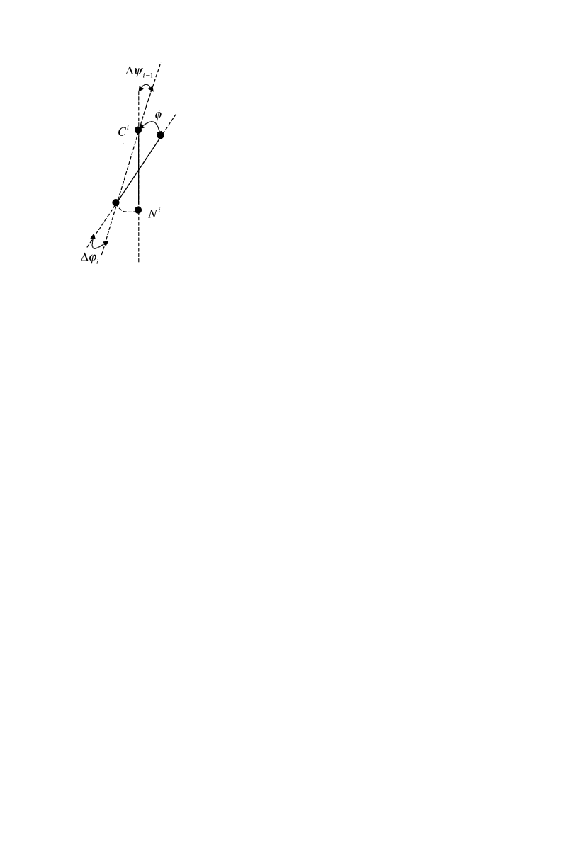
Figure 2: A look on the peptide group from the axis of rotation $\sigma$ explaining the definition of the angle $\phi$ (defined in (3)).

The rocking of the rigid plane of the peptide group (the so called ”crankshaft-like” motion) due to degrees of freedom of torsional (dihedral) angles $\varphi_{i}$ and $\psi_{i-1}$ (see Fig.1) was proposed on theoretical grounds from normal-mode analysis [37]. It is supported by numerous NMR experiments and molecular dynamics simulations of protein backbone [38], [39], [40], [41], [42], [43], [44], [45], [46], [47], [48], [49], [50], [51]. The crankshaft-like motion is comprehended now as a dominant type of motion for the protein backbone that ”involves only a localized oscillation of the plane of the peptide group” [51]. The essence of this motion is the so called anticorrelated motion of the torsional angles $\varphi_{i}$ and $\psi_{i-1}$ manifested itself in the requirement (see Fig.2)

$$\phi/2\equiv\Delta\varphi_{i}=\Delta\psi_{i-1}$$ (3)

In this case the plane of the peptide group rocks as a whole around some axis $\sigma$ that goes through the center of masses of the peptide group parallel to the bonds $C_{\alpha}^{i-1}-C^{i}$ and $N^{i}-C_{\alpha}^{i}$ (see Fig.1). The moment of inertia of the peptide group relative to the axis $\sigma$ is known to be $I\approx 7.34\cdot 10^{-39}g\cdot cm^{2}$ [52]. However this value is given in [52] without a reference or calculation. That is why in Appendix A a brief estimate corroborating this value is given. Molecular dynamics simulations and NMR experimental data testify that the character of the correlation function for the crankshaft motion is decaying oscillations [40], [51]. However they provide characteristics for them in a very wide range from the subpicosecond and picosecond time scale [51] to slower motions on a much larger time scale from tens of picoseconds to 100 ps and more [50]. This is presumably a particular manifistation for the cranckshaft motion of a general principle of hierarchical structure for a conformational potential in protein dynamics [3], [5], [11] when a group of local minima forms a smooth local minimum and so on. In fact knowing the actual values of the frequency for the oscillations and the characteristic time of their decay for the functionally important crankshaft motion is not indespesible for the purposes of the present paper. However in our opinion it is reasonable to assume that the frequency of oscillations of the plane of the peptide group as a whole for such motion should be at least order of magnitude less than those for high frequency in - plane motions such as, e.g., Amide I ($\sim 1600\ cm^{-1}$). The choice of the frequency in the $\omega_{0}\sim 100\ cm^{-1}\approx 10^{13}\ s^{-1}$ range enables us to match it with the amplitudes of rocking of order of several degrees (see (12) below) in accordance with experimental data [47], [49].

It is natural to describe the cranckshaft motion by a Langevin equation. Such equations are frequently used in protein dynamics [53], [54], [55]. The equation of the cranckshaft motion for the rigid plane of the peptide group in the above conditions is

$$I\frac{d^{2}\phi(t)}{dt^{2}}+\gamma\frac{d\phi(t)}{dt}+I\omega_{0}^{2}\phi(t)=\xi(t)$$ (4)

where $\gamma$ is the friction coefficient and $\xi(t)$ is the random torque with zero mean $<\xi(t)=0>$ and correlation function

$$<\xi(0)\xi(t)>=2k_{B}T\gamma\delta(t)$$ (5)

$k_{B}$ is the Boltzman constant, $T$ is the temperature.

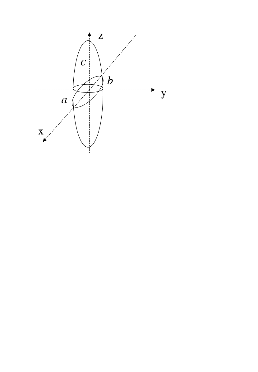
Figure 3: Model of the peptide group by oblate ellipsoid.

We consider the hydrodynamic friction. This ”macroscopic” notion is known to work surprisingly well at the molecular level (see [56] for thorough discussion). We model the peptide group by an oblate ellipsoid with halfaxes $a$, $b$ and $c$ (where $a\sim c$ and $a,c>>b$ that reflects the flat character of the peptide group) Fig. 3. For the rotation of the ellipsoid around $x$-axis (that is in our case actually the axis $\sigma$ for the peptide group introduced above) the friction coefficient is given by a formula [57]

$$(\gamma)_{x}=8\pi\eta\ abc\left[\frac{12r}{a}+\frac{(bc)^{1/4}}{a^{1/2}\left(1+\frac{4r}{a^{1/2}(bc)^{1/4}}\right)^{3}}\right]^{-1}$$ (6)

where $r=2(abc)^{1/3}$ and $\eta$ is the viscosity of the ellipsoid environment. The required behavior is obtained if we have the condition of the underdamped motion

$$\frac{\gamma}{I\omega_{0}}<<1$$ (7)

Let us meke a numerical estimate of this requirement. Taking the linear size of the peptide group (distance for the atom $O$ to the atom $H$) to be $L\approx 2.5\ \AA$ we have $c\approx L/2$, $a\approx c/2$ and $b\approx a/3$. From (6) we obtain that at $\eta\approx 1\ cP$ (that is the viscosity of water at room temperature) $\gamma\approx 2\cdot 10^{-27}\ CGS$. Then at typical value $\omega_{0}\approx 10^{13}s^{-1}$ and the value $I\approx 7.34\cdot 10^{-39}g\cdot cm^{2}$ we have $\gamma/(I\omega_{0})\approx 0.01$, i.e., the requirement (7) is by far satisfied. Moreover it well holds even at the increase of $\eta$ by an order of magnitude.

At the requirement (7) we obtain (see e.g. [58], [55])

$$\alpha(t)\equiv<\phi(0)\phi(t)>\approx\frac{k_{B}T}{I\omega_{0}^{2}}exp\left(-\frac{\gamma\mid t\mid}{2I}\right)cos\left(\omega_{0}t\right)$$ (8)

We denote

$$\mu=\frac{\gamma}{\sqrt{2}I\omega_{0}}$$ (9)

Then the Fourier spectrum for the correlation function $\alpha(t)$ is

$$\tilde{\alpha}(\omega)=\frac{k_{B}T}{I\omega_{0}^{2}}\frac{\mu}{\pi}\frac{1+\mu^{2}+\left(\omega/\omega_{0}\right)^{2}}{\mu^{4}+2\mu^{2}\left[1+\left(\omega/\omega_{0}\right)^{2}\right]+\left[1-\left(\omega/\omega_{0}\right)^{2}\right]^{2}}$$ (10)

At our requirement (7) it has a sharp resonance peak at the frequency $\omega_{0}$. For the mean squared amplitude ($msa$) we have

$$msa=\frac{k_{B}T}{I\omega_{0}^{2}}$$ (11)

The latter means that the amplitude of the cranckshaft motion at room temperature and, e.g., typical value $\omega_{0}\approx 10^{13}s^{-1}$ is

$$\phi_{max}=\sqrt{\frac{k_{B}T}{I\omega_{0}^{2}}}\approx 0.1\approx 6^{\circ}$$ (12)

that is $\Delta\varphi_{i}=\Delta\psi_{i-1}\approx 3^{\circ}$. This value sheds light on the origin of essentially vibrational character of the peptide group motion manifested itself in (8) and (10). At such angles of rotational deviation of the peptide group from its mean averaged position the linear displacements of the atoms are $\sim c\cdot\phi_{max}\approx 0.1\ \AA$. The latter value is much less than both the size of a solvent molecule and interatomic distances to neighbor fragments of protein structure. That is why the environment exerts rather weak friction for such type of the peptide group motion that is reflected in the requirement (7). Thus we conclude that the thermally equilibrium cranckshaft motion of the peptide group is of essentially vibrational character even in such condensed medium as protein interior.

3 Essence of the RPV

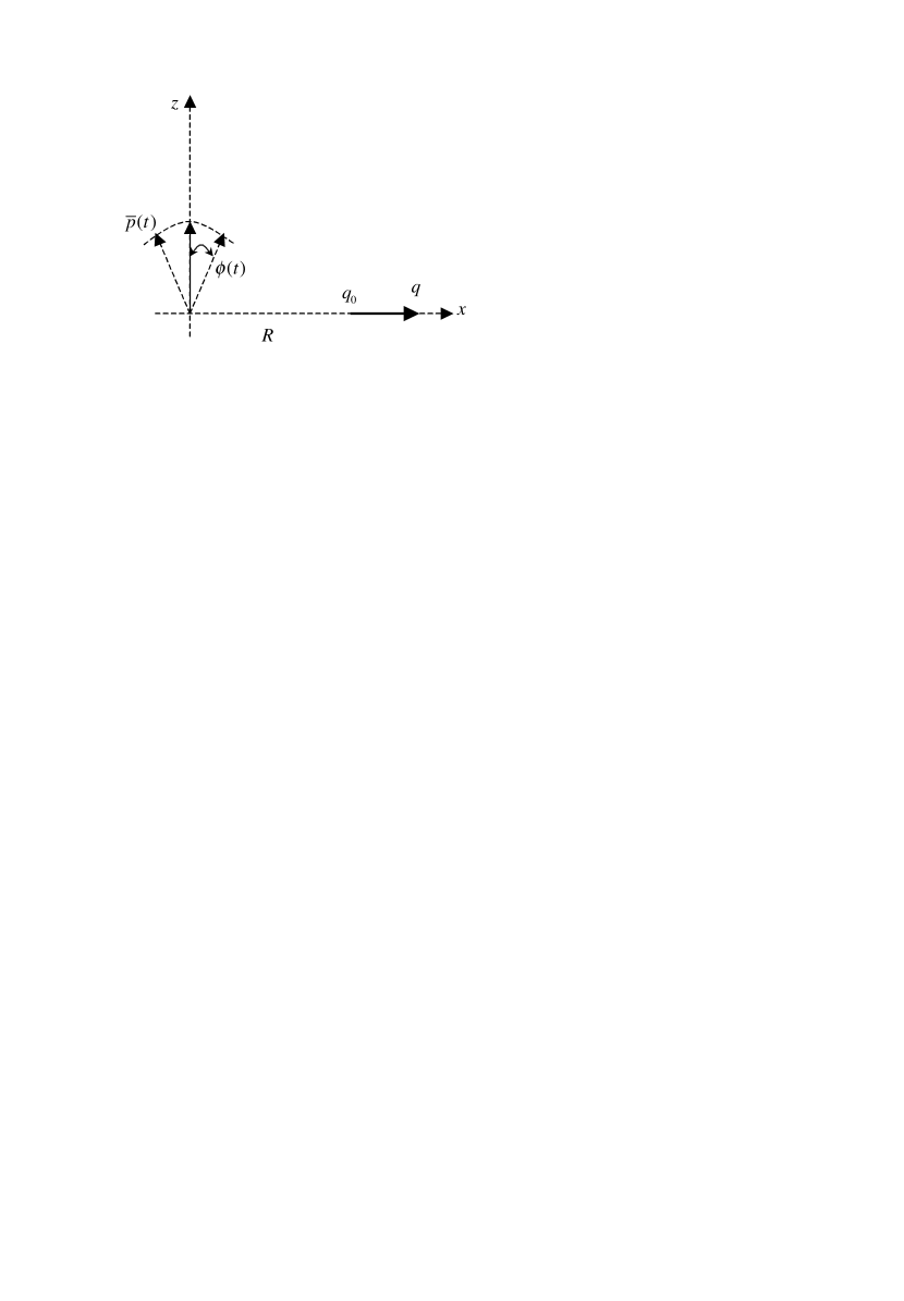
Figure 4: Favourable orientation of the peptide group dipole moment $\bar{p}(t)$ relative to the reaction coordinate $q$.

We consider the plane of the peptide group that undergoes thermally equilibrium rocking around its mean averaged position. The angle $\phi(t)$ quantifies the random deviations of the plane. We choose the axis $x$ in the direction of these deviations (see Fig.4). Now we recall that there is the dipole moment of the peptide group with the absolute value $p\approx 3.6\ D$ laying in its plane. We choose the axis $z$ in the direction of the dipole moment at the mean averaged position of the peptide group. Thus the dipole moment is a vector in our frame

$$\bar{p}(t)=p\ sin\phi(t)\ \bar{e}_{x}+p\ cos\phi(t)\ \bar{e}_{z}$$ (13)

Taking into account that $\mid\phi(t)\mid<<1$ we have

$$\bar{p}(t)\approx p\ \phi(t)\ \bar{e}_{x}+p\ \bar{e}_{z}$$ (14)

We assume a simplest geometry favorable for catalysis (generalizations are trivial but lead to more cumbersome formulas of not principle character). In this geometry at a distance $R$ from the dipole moment along the axis $x$

$$\bar{R}=R\ \bar{e}_{x}$$ (15)

there is a reaction coordinate $q$. The latter has a transition dipole moment $\bar{d}$ due to separation of charges with the value $e$ at movement along it

$$\bar{d}=e(q-q_{0})\bar{e}_{x}$$ (16)

Here $q_{0}$ is the position of the minimum of the potential energy surface corresponding to initial reagent. Then the quasistationary fluctuating electric field of the peptide group dipole moment in the place of the reaction coordinate is

$$\bar{E}(t)=\frac{3\left(\bar{p}(t)\cdot\bar{R}\right)\bar{R}-R^{2}\bar{p}(t)}{\epsilon R^{5}}\approx\frac{p}{\epsilon R^{3}}\left[2\phi(t)\bar{e}_{x}-\bar{e}_{z}\right]$$ (17)

where $\epsilon$ is the dielectric constant. Denoting

$$g=\frac{2ep}{\epsilon R^{3}}$$ (18)

we obtain for the interaction of the peptide group dipole moment with the transition dipole moment of the reaction coordinate

$$H_{int}=-\left(\bar{d}\cdot\bar{E}(t)\right)=-g(q-q_{0})\phi(t)$$ (19)

This interaction reveals the essence of the RPV as fluctuating electric field affecting the reaction coordinate.

4 Equations of motion

We denote $m$ the effective mass of the reaction coordinate $q$ and $V(q)$ the potential energy surface for it. We assume the most frequently used memory-free friction (Ohmic damping) for both the reaction coordinate and the peptide group cranckshaft motion. For the reaction coordinate it can be motivated as follows. Taking into account the memory friction (that leads to the generalized Langevin equation, e.g., in the spirit of Grote-Hynes approach) is usually necessary for fast reactions (e.g., those with low activation barriers). Enzymatic reactions typically have a rather high barrier (even after its reduction by catalytically active groups). Thus the limit of a very rapidly fluctuating force compared with the rate of the transition over the barrier (the reaction dynamics is very slow and the environment exerts its full frictional influence during barrier crossing) can be safely taken. In this case the generalized Langevin equation is well approximated by the ordinary one. For the high - frequency cranckshaft motion of the peptide group the approximation of Ohmic damping can not be logicaly motivated because the characteristics of the correlation function (inverse frequency of oscillations and decay time) are comparable with the characterisic time of surrounding rearrangements acting as thermal bath. Besides taking into account memory friction for peptide dynamics can be implemented rather easily in the approximation of harmonic conformational potential [15], [54], [59], [60], [61]. However it usually leads to complications of not principal character at room temperatures (well above the so called ”glass” transition in protein dynamics) where enzymes normally work. In this temperature range conformational protein dynamics are satisfactorily described by ordinary Langevin equation.

Then we have classical equations of motion are

$$m\ddot{q}+V^{\prime}(q)-g\phi+\nu\dot{q}=\zeta(t)$$ (20)

$$I\ddot{\phi}+I\omega^{2}_{0}\phi-g(q-q_{0})+\gamma\dot{\phi}=\xi(t)$$ (21)

where the coupling constant $g$ is given by (18). In (20) $\nu$ is the friction coefficient for translational motion along the reaction coordinate (modeled by effective Brounian particle with the caharacterisic linear size $l$ in the media with viscosity $\eta$ and given by the Stokes formula $\nu=6\pi l\eta$ (see next Sec.)) and $\zeta(t)$ is the random force characterized by

$$<\zeta(t)>=0;\ \ \ \ \ \ \ \ \ \ \ <\zeta(0)\zeta(t)>=2k_{B}T\nu\delta(t)$$ (22)

In (21) $\gamma$ is the friction coefficient for rotational fluctuations of the peptide group given by (6) and $\xi(t)$ is the random torque characterized by

$$<\xi(t)>=0;\ \ \ \ \ \ \ \ \ \ \ <\xi(0)\xi(t)>=2k_{B}T\gamma\delta(t)$$ (23)

Neglecting the ”backward” influence of the reaction coordinate on the peptide group motion (term $-g(q-q_{0})$ in (21)) we obtain for the latter the previously considered equation of motion (4) and are left with a two noise problem

$$m\ddot{q}+V^{\prime}(q)+\nu\dot{q}=\zeta(t)+g\phi(t)$$ (24)

Here the internal (its intensity is related with friction coefficient $\nu$) white noise $\zeta(t)$ is characterized by (22) and the external (it does not create friction for the movement along the reaction coordinate $q$) oscillating noise $\phi(t)$ is characterized by

$$<\phi(t)>=0;\ \ \ \alpha(t)\equiv<\phi(0)\phi(t)>\approx\frac{k_{B}T}{I\omega_{0}^{2}}exp\left(-\frac{\gamma\mid t\mid}{2I}\right)cos\left(\omega_{0}t\right)$$ (25)

The stochastic influence $g\phi(t)$ has no counterpart for reactions in solution. It is unique for enzymatic reactions because it is produced by dynamics of protein structure (namely by a favourably located and oriented peptide group in the present model or may be by a few of them in more realistic cases). In solution solvent molecules also posess dipole moments and undergo thermal motion. However they do not form strictly determined structure enabling them to implement high-frequency motion of essentially vibrational character as in the case of peptide groups in proteins.

The equations (24), (22), (25) belong to a class of the problems considered recently in [62], [63]. Regretfully the formulas obtained there lead to very cumbersome manipulations in our case and this most natural way of formulating the problem has not led to representable results for oscillating noise (25) yet. That is why we have to resort to simplifying assumptions. First of all we take into account that a reaction of bond breaking or bond making requires linear displacements of atoms of order of the bond length $\sim 1\ \AA$ that is comparable with the size of solvent molecules. Hence the solvent exerts rather strong friction for the movement of the system along the reaction coordinate. Thus we can restrict ourselves by the high friction limit, i.e., neglect the inertial term $m\ddot{q}$ in (24). The requirement for the overdamped regime is $\nu/(m\omega_{b})>>1$ where the friction coefficient is given by the Stokes formula $\nu=6\pi l\eta$ (see next Sec.) and the frequency $\omega_{b}$ characterizes the shape of the potential barrier at its top $\omega_{b}=\sqrt{\mid V^{\prime\prime}(q_{b})\mid/m}$. At $l\approx 1\ \AA$ and $\eta\approx 1\ cP$ (that is the viscosity of water at room temperature) we have the estimate $\nu\approx 2\cdot 10^{-9}\ CGS$. Then at typical values $\omega_{b}\sim 10^{3}\ cm^{-1}\approx 10^{14}\ s^{-1}$ and $m\approx 5\ a.u.m.$ ($a.u.m.\approx 1.7\cdot 10^{-24}g$) we obtain $\nu/(m\omega_{b})\approx 2$. Thus the requirement of overdamped regime does not hold well in pure solvent but becomes satisfactory with the increase of viscosity. A generalization of the theory with taking into account the inertial term in the ordinary Langevin equation is indispensable for the description of reactions in a gas phase that proceed in the underdamped limit. Those in condensed media (in solution or in an enzyme) are generally believed to proceed typically in the overdamped regime and we also resort to this assumption for simplification of further analysis. We stress once more the reason why for the motion of the peptide group we apply the underdamped regime while for the movement along the reaction coordinate we invoke to the overdamped one. In the former case the linear displacements of the atoms are $\approx 0.1\ \AA$, i.e., much less than the size of the solvent molecules $\approx 1\ \AA$ (see Sec. 2). In the latter case the linear displacements of atoms are comparable with the size of the solvent molecules. That is why the friction is supposed to be sufficiently strong for the overdamped regime to be applicable.

Most important of all we resort to a severe approximation based on the following reasoning. Strictly speaking a Fourier mode of the random process $\phi(t)$

$$\tilde{\phi}(\omega)=\frac{1}{2\pi}\int_{-\infty}^{\infty}dt\ \phi(t)exp(-i\omega t)$$ (26)

is a random function of frequency with zero mean. However the mean squared amplitude of this mode is related to the correlation function $\alpha(t)$ via the Wiener-Khinchin theorem

$$<\mid\tilde{\phi}(\omega)\mid^{2}>=\int_{-\infty}^{\infty}dt\ \alpha(t)exp(-i\omega t)=2\pi\tilde{\alpha}(\omega)$$ (27)

where $\tilde{\alpha}(\omega)$ is given by (10). We can introduce the effective mean amplitude at any frequency as the square root of (27). In particular we can do it for the frequency $\omega_{0}$

$$<\mid\tilde{\phi}(\omega_{0})\mid>_{eff}=\sqrt{2\pi\tilde{\alpha}(\omega_{0})}$$ (28)

As was already mentioned after (10) the spectrum of $\alpha(\omega)$ at the requirement (7) has a sharp resonant peak at the frequency $\omega_{0}$. It means that practically the whole power of the spectrum is in the Fourier mode $\tilde{\phi}(\omega_{0})$ of the random process $\phi(t)$ at this frequency. That is why we can roughly approximate the random process $\phi(t)$ by a harmonic vibration with the amplitude given by (28)

$$\phi(t)\approx<\mid\tilde{\phi}(\omega_{0})\mid>_{eff}\ sin(\omega_{0}t)$$ (29)

From (9), (10) with taking into account (7) we obtain

$$\phi(t)\approx\sqrt{\frac{\sqrt{2}k_{B}T}{\gamma\omega_{0}}}\ sin(\omega_{0}t)$$ (30)

This artificial replacement of the oscillating noise (that is a random process with the properties (25)) by oscillations (30) simplifies the problem significantly and enables us to employ some known results from the Kramers’ theory. As was stressed above it is a methodical trick enabling us to cast the problem into a tractable form rather than an indespensable assumption for our approach.

5 Effect of the RPV

A standard tool to investigate dynamical effects in reaction rate is the Kramers’ theory (for review see [20], [64], [65], [66] and refs. therein). The latter is based on the ordinary Langevin equation of motion along the reaction coordinate $q$. In the Kramers’ theory a chemical reaction is modeled as the escape of a Brownian particle with the mass $m$ (the effective mass of the reaction coordinate, e.g., the reduced mass of a scissile bond) and linear size $l$ in the media with viscosity $\eta$ (so that the friction coefficient is given by the Stokes formula $\nu=6\pi l\eta$) and temperature $T$ from the well of a metastable potential along the reaction coordinate. This potential is an electronically adiabatic ground state obtained in the Born-Oppenhaimer approximation by methods of quantum chemistry. It is considered as preliminary input information for the Kramers’ theory and neither its origin nor its possible modification by catalysts is an issue of the present approach.

For the potential $V(q)$ we consider an arbitrary form with a barrier that has at the top of the latter the value $V^{\prime\prime}(q_{b})\approx-m\omega^{2}_{b}$ and at the bottom of the well the value $V^{\prime\prime}(q_{a})\approx m\omega^{2}_{a}$. Also we include into consideration the oscillating force

$$g\phi(t)=h\ sin(\omega_{0}t)$$ (31)

where

$$h=\frac{2ep}{\epsilon R^{3}}\sqrt{\frac{\sqrt{2}k_{B}T}{\gamma\omega_{0}}}$$ (32)

As a result the ordinary Langevin equation of motion along the reaction coordinate $q$ (24) takes the form

$$\nu\frac{dq}{dt}=-V^{\prime}(q)+h\ sin(\omega_{0}t)+\zeta(t)$$ (33)

We introduce the dimensionless variables and parameters as follows

$$q\rightarrow q(q_{b}-q_{a});\ \ \ \ \ t\rightarrow t\frac{\nu}{m\omega^{2}_{b}};\ \ \ \ \ \omega_{0}\rightarrow\frac{\omega_{0}\nu}{m\omega^{2}_{b}}=\Omega$$ (34)

and denote

$$A=\frac{h}{m\omega^{2}_{b}(q_{b}-q_{a})};\ \ \ \ \ D=\frac{k_{B}T}{m\omega^{2}_{b}(q_{b}-q_{a})^{2}}$$ (35)

where $A$ is the dimensionless parameter characterizing the oscillating electric field strength and $D$ is the dimensionless parameter characterizing the intensity of thermal fluctuations (i.e., the temperature of the heat bath) relative to the barrier height. Their ratio is the most important parameter of the model

$$\frac{A}{D}=\frac{h(q_{b}-q_{a})}{k_{B}T}=\frac{2ep(q_{b}-q_{a})}{\epsilon R^{3}}\sqrt{\frac{\sqrt{2}}{\gamma\omega_{0}k_{B}T}}$$ (36)

In dimentionless variables the Langevin equation is

$$\frac{dq}{dt}=-U^{\prime}(q)+Asin(\Omega t)+\chi(t)$$ (37)

where $U(q)$ is the dimensionless potential and the dimensionless noise $\chi(t)=\frac{1}{m\omega_{b}^{2}(q_{b}-q_{a})}\zeta\left(\frac{t\nu}{m\omega_{b}^{2}}\right)$ is characterized by $<\chi(t)>=0$ and $<\chi(0)\chi(t)>=2D\delta(t)$. The corresponding overdamped limit of the Fokker-Planck equation for the probability distribution function $P(q,t)$ [20] is

$$\frac{\partial P(q,t)}{\partial t}=-\frac{\partial}{\partial q}\Bigl{\{}[-U^{\prime}(q)+Asin(\Omega t)]P(q,t)\Bigr{\}}+D\frac{\partial^{2}P(q,t)}{\partial q^{2}}$$ (38)

In the absence of driving ($A=0$) the escape rate is given by the famous Kramers’ formula

$$\Gamma_{K}\approx\frac{\omega_{a}\omega_{b}}{2\pi}exp\Bigl{[}-\Bigl{(}U(q_{b})-U(q_{a})\Bigr{)}/D\Bigr{]}$$ (39)

where $\omega_{a}=\sqrt{U^{\prime\prime}(q_{a})}$ and $\omega_{b}=\sqrt{|U^{\prime\prime}(q_{b})|}$. In the case of thermally activated escape with periodic driving ($A\not=0$) one usually introduces the instantaneous rate constant $\Gamma(t)$, the rate constant $\overline{\Gamma}$ averaged over the period of oscillations $T=2\pi/\Omega$ and is interested in the escape rate enhancement $\overline{\Gamma}/\Gamma_{K}$ (see [64], [67], [68], [69] and refs. therein). Regretfully no workable formula for the general case of arbitrary modulation amplitude to noise intensity ratio $A/D$ and arbitrary frequency $\Omega$ is available at present. However the case of moderately weak to moderately strong modulation $D<<A<<\sqrt{D}$ is relevant for our problem. In this case a simple formula for the escape rate enhancement is known [68]

$$\Delta\equiv\frac{\overline{\Gamma}}{\Gamma_{K}}\approx\frac{\sqrt{D}}{\sqrt{2\pi Ac\left(\Omega\right)\left(1+O(A)\right)}}exp\Biggl{[}\frac{Ac\left(\Omega\right)}{D}\left(1+O(A)\right)\Biggr{]}$$ (40)

where for the cubic (metastable) potential $c\left(\Omega\right)=\pi\Omega/sh\left(\pi\Omega\right)$ and for the quartic (bistable) potential $c\left(\Omega\right)=\sqrt{\pi\Omega/sh\left(\pi\Omega\right)}$. This formula is sufficient for the purposes of the present paper to understand the solvent viscosity dependence in the preexponent. However it should be stressed that it is invalid is one wish to evaluate reaction rate enhancement due to the suggested mechanism. In this case the corrections $O(A)$ lead to deviation from the log-linear behavior predicted by (40). Fortunatly the latter problem is not a matter of the present paper and (40) suffices for our needs. However we briefly return to the problem of evaluation of the reaction rate enhancement due to the suggested mechanism in the next Sec. and in Appendix B.

6 Numerical estimates

Before proceed further we should define the range of the parameters for our model. To be supported by evidence we take the numerals for a very typical and one of the most studied enzymatic reaction catalysed by Subtilisin. This enzyme belongs to serine proteases and brakes the bond between the atoms C and N in a peptide group of a substrate of protein nature. At physiological temperatures where enzymes normally work ($k_{B}T\approx 4.2\cdot 10^{-14}\ CGS$) the corresponding noncatalysed reaction in solution typically has the rate constant $k\approx 1\cdot 10^{-8}\ s^{-1}$ while the enzymatic reaction has the rate constant (that of the rate limiting step) $k_{cat}\approx 5\cdot 10^{1}\ s^{-1}$ [70]. Thus the total catalytic effect is approximately $10^{12}$. We have for the friction coefficient of the movement along the reaction coordinate $\nu=6\pi l\eta$ at $l\approx 1\ \AA$ and $\eta\approx 1\ cP$ (that is the viscosity of water at room temperature) the estimate $\nu\approx 2\cdot 10^{-9}\ CGS$. Then taking into account that we measure dimensionless time in the units of $\frac{\nu}{m\omega^{2}_{b}}$ (see (34)) we have for the reaction rate constant of the noncatalysed reaction in dimensionless form at $m\approx 5\ a.u.m.$ ($a.u.m.\approx 1.7\cdot 10^{-24}g$) and $\omega_{b}\approx 10^{14}s^{-1}$ the value $\Gamma=\frac{k\nu}{m\omega_{b}^{2}}\approx 10^{-22}$. We can evaluate from the Arrhenius factor of the Kramers’ rate in the dimensionless form for the quartic (bistable) potential $V(q)=-q^{2}/2+q^{4}/4$ [20]

$$\Gamma_{K}=(\sqrt{2}\pi)^{-1}exp\biggl{[}-1/(4D)\biggr{]}$$ (41)

that in order to obtain such a reaction rate constant in the absence of the oscillating electric field ($A=0$) we should take $D\approx\frac{1}{4\cdot 22\ ln10}\approx 5\cdot 10^{-3}$. If we take the cubic (metastable) potential $V(q)=q^{2}/2-q^{3}/3$ then we obtain $D\approx 3\cdot 10^{-3}$. Thus the typical noise intensity for enzymological problems is

$$D\approx 3\div 5\cdot 10^{-3}$$ (42)

As earlier we assume that the dimensional frequency of the RPV is on the picosecond time scale and is approximately $\omega_{0}\approx 100\ cm^{-1}\approx 10^{13}\ s^{-1}$. Then from (34) we obtain at $m\approx 5\ a.u.m.$ and $\omega_{b}\approx 10^{14}\ s^{-1}$ that the dimensionless frequency in our case is

$$\Omega\approx 2\cdot 10^{-1}<<1$$ (43)

Thus we are actually in the low frequency regime or that of slow modulation $\Omega<<1$. In this case we have $c\left(\Omega\right)\approx 1$ for both cubic (metastable) and quartic (bistable) potentials. That is why $c\left(\Omega\right)$ will be droped further from the formula for the reaction rate enhancement.

We take the value $p=3.6\ D$ and typical values: for the partial charge $e\approx 0.3\ a.u.c.$ ($a.u.c.=4.8\cdot 10^{-10}\ CGS$), for the reaction potential $q_{b}-q_{a}\approx 1\ \AA$, for the dielectric constant in protein interior $\epsilon\approx 3.5$, for the distance of the fluctuating peptide group from the reaction coordinate $R\approx 3\ \AA$, for the frequency of the RPV $\omega_{0}\approx 100\ cm^{-1}\approx 10^{13}\ s^{-1}$ and for the friction coefficient of the peptide group (see Sec.2) $\gamma\approx 2\cdot 10^{-27}\ CGS$. Then at room temperature we obtain from (36) that $A/D\approx 10$. At such value of this parameter the formula (40) predicts the reaction rate enhancement by $3\div 4$ orders of magnitude ($log\ \Delta\approx 3.4$). This estimate requires comments. As was stressed above the formula (40) overestimates the reaction rate enhancement. As a matter of fact the corrections $O(A)$ lead to some more moderate growth than the log-linear one [67], [68], [69]. However the results presented in these papers testify that an appreciable deviation from the log-linear behavior begins at significantly higher values of modulation amplitude to noise intensity ratio $A/D$ than $A/D\approx 10$. That is why the reaction rate enhancement by $\approx 3\div 4$ orders of magnitude at $A/D\approx 10$ due to the suggested mechanism seems to be quite feasible. Here we restrain ourselves from further discussing this mostly important issue because the present paper is devoted to a particular effect manifesting itself in the preexponent rather than in the exponent of the formula (40). However in Appendix B we return to this problem and discuss it in more details.

7 Solvent viscosity effect

Returning to dimensional parameters, substituting (36) and (39) into (40) and dropping $c\left(\Omega\right)\approx 1$ (see previous Sec.) we obtain for the reaction rate constant

$$\bar{\Gamma}=\Gamma_{K}\Delta\approx\frac{m\sqrt{V^{\prime\prime}(q_{a})|V^{\prime\prime}(q_{b})|}}{2\pi\nu}exp\left[-\frac{\Bigl{(}V(q_{b})-V(q_{a})\Bigr{)}}{k_{B}T}\right]\times$$

$$\sqrt{\frac{\epsilon R^{3}}{4\pi ep(q_{b}-q_{a})}\sqrt{\frac{\gamma\omega_{0}k_{B}T}{\sqrt{2}}}}exp\Biggl{[}\frac{2ep(q_{b}-q_{a})}{\epsilon R^{3}}\sqrt{\frac{\sqrt{2}}{\gamma\omega_{0}k_{B}T}}\Biggr{]}$$ (44)

First we consider the hypothetical ”ideal” cosolvent with infinitely small molecular weight (cosolvent molecules freely penetrate into enzyme and are distributed there homogeneously). Taking into account that in this case we have both $\nu\propto\eta$ ($\nu=6\pi l\eta$) and $\gamma\propto\eta$ (see (6)) we obtain

$$\bar{\Gamma}\propto\frac{1}{\eta^{0.75}}$$ (45)

Thus the present approach yields the limit value $\beta_{max}=0.75$ for the ”ideal” cosolvent that is rather close to the extrapolated limit value $\beta_{max}\approx 0.79$ from the paper [8]. The dependence on $\eta$ in the second exponent is strongly overshadowed by the first exponent because typically we have

$$B=\frac{V(q_{b})-V(q_{a})}{k_{B}T}>>b=\frac{2ep(q_{b}-q_{a})}{\epsilon R^{3}}\sqrt{\frac{\sqrt{2}}{6\pi l\omega_{0}k_{B}T}}$$ (46)

Then in the $ln$ of the reaction rate constant $ln\ \bar{\Gamma}=const-0.75\ ln\ \eta+B-b/\sqrt{\eta}$ the last term is negligible provided the requirement (46) is satisfied.

In the $log\ \bar{\Gamma}$ vs. $log\ \eta$ coordinates the formula (44) yields the lines that resemble the behavior of the straight ones from the paper [8]. To exhibit it explicitly let us return to dimensionless variables and parameters and write $\eta=\eta_{0}\ 10^{x}$ where $\eta_{0}=1\ cP$ at which we typically have $\left(A/D\right)_{0}\approx 10$ (see previous Sec.). Then we obtain

$$log\ \bar{\Gamma}=log\left[\frac{\omega_{a}\omega_{b}}{2\pi}\sqrt{\frac{1}{2\pi}\left(\frac{D}{A}\right)_{0}}\right]-\frac{log\ e}{nD}-\frac{3x}{4}+\left(\frac{A}{D}\right)_{0}\ \frac{log\ e}{10^{x/2}}$$ (47)

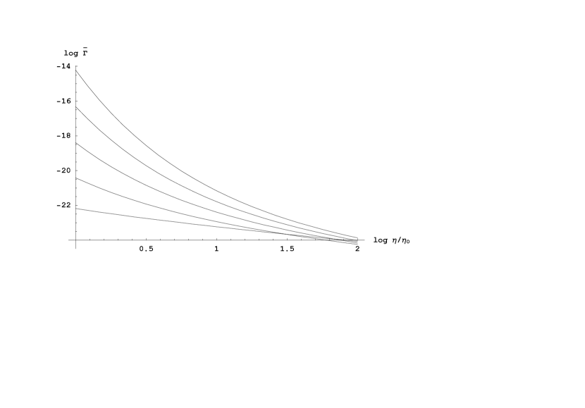
Figure 5: Dependence of the reaction rate constant $\bar{\Gamma}$ on solvent viscosity $\eta$ in the $log\ \bar{\Gamma}$ vs. $log\ \left(\eta/\eta_{0}\right)$ coordinates given by formula (47) for the case of quartic (bistable) potential. The values of $\left(A/D\right)_{0}$ from the down line to the upper one respectively are: 1, 6, 11, 16, 21.

where for the cubic (metastable) potential $\omega_{a}=1$, $\omega_{b}=1$ and $n=6$ while for the quartic (bistable) potential $\omega_{a}=\sqrt{2}$, $\omega_{b}=1$ and $n=4$. The plots for the latter case obtained with the help of the formula (47) are depicted in Fig.5. However we should recognize that the lines obtained are in bad accordance with the results of the paper [8]. At realistic values $A/D\approx 10$ we obtain too large decrease of the reaction rate constant $\approx 6$ orders of magnitude instead of $\approx 1$ order of magnitude in [8] at the increase of solvent viscosity by $2$ orders of magnitude. Besides the lines for this case deviate appreciably from the straight ones obtained in [8]. That is why in Appendix B we return to this problem and show that taking into account the corrections $O(A)$ to the formula (40) for the reaction rate enhancement improves the situation significantly and yields the results that are in good agreement with experimental data from the paper [8].

Now we consider a realistic cosolvent with finite molecular weight $M$. In this case both friction coefficients $\nu$ and $\gamma$ are some unknown functions of solvent viscosity. The cosolvent molecules with larger molecular weight worser penetrate both into the enzyme active site where the reaction coordinate is located and into the enzyme body where the functionally important cranckshaft-like motion of favourably located peptide groups takes place. That is why with the increase of $M$ these functions should grow more slowly the higher the $M$ is. Thus cosolvent molecules with larger molecular weight should create less pronounced dependence on solvent viscosity than those with lesser molecular weight. In our opinion there are not enough experimental data to define these functions reliably on physical grounds. That is why we further resort to speculations of purely phenomenological character. We assume that these functions are of the form $\nu\propto\eta^{\delta(M)}$ and $\gamma\propto\eta^{\alpha(M)}$ with the requiremens that the indecies of a power $\delta(M)$ and $\alpha(M)$ obey $\lim_{M\to 0}{\delta(M)}=1$, $\lim_{M\to 0}{\alpha(M)}=1$ and are decaying functions with the increase of $M$. These requirements take into account the above mentioned features.

Then the formula (44) yields

$$\bar{\Gamma}\propto\frac{1}{\eta^{\beta(M)}}$$ (48)

where

$$\beta(M)=\delta(M)-\frac{\alpha(M)}{4}$$ (49)

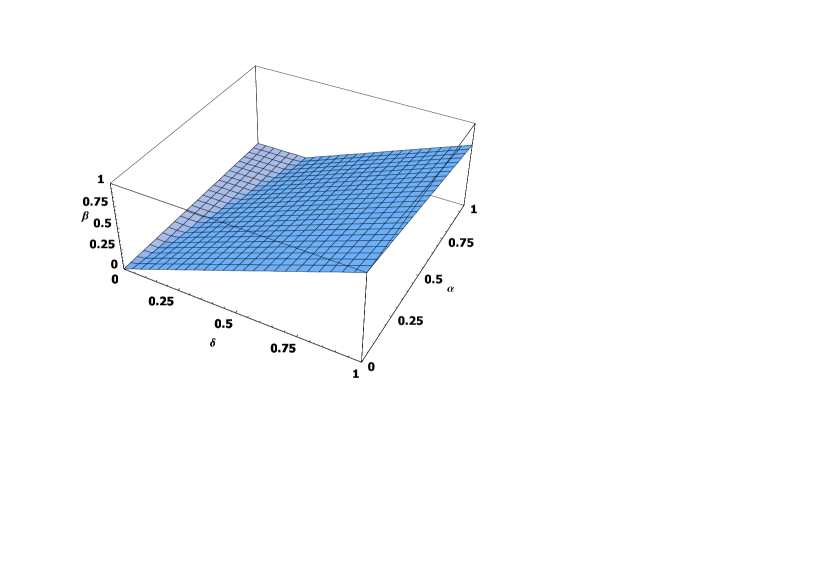
Figure 6: Dependence of the parameter $\beta=\delta-\alpha/4$ (see (48)) on the values of $\delta$ and $\alpha$.

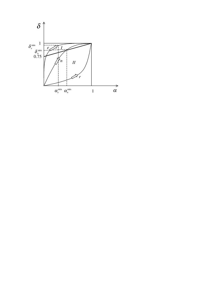
Figure 7: Three types of possible behavior of the parameters $\delta(M)$ and $\alpha(M)$ on cosolvent molecular weight $M$: $n$-normal, $r$-rare and $e$-exceptional. The fat line devides the parameter space to the region $I$ where $\beta=\delta-\alpha/4>0.75$ and the region $II$ where $\beta=\delta-\alpha/4<0.75$.

Regretfully the experimental data available for $\beta(M)$ do not allow us to distinguish $\delta(M)$ and $\alpha(M)$ separately. We can only say that from the requirement $\beta(M)>0$ we should have $\delta(M)>\alpha(M)/4$. The dependence of the parameter $\beta$ on the values of $\delta$ and $\alpha$ is presented in Fig. 6. One can distinguish two regions (see also Fig. 7): in the region $I$ we have $\beta>0.75$ while in the region $II$ we have $\beta<0.75$. Accordingly three possible types of behavior are concievable. We call them normal, rare and exceptional and schematically depict in Fig.7. Let us start from the case of large cosolvent molecular weight when both $\delta(M)$ and $\alpha(M)$ are small. For the rare type of behavior the decrease of $M$ leads to a path in the $\alpha-\delta$ parameter space that is always left in the region $I$, i.e., the value $\beta(M)$ is always less than the limit value $\beta_{max}=0.75$. For the normal type of behavior the path crosses the fat line and enters the region $II$ where $\beta(M)>0.75$. At the minimal realistic cosolvent molecular weight $M=62$ for Ethylenglycol (see [8]) we have some $\alpha_{n}^{min}$ and $\delta_{n}^{min}$ at which we generally can obtain arbitrary $0.75<\beta_{max}<1$. Finally for the exceptional type of behavior we can obtain $\alpha_{e}^{min}$ so small and $\delta_{e}^{min}$ so large that $\beta_{max}=\delta_{e}^{min}-\alpha_{e}^{min}/4\approx 1$, i.e., the approximate dependence $\bar{\Gamma}\propto 1/\eta$ emerges.

Also the formula (44) yields the dependence of the reaction rate constant on dielectric constant $\epsilon$. Such dependence has been known from the experiment for a long time [1] and is of the type $ln\ k_{cat}=...+const/\epsilon$. The formula (44) predicts $ln\ \bar{\Gamma}=...+const/\epsilon+(1/2)ln\ \epsilon$. It is obvious that the latter term is practically unnoticeable on the background of the former one. That is why one can conclude that the formula (44) yields correct dependence on dielectric constant in accordance with experimental data from [1].

8 Conclusions

We suggest a dynamical mechanism that mediates the influence of solvent viscosity on the reaction coordinate at enzyme action. The mechanism is based on the fluctuations of the electric field in the enzyme active site. These fluctuations are produced by thermally equilibrium dynamics of protein structure, namely by rocking of the rigid plane of a favourably located and oriented peptide group (or may be a few of them). Such rocking causes the electric field of the dipole moment of the peptide group lying in its plane to undergo fluctuations in time. As the latter are thermally equilibrium they exist on the whole time scale of enzyme turnover and there is no problem to match them with the catalytic act. Namely the impossibility of survival for artificially constructed coherent oscillatory excitations in protein dynamics on the time scale of the catalytic act plagues many of the suggestions for dynamical contribution into enzyme action and causes justifiedly criticism of Warshel and coauthors [31], [32], [33]. Such excitations may really be created by energy released at substrate binding by an enzyme. They can exist for some life time in the form of, e.g., the so called discrete breathers either in protein highly regular secondary structure [35], [71] or in its whole irregular tertiary structure [72]. However a protein is condensed media and any motion both in its interior and on its surface of thermally nonequilibrium characher must fade away rapidly (on the enzyme turnover time scale) due to dissipation. Long life times for discrete breathers obtained in [72] are due to unphysical assumption of friction for only surface elements of the three-dimensional network of oscillators. In our opinion the only possibility is to obtain some kind of influence on the reaction coordinate (having no counterpart for reactions in solution) from thermally equilibrium fluctuations. The structure of the protein enables peptide groups to implement high frequency thermally equilibrium rocking of their rigid planes (cranckshaft motion). This is a rotational motion and linear displacements of the atoms at it are negligibly small compared with both the size of the solvent molecules and the interatomic distances in protein. That is why this type of motion proceeds in the underdamped regime even in the condensed media of protein interior and mimics oscillations very much.

The specific Fourier mode of the electric field fluctuations at some own frequency of rocking of the rigid plane of the peptide group (presumably $\omega_{0}\sim 100\ cm^{-1}$) resembles coherent oscillation and can be approximated by a harmonic vibration. The latter is the RPV in our approach. The rocking of the rigid plane of the peptide group feels the microviscosity of the environment in the vicinity of the latter. This microviscosity is a function of solvent viscosity. Details of this function depend on the molecular weight of the cosolvent very much. For the hypothetical ”ideal” cosolvent with infinitely small molecular weight (cosolvent molecules freely penetrate into enzyme and are distributed there homogeneously) the microviscosity is identical to solvent viscosity. For realistic cosolvent their relationship is more complicated and poorly known.

The mechanism suggested in the present paper yields the required functional dependence (1) of an enzymatic reaction rate constant on solvent viscosity and the limit value $\beta_{max}\approx 0.75$ that is in good agreement with the extrapolated one $\beta_{max}\approx 0.79$ from the paper [8] (see Introduction). We have considered predominantly the limiting case of the hypothetical ”ideal” cosolvent. To take into account the realistic molecular weight of the cosolvent one needs to know how its molecules are located in the enzyme both relative to the reaction coordinate and the rocking peptide group (or a few of them) interacting with the latter via electric field fluctuations. In this case both the friction coefficient for the reaction coordinate $\nu$ and that for the rocking peptide group $\gamma$ become more complicated functions of solvent viscosity $\eta$ than simple proportionality. All the arguments from the papers [1], [2], [15], [22], [23], [8], [17], [10] remain pertinent for this case. However we do not feel that there are enough data at present to tackle realistic cosolvent within our approach at a deeper level than purely phenomenological speculations. We are merely convinced that it should be done not within the Kramers’ formula yielding $k_{cat}\propto 1/\eta$ dependence but within a formula of the type of (44) where the upper limit $\beta_{max}$ is already built-in, i.e., the dependence $k_{cat}\propto 1/\eta^{\beta}$ with $\beta\leq\beta_{max}$ is obtained automatically.

Regretfully at present we have to work with very limited tools from the Kramers’ theory. The most natural formulation of our problem leads to a two noises model one of which is the oscillating noise (25). There are no results for such model in the literature yet. Further development of the model will inevitably require its elaboration within the approach of the papers [62], [63]. At present stage we have to resort to artificial approximating the oscillating noise by coherent oscillations. However even for the latter simplified case the theory of the Fokker-Planck equation (38) does not provide us at present with a workable formula for the general set of the parameters $A$, $D$ and $\Omega$. This fact does not enable us to evaluate reliably ”how much can the electric field fluctuations in the enzyme active site contribute into the reaction rate enhancement ?” because small corrections in the exponent can lead to drastic overestimations. However we argue that the low frequency regime is relevant for enzymological problems. For this case the corrections $O(A)$ to the formula (40) can be obtained explicitly (see Appendix B). They allow us conclude that the reaction rate enhancement by the suggested mechanism up to $\approx 3\div 4$ orders of magnitude is feasible. We argue that available results enable us to consider the preexponent quite safely. As the functional dependence (1) of an enzymatic reaction rate constant on solvent viscosity manifests itself namely in the preexponent the employed formula (40) seems to be sufficient for the purposes of the present paper. The discrepansies with experimental data are eliminated by taking into account the corrections $O(A)$ to this formula as the results from Appendix B testify.

We conclude that the present approach grasps the main feature of the functional dependence (1) for enzymatic reaction rate constant on solvent viscosity and satisfactorily yields the upper limit for the fractional index of a power in it.

9 Appendix A

Here we give a brief estimate of the moment of inertia of the peptide group for rotation around the axis $\sigma$ that goes through the center of masses of the peptide group parallel to the bonds $C_{\alpha}^{i-1}-C^{i}$ and $N^{i}-C_{\alpha}^{i}$ (see Fig.1). The peptide group is a rigid plane structure so that all atoms $O$, $C$, $N$ and $H$ lie in a plane. That is why the moment of inertia is simply the sum of their masses multiplied by the square of their distances to the axis $\sigma$. The masses in atomic units ($1\ a.u.m.=1.7\cdot 10^{-24}g$) are $m_{O}=16$, $m_{C}=12$, $m_{N}=14$ and $m_{H}=1$. That is why the center of masses is shifted a little to the atoms $C$ and $O$ relative the middle of the bond $C-N$. The lengths of the bonds are $l_{OC}=1.24\ \AA$, $l_{CN}=1.32\ \AA$ and $l_{NH}=1.\ \AA$. That is why the distances to the axis $\sigma$ are approximately $r_{O}\approx 1.5\ \AA$, $r_{C}\approx 0.3\ \AA$ and $r_{N}\approx 0.7\ \AA$ and $r_{H}\approx 2\ \AA$. Substituting these values into the formula $I=\sum m_{i}r_{i}^{2}$ we obtain $I\approx 7.6\cdot 10^{-39}g\cdot cm^{2}$. Thus our rough estimate corroborate the precise value $I\approx 7.34\cdot 10^{-39}g\cdot cm^{2}$ from [52].

10 Appendix B

We consider the low frequency regime $\Omega<<1$ that is argued in Sec. 6 to be relevant for our problem. For the particular case of moderately strong modulation $A<<A_{c}$ (where the bifurcational point $A_{c}$ has the values $A_{c}=0.25$ for the case of the cubic (metastable) potential $U(q)=q^{2}/2-q^{3}/3$ and $A_{c}=2/(3\sqrt{3})\approx 0.4$ for the case of the quartic (bistable) potential $U(q)=-q^{2}/2+q^{4}/4$) the reaction rate enhancement is obtained in [73]. The formula obtained there is rather cumbersom and is not presented here to save room. The results obtained with its help for the case of quartic (bistable) potential are depicted in Fig.8. They testify that at our values $D=5\cdot 10^{-3}$ and $A/D\approx 10$ (see Sec. 6) the reaction rate enhancement is $\sim 3\div 4$ orders of magnitude. Thus the conclusion that the suggested mechanism is strong enough to affect enzyme action appreciably is justified. For the intermediate regime of moderately weak to moderately strong modulation $D<<A<<\sqrt{D}$ (our estimate $A/D\approx 10$ is within this range for practically important for enzymology range $D\approx 3\div 5\cdot 10^{-3}$ (42)) the formula is simplified significantly and yields an explicit expression for the corrections $O(A)$ to the formula (40). We denote

$$p=1+\frac{2}{\omega_{b}^{2}}\Biggl{[}\frac{\omega_{a}^{2}}{4}+\frac{\pi-2}{\pi}\Biggl{(}\frac{1}{2\omega_{b}}-\frac{1}{\pi}\Biggr{)}\Biggr{]}$$ (50)

where for the cubic (metastable) potential (CP) $\omega_{a}=\sqrt{U^{\prime\prime}(q_{a})}=1$, $\omega_{b}=\sqrt{U^{\prime\prime}(q_{b})}=1$ and $q_{a}=0$, $q_{b}=1$ while for the quartic (bistable) potential (QP) $\omega_{a}=\sqrt{U^{\prime\prime}(q_{a})}=\sqrt{2}$, $\omega_{b}=\sqrt{U^{\prime\prime}(q_{b})}=1$ and $q_{a}=-1$, $q_{b}=0$.

Then we have a simple formula for the reaction rate enhancenment

$$\Delta\approx\frac{\sqrt{D}}{2\sqrt{\pi A\Bigl{[}\left(q_{b}-q_{a}\right)/2-Ap\Bigr{]}}}exp\Biggl{\{}\frac{A}{D}\Bigl{[}q_{b}-q_{a}-Ap\Bigr{]}\Biggr{\}}$$ (51)

where $p$ is the constant given by (50). For the case of CP we have $p\approx 1.632$ while for the QP we have $p\approx 2.132$. For both of them we have $q_{b}-q_{a}=1$.

From (51) we obtain a modification of the formula (47)

$$log\ \bar{\Gamma}=log\left[\frac{\omega_{a}\omega_{b}}{2\pi}\right]+log\left[\frac{1}{2\sqrt{\pi}}\sqrt{\left(\frac{D}{A}\right)_{0}}\right]-\frac{log\ e}{nD}-\frac{3x}{4}-$$

$$\frac{1}{2}log\left[\frac{1}{2}-pD\left(\frac{A}{D}\right)_{0}\ \frac{log\ e}{10^{x/2}}\right]+\left(\frac{A}{D}\right)_{0}\ \frac{log\ e}{10^{x/2}}\left[1-pD\left(\frac{A}{D}\right)_{0}\ \frac{log\ e}{10^{x/2}}\right]$$ (52)

The results obtained with the help of this formula for the case of quartic (bistable) potential ($\omega_{a}=\sqrt{2}$, $\omega_{b}=1$ and $n=4$) are depicted in Fig. 9. They are good agreement with the results of the paper [8] because they yield straight lines for the decrease of the rate constants by approximately one order of magnitude at the increase of solvent viscosity by two orders of magnitude.

Acknowledgements. The author is grateful to Dr. Yu.F. Zuev for helpful discussions. The work was supported by the grant from RFBR.

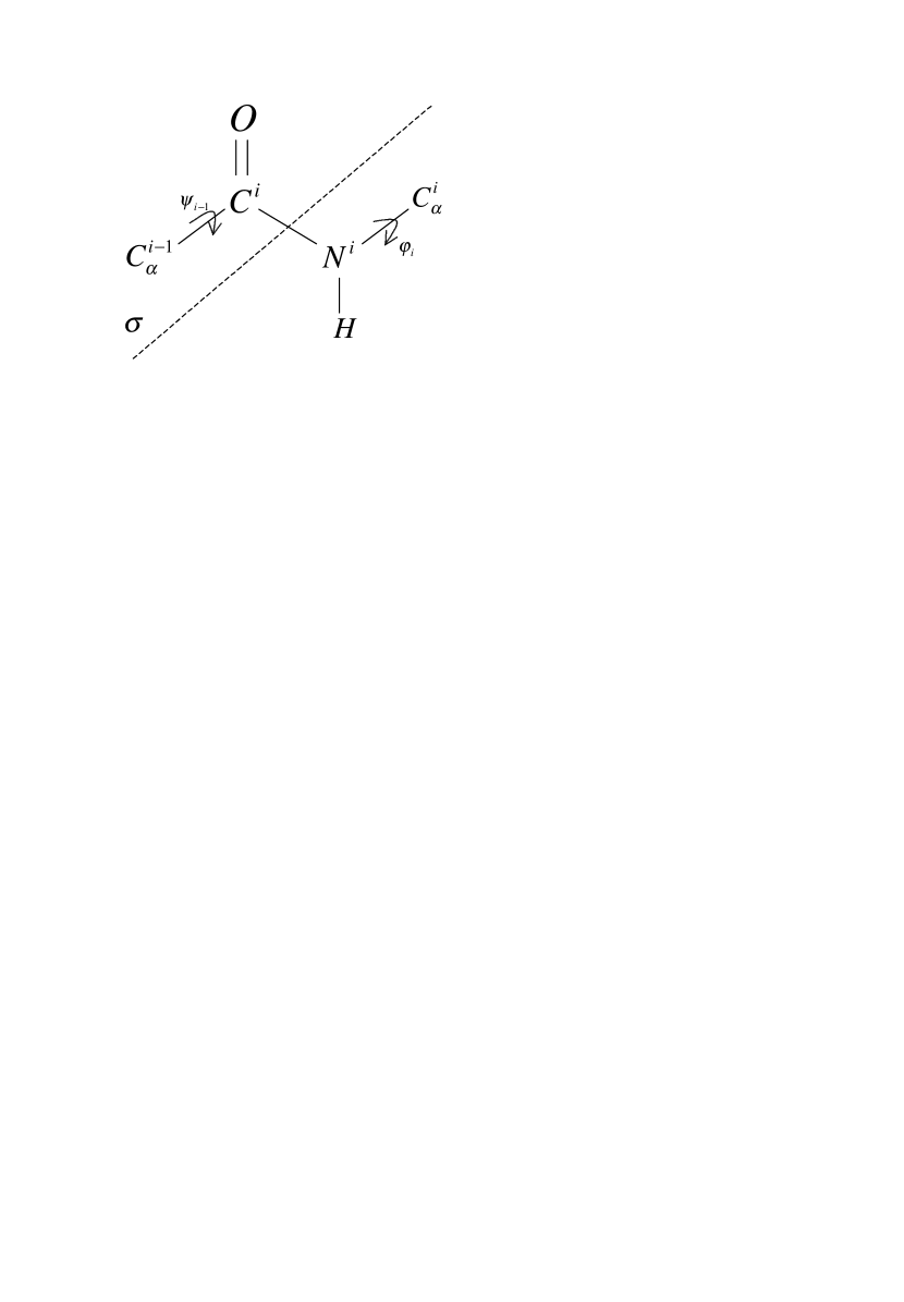
Figure 1: Schematic picture of the peptide group.

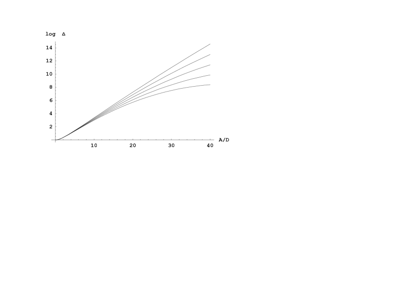
Figure 8: The dependence of the escape rate enhancement on the driving amplitude to noise intensity ratio for the case of quartic (bistable) potential $U(q)=-q^{2}/2+q^{4}/4$. The values of the noise intensity $D$ from the down line to the upper one respectively are: $5\cdot 10^{-3}$; $4\cdot 10^{-3}$; $3\cdot 10^{-3}$; $2\cdot 10^{-3}$; $1\cdot 10^{-3}$.

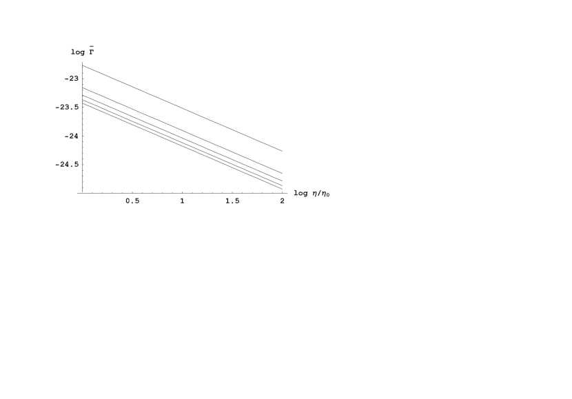
Figure 9: Dependence of the reaction rate constant $\bar{\Gamma}$ on solvent viscosity $\eta$ in the $log\ \bar{\Gamma}$ vs. $log\ \left(\eta/\eta_{0}\right)$ coordinates given by formula (52) for the case of quartic (bistable) potential. The values of $\left(A/D\right)_{0}$ from the down line to the upper one respectively are: 1, 6, 11, 16, 21.

References

- [1] B. Gavish, M.M. Werber, Viscosity-Dependent Structural Fluctuations in Enzyme Catalysis, Biochemistry 18 (1979) 1269-1275.
- [2] D. Beece, L. Eisenstein, H. Frauenfelder, D. Good, M. C. Marden, L. Reinisch, A. H. Reynolds, L. B. Sorensen and K. T. Yue, Solvent Viscosity and Protein Dynamics, Biochemistry, 19 (1980) 5147- 5157.
- [3] H. Frauenfelder, F. Parak, R.D. Young, Conformational substates in proteins, Ann.Rev.Biophys.Chem. 17 (1988) 451-479.
- [4] A.P. Demchenco, C.I. Rusyn, E.A. Saburova, Kinetics of the lactate dehydrogenase reaction in high-viscosity media, Biochem. et Biophys. Acta 998 (1989) 196-203.
- [5] H. Frauenfelder, N. A. Alberding, A. Ansari et al., Proteins and pressure, J. Phys. Chem. 94 (1990) 1024-1037.
- [6] K. Ng, A. Rosenberg, Possible coupling of chemical to structural dynamics in subtilisin BPN’ catalyzed hydrolysis, Biophys Chem. 39 (1991) 57-68.
- [7] K. Ng, A. Rosenberg, The coupling of catalytically relevant conformational fluctuations in subtilisin BPN’ to solution viscosity revealed by hydrogen isotope exchange and inhibitor binding, Biophys Chem. 41 (1991) 289-99.
- [8] S. Yedgar, C. Tetreau, B. Gavish and D. Lavalette, Viscosity dependence of escape from respiratory proteins as a function of cosolvent molecular weight, Biophys. J. 68 (1995) 665-670.
- [9] W. Doster, Th. Kleinert, F. Post, M. Settles, Effect of solvent on protein internal dynamics, in: Protein-solvent interactions, Ed. R. B. Gregory, Dekker, N. Y., 1994.
- [10] Th. Kleinert, W. Doster, H. Leyser, W. Petry, V. Schwarz, M. Settles, Solvent composition and viscosity effects on the kinetics of CO binding to horse myoglobin, Biochemistry 37 (1998) 717-733.
- [11] H. Frauenfelder, P. G. Wolynes, R. H. Austin, Biological Physics, Rev. Mod. Phys. 71 (1999) 419-430.
- [12] S. A. Pabit, H. Roder, S. J. Hagen, Internal friction controls the speed of protein folding from a compact configuration, Biochemistry 43 (2004) 12532-12538.
- [13] H. Frauenfelder, P. W. Fenimore, G. Chen, B. H. McMahon, Protein folding is slaved to solvent motions, Proc. Natl. Acad. Sci. USA, 103 (2006) 15469-15472.
- [14] C.R. Welsh, ed., The fluctuating enzyme, Wiley, N.Y., 1986.
- [15] W. Doster, Viscosity scaling and protein dynamics, Biophys. Chem. 17 (1983) 97-103.
- [16] B. Gavish, Position-dependent viscosity effects on rate coefficient, Phys.Rev.Lett. 44 (1980) 1160-1163.
- [17] G. Barshtein, A. Almagor, S. Yedgar, B. Gavish, Inhomogeneity of viscous aqueous solutions, Phys. Rev. E52 (1995) 555-557.
- [18] R.F. Grote and J.T. Hynes, The stable states picture of chemical reactions. II. Rate constants for condensed and gas phase reaction models, J.Chem.Phys. 73 (1980) 2715-2732.
- [19] R. Zwanzig, Dynamical disorder: passage through a fluctuating bottleneck, J. Chem. Phys. 97 (1992) 3587-3589.
- [20] P. Hänggi, P. Talkner, M. Borkovec, Fifty years after Kramers’ equation: reaction rate theory, Rev.Mod.Phys. 62 (1990) 251-341.
- [21] B. Gavish, The role of geometry and elastic strains in dynamic states of proteins, Biophys. Struc. Mech. 4 (1978) 37-52.
- [22] B. Gavish, Molecular dynamics and the transient strain model of enzyme catalysis, in: C.R. Welsh, ed., The fluctuating enzyme, Wiley, N.Y., 1986.
- [23] B. Gavish, S. Yedgar, Solvent viscosity effects on protein dynamics: updating the concepts, in: Protein-solvent interactions, Ed. R. B. Gregory, Dekker, N. Y., 1994.
- [24] D. Antoniou, J. Basner, S. Nuñez and S.D. Schwartz, Computational and theoretical methods to explore the relation between enzyme dynamics and catalysis, Chem. Rev. 106 (2006) 3170-3187.
- [25] P.K. Agarwal, Role of protein dynamics in reaction rate enhancement by enzymes, J.Amer.Chem.Soc. 127 (2005) 15248-15256.
- [26] P.K. Agarwal, Enzymes: An integrated view of structure, dynamics and function, Microbial Cell Factories 5 (2006) 2-13.
- [27] H. Fröhlich, The extraordinary dielectric properties of biological materials and the action of enzymes, Proc.Natl.Acad.Sci. USA 72 (1975) 4211-4215.
- [28] H. Fröhlich, Coherence and the action of enzymes, in: C.R. Welsh, ed., The fluctuating enzyme, Wiley, N.Y., 1986.
- [29] A. Warshel, Energetics of enzyme catalysis, Proc. Natl. Acad. Sci. USA 75 (1978) 5250-5254.
- [30] A. Warshel, Dynamics of enzymatic reactions, Proc. Natl. Acad. Sci. USA 81 (1984) 444-448.
- [31] M. H. M. Olsson, W. W. Parson and A. Warshel, Dynamical contributions to enzyme catalysis: critical tests of a popular hypothesis, Chem. Rev. 106 (2006) 1737-1756.
- [32] M. H. M. Olsson, J. Mavri and A. Warshel, Transition state theory can be used in studies of enzyme catalysis: lessons from simulations of tunnelling and dynamical effects in lipoxygenase and other systems, Phil. Trans. R. Soc. B (2006) 361 (2006) 1417-1432.
- [33] A. Warshel, P. K. Sharma, M. Kato, Y. Xiang, H. Liu, and M. H. M. Olsson, Electrostatic basis for enzyme catalysis, Chem. Rev. 106 (2006) 3210-3235.
- [34] A.E. Sitnitsky, Fluctuations of electric field in enzyme active site as an efficient source of reaction activation, Chem. Phys. Lett., 240 (1995) 47-52.
- [35] A.E. Sitnitsky, Dynamical contribution into enzyme catalytic efficiency, Physica A371 (2006) 481-491; arXiv:cond-mat/0601165.
- [36] C.R. Cantor, P.R. Schimmel, Biophysical Chemistry, Freeman, San Francisco, 1980, part 1.
- [37] M. Go, N. Go, Fluctuations of an -helix, Biopolymers 15 (1976) 1119-1127.
- [38] J. A. McCammon, B. R. Gelin, M. Karplus, Dynamics of folded proteins, Nature 267 (1977) 585-590.
- [39] R. M. Levy, M. Karplus, Vibrational approach to the dynamics of an -helix, Biopolymers 18 (1979) 2465-2495.
- [40] W. F. van Gunsterent, M. Karplus, Protein dynamics in solution and in a crystalline environment: A molecular dynamics study, Biochemistry 21 (1982) 2259-2274.
- [41] M. Levitt, Molecular dynamics of native protein. II. Analysis and nature of motion, J. Mol. Biol. 168 (1983) 621-657.
- [42] M. J. Dellwo, A. J. Wand, Model dependent and model independent analysis of the global and internal dynamics of cyclosporin A, J. Am. Chem. Soc. 111 (1989) 4571-4578.
- [43] I. Chandrasekhar, G. M. Clore, A. Szabo, A. M. Gronenborn, B. R. Brooks, A 500 ps molecular dynamics simulation study of interleuin-1 in water: correlation with nuclear magnetic resonance spectroscopy and crystallography, J. Mol. Biol. 226 (1992) 239-250.
- [44] A. G. Palmer III, D. A. Case, Molecular dynamics analysis of NMR relaxation in a zinc-finger peptide, J. Am. Chem. Soc. 114 (1992) 9059-9067.
- [45] R. M. Brunne, K. D. Berndt, P. Guëntert, K. Wuëthrich, W. F. van Gunsteren, Structure and internal dynamics of the bovine pancreatic trypsin inhibitor in aqueous solution from longtime molecular dynamics simulations, Proteins 23 (1995) 49-62.
- [46] A. R. Fadel, D. Q. Jin, G. T. Montelione, R. M. Levy, Crankshaft motions of the polypeptide backbone in molecular dynamics simulations of human type- transforming growth factor, J. Biomol. NMR 6 (1995) 221-226.
- [47] M. Buck, M. Karplus, Internal and overall peptide group motion in proteins: Molecular dynamics simulations for lysozyme compared with results from X-ray and NMR spectroscopy, J. Am. Chem. Soc. 121 (1999) 9645-9658.
- [48] H. Déméné, I. P. Sugàr, Protein conformation and dynamics. Effects of crankshaft motions on 1H NMR cross-relaxation effects, J. Phys. Chem. A 103 (1999) 4664-4672.
- [49] T. S. Ulmer, B. E. Ramirez, F. Delaglio, A. Bax, Evaluation of backbone proton positions and dynamics in a small protein by liquid crystal NMR spectroscopy, J. Am. Chem. Soc. 125 (2003) 9179-9191.
- [50] G. M. Clore, C. D. Schwieters, Amplitudes of protein backbone dynamics and correlated motions in a small R/ protein: correspondence of dipolar coupling and heteronuclear relaxation measurements, Biochemistry 43 (2004) 10678-10691.
- [51] J. E. Fitzgerald, A. K. Jha, T. R. Sosnick, K. F. Freed, Polypeptide motions are dominated by peptide group oscillations resulting from dihedral angle correlations between nearest neighbors, Biochemistry 46 (2007) 669-682.
- [52] N. Flytzanis, A.V. Savin, Y. Zolotaryuk, Soliton dynamics in a thermalized molecular chain with transversal degree of freedom, Phys. Lett. A193 (1994) 148-153.
- [53] P. J. Rosskyt, M. Karplus, Solvation. A molecular dynamics study of a dipeptide in water, J. Am. Chem. Soc. 101 (1979) 1913-1937.
- [54] W. Doster, Brownian oscillator analysis of molecular motions in biomolecules, in: Neutron Scattering in Biology, Methods and Applications, Eds.: J. Fitter, T. Gutberlet and J. Katsaras, Springer, Berlin, 2006.
- [55] A.B. Rubin, Biophysics, v.1, Nauka, Moscow, 2004, Ch.14.
- [56] H. Metiu, D. W. Oxtoby, K.F. Freed, Hydrodynamic theory for vibrational relaxation in liquids, Phys. Rev. A 15 (1977) 361-371.
- [57] R.P. Klüner, A. Dölle, Friction coefficient and correlation times for anisotropic rotational diffusion of molecules in liquids obtained from hydrodynamic models and relaxation data, J. Phys. Chem. A101 (1997) 1657-1661.
- [58] C. V. Heer, Statistical mechanics, kinetic theory and stochastic processes, Academic Press, N.Y. 1972, Ch. X.
- [59] A.E. Sitnitsky, Spectral properties of conformational motion in proteins, J. Biol. Phys. 22 (1996) 187-196.
- [60] A.E. Sitnitsky, Modeling the correlation functions of conformational motion in proteins, J.Biomol.Struct.@Dyn. 17 (2000) 735-745.
- [61] A.E. Sitnitsky, Modeling the ”glass” transition in proteins, J.Biomol.Struct.@Dyn. 17 (2002) 595-605.
- [62] J. R. Chaudhuri, S. K. Banik, B. C. Bag, D. S. Ray, Analytical and numerical investigation of escape rate for a noise driven bath, Phys. Rev. E 63 (2001) 061111.
- [63] J. R. Chaudhuri, S. Chattopadhyay, S.K. Banik, Generalization of escape rate from a metastable state driven by external cross-correlated noise processes, Phys. Rev E 76 (2007) 021125.
- [64] P. Jung, Periodically driven stochastic systems, Phys.Reports 234 (1993) 175-295.
- [65] G.R. Fleming and P. Hänggi (eds.), Activated barrier crossing: applications in Physics, Chemistry and Biology, World Scientific, Singapore 1993.
- [66] P. Talkner and P. Hänggi (eds.), New trends in Kramers’ reaction rate theory, Kluwer, Dordrecht 1995.
- [67] J. Lehmann, P. Reimann, P. Hänggi, Surmounting oscillating barriers: Path-integral approach for weak noise, Phys.Rev. E62 (2000) 6282-6294.
- [68] V.N. Smelyanskiy, M.I. Dykman, B. Golding, Time oscillations of escape rates in periodically driven systems, Phys.Rev.Lett. 82 (1999) 3193-3197.
- [69] D. Ryvkine, M.I. Dykman, Noise-induced escape of periodically modulated systems: From weak to strong modulation, Phys Rev. E 72 (2005) 011110.
- [70] P. Carter, J. Wells, Dissecting the catalytic triad of a serine protease, Nature (London) 332 (1988) 564-568.
- [71] A.E. Sitnitsky, Discrete breathers in protein secondary structure, in: Soft Condensed Matter. New Research. Ed. K.I. Dillon, Ch.5, pp.157-172, Nova, 2007; arXiv:cond-mat/0306135.
- [72] B. Juanico, Y.-H. Sanejouand, F. Piazza, P. De Los Rios, Discrete Breathers in Nonlinear Network Models of Proteins, Phys. Rev. Lett. 99 (2007) 238104.
- [73] A.E. Sitnitsky, Low frequency limit for thermally activated escape with periodic driving, arXiv:cond-mat/0602232.