Anisotropic minimal conductivity of graphene bilayers

Abstract

Fermi line of bilayer graphene at zero energy is transformed into four separated points positioned trigonally at the corner of the hexagonal first Brillouin zone. We show that as a result of this trigonal splitting the minimal conductivity of an undoped bilayer graphene strip becomes anisotropic with respect to the orientation $\theta$ of the connected electrodes and finds a dependence on its length $L$ on the characteristic scale $\ell=\pi/\Delta k\simeq 50nm$ determined by the inverse of k-space distance of two Dirac points. The minimum conductivity increases from a universal isotropic value $\sigma^{min}_{\bot}=(8/\pi)e^{2}/h$ for a short strip $L\ll\ell$ to a higher anisotropic value for longer strips, which in the limit of $L\gg\ell$ varies from $(7/3)\sigma^{min}_{\bot}$ at $\theta=0$ to $3\sigma^{min}_{\bot}$ over an angle range $\Delta\theta\sim\ell/L$.

The recent realization of isolated graphene geim04 ; geim05 ; kim , a two dimensional hexagonal lattice of carbon atoms, and its bilayer geim06 has followed by intensive studies which explored many intriguing properties of these new carbon-based material castro-rmp . They are zero-gap semiconductors with their valance and conduction bands touching each other at the corners of the hexagonal first Brillouin zone, known as Dirac points. This specific band structure in connection with pseudo-spin aspect which characterizes the relative amplitude of electron wave function on two different sublattices of the hexagonal structure, have given the carriers a pseudo-relativistic chiral nature geim05 ; geim06 . The chirality is believed to be origin of most of peculiarities of quantum transport effects in single and bilayer graphene cheianov-prbr ; kats-natphys ; castro-rmp .

One of the most important observations in graphene systems is the existence of a nonzero minimal conductivity in the limit of vanishing carrier density (at Dirac point) geim05 . This effect which had been predicted theoretically long before the experimental synthesis of graphene fradkin , has been the subject of several recent theoretical investigations and in most studies a universal value $\sigma_{0}^{min}=(4/\pi)e^{2}/h$ for minimum conductivity of monolayer graphene was found ziegler ; gusynin ; peres ; katsnelson1 ; mirlin ; beenakker06 . Although the theoretical value is $\pi$ times smaller than the value measured in the early experiments, more recent experiments have confirmed the predicted universal value $\sigma_{0}^{min}$ for wide and short graphene strips lau ; morpurgo .

For bilayer graphene the minimum conductivity is also measured to be of order $e^{2}/h$ geim06 ; morozov . Despite the similarity of the chiral nature in single and bilayer graphene, the low energy spectrum in bilayer is drastically different from the linear dispersion of massless Dirac fermions in monolayer. The spectrum in bilayer, which has a parabolic form at high energies, acquires strong trigonal warping at low energies and undergoes the so called Lifshitz transition at which the Fermi line is broken into four separated pockets falko . In the limit of zero Fermi energy the pockets shrink into the points of which one is located at the Dirac point and three others positioned around it in a trigonal form (see Fig. 1(a)). The aim of the present letter is to study effect of this Dirac point trigonal splitting on the minimum conductivity of the bilayer, which will also allow to distinguish between the effects of masslessness and chirality. We employ the realistic model of a wide undoped bilayer strip of length $L$ as the scattering region connecting two highly doped regions as electrodes. Using a full Hamiltonian which takes into account all intra and interlayer hoppings between nearest neighbors atomic sites, we find that the effect of the trigonal splitting in the minimum conductivity depends on $L$ as compared to a characteristic length $\ell=\pi/\Delta k\simeq 50nm$ determined by the inverse of the k-space separation $\Delta k$ of two split Dirac points.

For a short strip of $L\ll\ell$ the effect of trigonal splitting is negligible and $\sigma^{min}_{\bot}=(8/\pi)e^{2}/h$, which is twice the minimum conductivity of a monolayer showing that in this limit the bilayer behaves as two independent single layer connected in parallel. For finite length strip the minimal conductivity increases above $\sigma^{min}_{\bot}$ and finds a dependence on the angle $\theta$ between the orientation of the electrodes and the hexagonal lattice symmetry axis. We find that for a long strip $L\gg\ell$ the anisotropic minimum conductivity $\sigma^{min}(\theta)$ increases from $(7/3)\sigma^{min}_{\bot}$ at $\theta=0$ to $3\sigma^{min}_{\bot}$ over an angle range $\Delta\theta\sim\ell/L$. Our results reveals importance of trigonal splitting of the zero energy spectrum on the minimal conductivity of bilayer graphene.

To this end, there have been few theoretical investigations devoted to the minimal conductivity in bilayer graphene katsnelson2 ; cserti-prb ; beenakker07 ; cserti-prl ; ando ; castro07 . In Ref. beenakker07 a wide bilayer sheet with a constant perpendicular interlayer hopping is considered to connect two heavily doped electrode regions. This model, which ignores the trigonal splitting, results in a minimum conductivity $\sigma^{min}=\sigma^{min}_{\bot}$ beenakker07 ; cserti-prb , establishing on the fact that for high energy electrons injected from the metallic electrodes, the constant interlayer hopping does not cause any significant effect and the bilayer sheets behaves as two monolayer in parallel. On the other hand authors of Refs. ando and cserti-prl have taken into account the effect of strong trigonal warping within, respectively, Born approximation and Kubo formula. They have found an isotropic and constant minimal conductivity $(24/\pi)e^{2}/h$, which is three times larger than $\sigma^{min}_{\bot}$ obtained in Refs. beenakker07 ; cserti-prb . However we note that the models employed in Refs. cserti-prl ; ando do not include the effect of electrodes which are present in a realistic experimental setup for conductivity measurement. This could be in particular important in graphene contacts due to the chirality of the carriers and the resulting Klein tunneling phenomena cheianov-prbr ; kats-natphys . Our study, taking into account both of the trigonal splitting and the electrodes effect, reveals anisotropy of the minimal conductivity and its dependence on $L/\ell$ which also clarifies the origin of the disagreement between the two above predictions.

We consider a ballistic bilayer graphene sheet in $x-y$ plane consisting of an undoped strip of length $L$ and width $W$ and two heavily doped regions for $x<0$ and $x>L$ on top of which bias electrodes are deposited. The interfaces between electrode regions and bilayer strip are oriented parallel to $y$ axis making an angle $\theta$ with respect to the symmetry axis of the bilayer lattice as indicated in Fig. 1(a).

Bilayer graphene is made of two coupled single layer graphene with different sites $A1,B1$ in the bottom layer and $A2,B2$ in the top layer. The two layers are arranged according to Bernal stacking in which every $A1$ site of bottom layer lies directly below an $A2$ site in the top layer, as shown in Fig. 1(a). Within the tight binding model of graphite castro-rmp ; castro07 we consider all the nearest neighbors hoppings. The unit cell of the bilayer lattice structure contains 4 sites $A1$, $B1$, $A2$, and $B2$. The intra-layer hoppings between the sites $A1-B1$ and $A2-B2$ are parameterized by the single energy $t\approx 3eV$. There are two type of inter-layer hoppings: $A1-A2$ and $B1-B2$ which are characterized by the energies $t_{\bot}\approx 0.4eV$ and $t_{3}\approx 0.3eV$, respectively.

   

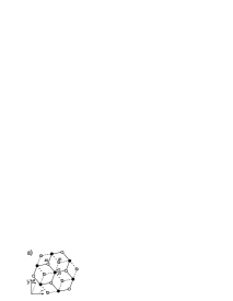
Figure 1: (a) The bilayer lattice structure projected onto the $x-y$ plane. Bonds between A1-B1 (A2-B2) in bottom (top) layer are indicated by dashed (solid) lines; $\theta$ is the angle between the hexagonal lattice symmetry axis and $y$-axis. (b) Constant-energy lines around the corner of the hexagonal first Brillouin zone for different energies (measured in units of Lifshitz transition energy $\varepsilon_{L}\approx 1meV$) near the neutrality point. Trigonally warped Fermi line is transformed into four separated points with one at the center and three positioned trigonally around it for $\varepsilon=0$.

The resulting tight binding Hamiltonian is written in k-space. The hexagonal first Brillouin zone of bilayer graphene contains 6 corners, among them two are inequivalent specifying the valleys $K$ and $K^{\prime}$. In the absence of inter-valley scattering castro-rmp , the valleys are degenerate and it is sufficient to consider only one valley. Low energy excitations with 2D wave vector ${\bf k}\equiv(k,q)$ around one of these valleys, say valley $K$, is governed by Hamiltonian of the form falko ,

$${\cal H}(\bf k)=\left(\matrix{0&\hbar vk_{-}&t_{\bot}&0\cr\hbar vk_{+}&0&0&\hbar v_{3}k_{-}\cr t_{\bot}&0&0&\hbar vk_{+}\cr 0&\hbar v_{3}k_{+}&\hbar vk_{-}&0}\right),$$ (1)

which operates in the space of 4-component spinors of the form $\Psi=e^{ikx+iqy}(\psi_{A1},\psi_{B1},\psi_{A2},\psi_{B2})$, where each component determines the wave function amplitude at the corresponding site of the bilayer unit cell. The characteristic velocities $v=3ta/(2\hbar)$,and $v_{3}=3t_{3}a/(2\hbar)$ ($a$ is the lattice constant) are associated with the hopping energies $t$ and $t_{3}$, respectively. We note that the complex wave vectors $k_{\pm}=e^{\mp i\theta}(k\pm iq)$ depend on the misorientation angle $\theta$.

The quasiparticle spectrum $\varepsilon(k,q)$ is obtained from the eigenvalue equation of Hamiltonian (1), which reads

$$(\varepsilon^{2}-|\hbar v{\bf k}|^{2})^{2}-\varepsilon^{2}(t_{\bot}^{2}+|\hbar v_{3}{\bf k}|^{2})+|\hbar v_{3}{\bf k}|^{2}t_{\bot}^{2}$$

$$=(\hbar v)^{2}t_{\bot}\hbar v_{3}(e^{3i\theta}(k-iq)^{3}+e^{-3i\theta}(k+iq)^{3}).$$ (2)

It is clear that the right hand side of this equation produces trigonal warping of constant-energy lines, with an strength given by the ratio $\delta=v_{3}/v$. Fig. 1(b) shows constant-energy lines for three energies $\varepsilon/\varepsilon_{L}=0,0.8,2$, where $\varepsilon_{L}=t_{\bot}\delta^{2}/4$ is the characteristic energy at which the Lifshitz transition takes place. While at $\varepsilon=2\varepsilon_{L}$ the energy line, despite its strong trigonal warping, is a continuous line, at $\varepsilon=0.8\varepsilon_{L}$ it breaks into four pockets whose enclosed area decreases with lowering energy and finally at $\varepsilon=0$ shrinks into the four points. The central point is located at $|{\bf k}|=0$ and other three leg points at a constant distance $|{\bf k}|=\Delta k=t_{\bot}v_{3}/(\hbar v^{2})$ from the center and in the directions determined by angles $\theta_{n}=\arctan(q_{n}/k_{n})=\theta+2(n-1)\pi/3$, $n=1,2,3$ (see Fig. 1(b)).

Dirac point splitting will have two main effects on the transport of carriers through the bilayer strip. First it introduces a length scale $\ell=\pi/\Delta k=(\pi\hbar v)/(t_{\bot}\delta)\approx 50nm$ as the effective range of the scattering potential which could mix the states at the four Dirac points. This length scale is an order of magnitude larger than interlayer coupling length $l_{\bot}=\hbar v/t_{\bot}$ introduced in Ref. beenakker07 . For realistic graphene samples of few 100 nm length, $L>\ell$ and the variations over this new length scale should be taken into account. The potential profile varies over the length $L$ of the strip. For $L\lesssim\ell$ the scattering potential is short enough to cause strong inter Dirac point scattering and consequently the scattering states at these points are mixed. On the other hand for $L\gg\ell$ the states of the Dirac points are well separated and do not mix. Secondly, it causes an anisotropy of the scattering states due to the orientation of the leg points. As we will explain in the following, these effects result in a length-dependent anisotropic minimal conductivity for the bilayer strip.

Within the scattering formalism we find the transmission amplitude of electrons through the bilayer strip. An electronic state is specified by the energy $\varepsilon$ and the transverse wave vector $q$, which are conserved in the scattering process. We find the eigenstates of Hamiltonian (1) in three regions of left ($x<0$) and right ($x>L$) electrodes and the bilayer strip ($0<x<L$). In general for a given $\varepsilon$ and $q$ there are 4 values of longitudinal momentum $k$ (solutions of Eq. (2)) with 4 corresponding eigenstates in each region.

Inside the strip at the neutrality point $\varepsilon=0$, the 4 solutions ($k_{i}$, $i=1,...,4$) of Eq. (2) have the form

$$k_{1,2}=k^{\ast}_{3,4}=iq+\frac{\pi}{2\ell}e^{-3i\theta}(1\pm\sqrt{1+i\frac{8q\ell}{\pi}e^{3i\theta}}).$$ (3)

The corresponding eigenstates are given by

$$\phi_{1,2} = e^{ik_{1,2}x+iqy}(0,-\frac{e^{-i\theta}}{l_{\bot}},k_{1,2}-iq,0),$$ (4)

$$\phi_{3,4} = e^{ik_{3,4}x+iqy}(k_{3,4}+iq,0,0,-\frac{e^{i\theta}}{l_{\bot}}).$$ (5)

In general for a given $q$ all 4 states inside the strip are evanescent having complex $k_{i}(i=1,...,4)$ with exceptions of the Dirac points with $q_{0}=0$ and $q_{n}=(\pi/\ell)\sin(\theta_{n})$ ($n=1,2,3$) at which two of $k_{i}$s are real representing propagating states in the strip.

Inside the highly doped electrode regions a very large potential $-U_{0}$ is applied. We assume that for all states contributing in transport $\hbar vq\ll U_{0}$ provided that $U_{0}$ be much larger than all other energy scales in Hamiltonian (1). By this assumption the longitudinal momenta of all states inside electrode regions have a constant magnitude $k_{0}=U_{0}/\hbar v\gg q$. Inside each electrode for certain $q$ there are two right-going eigenstates,

$$\phi^{R}_{\pm}=e^{ik_{0}x+iqy}(1,e^{-i\theta},\pm 1,\pm e^{i\theta}),$$ (6)

and two left-going eigenstates,

$$\phi^{L}_{\pm}=e^{-ik_{0}x+iqy}(1,-e^{-i\theta},\pm 1,\mp e^{i\theta}).$$ (7)

For two left-going incident states from the left electrode ($x<0$) the scattering states in three different regions have the form

$$\Psi_{\pm}=\left\{\begin{array}[]{ll}\raisebox{2.84526pt}{$\phi_{\pm}^{R}+r^{\pm}_{+}\phi_{+}^{L}+r^{\pm}_{-}\phi_{-}^{L}$}&\raisebox{2.84526pt}{$\hskip 8.53581ptx<0$,}\\ \sum_{i=1}^{4}c_{i}^{\pm}\phi_{i}&\hskip 14.22636pt0<x<L,\\ \raisebox{-2.84526pt}{$t_{+}^{\pm}\phi_{+}^{R}+t^{\pm}_{-}\phi_{-}^{R}$}&\raisebox{-2.84526pt}{$\hskip 8.53581ptx>L$.}\end{array}\right.$$ (8)

where the coefficients $c_{i}^{\pm}$ and reflection and transmission amplitudes $r^{\pm}_{\pm}$, $t^{\pm}_{\pm}$ have to be determined by imposing the continuity condition of the wave functions at the boundaries $x=0,L$.

We calculate the conductance at zero temperature from Landauer-Buttiker formula,

$$\frac{G}{G_{0}}=\frac{W}{2\pi}\int_{-\infty}^{\infty}T(q)dq,$$ (9)

where $T(q)=|t_{+}^{+}|^{2}+|t_{+}^{-}|^{2}+|t_{-}^{+}|^{2}+|t_{-}^{-}|^{2}$ is the sum of transmission probabilities of the two states $\Psi_{\pm}$, and $G_{0}=4e^{2}/h$ is 4 times of conductance quantum to take into account the valley and spin degeneracies. The conductivity of the bilayer strip is obtained by the relation $\sigma=(W/L)G$.

We have obtained $T(q)$ as a function of the length $L$ and the orientation angle $\theta$. For a short strip with $L\ll\ell$ the transmission probability takes the form

$$T(q)=\frac{1}{\cosh^{2}[(q-q_{c})L]}+\frac{1}{\cosh^{2}[(q+q_{c})L]},$$ (10)

which shows two maxima at the point $q=\pm q_{c}=\pm{\rm arcsinh}(L/2l_{\bot})/L$. Around these points $T(q)$ decays exponentially within a scale of order $\Delta q\sim 1/L$ which for a short strip is much larger than $\Delta k=\pi/\ell$. Thus $T(q)$ is almost constant within the scale $\Delta k$ which implies that the Dirac point splitting and the associated anisotropy of the spectrum are not revealed in the transmission of the carriers. This is the result of strong mixing of the states around the 4 Diract points via scattering through the bilayer strip. The resulting isotropic minimum conductivity $\sigma^{min}_{\bot}=2\sigma^{min}_{0}$ which is twice of the minimum conductivity for a single layer.

Figure 2: Minimal conductivity in units of $\sigma^{min}_{\bot}=(8/\pi)(e^{2}/h)$ of a wide strip of undoped bilayer graphene versus its length $L$ for different orientations $\theta$ of the hexagonal lattice symmetry axis with respect to the electrodes. $L$ is measured in units of $\ell=\pi/\Delta k$ with $\Delta k$ being the k-space distance of two trigonally split Dirac points. The isotropic minimal conductivity $\sigma^{min}_{\bot}$ at $L\ll\ell$ increases with $L/\ell$ to higher values and becomes anisotropic.

For a finite $L/\ell$ the minimum conductivity increases above $\sigma^{min}_{\bot}$. This is shown in Fig. 2 where we have plotted $\sigma^{min}$ as a function of $L/\ell$ for different orientations $\theta$. For $L/\ell\gtrsim 1$ the increased minimum conductivity finds a $\theta$-dependence as the result of trigonal splitting of the Dirac point. In this case the anisotropy of $\sigma^{min}$ is spread over the range $0<\theta<\pi/6$. We note that the increase in $\sigma^{min}$ is associated with an oscillatory variation due to quantum interference effects in bilayer strip. Increasing $L/\ell$ further to approach the limit of a long strip $L\gg\ell$ the range of anisotropy becomes narrower. In this limit and for the angles not too close to $\theta=0,\pi/6$ we obtain the following relation for the transmission probability

$$T(q)=\sum_{n=0,3}\frac{1}{\cosh^{2}[\alpha_{n}(\theta)(q-q_{n}(\theta))L]},$$ (11)

where the summation is taken over 4 transverse coordinates of the Dirac points, $q_{n}$, with $\alpha_{0}=1$ and $\alpha_{n}(\theta)=3/(5-4\cos[2\theta_{n}])$ for $n=1,2,3$. This result shows that the transmission probability consists of 4 resonant peaks at the points $q_{n}$, whose width is of order $\Delta q\sim 1/L<<\Delta k$. The effect of the Dirac point splitting is, thus, revealed in the transmission process. For $\theta$ approaching $0$ and $\pi/6$ the transverse coordinates of the two resonant peaks $q_{0}\rightarrow q_{1}$ and $q_{1}\rightarrow q_{2}$, respectively, and the corresponding peaks overlap. For these cases Eq. (11) is not applicable, since we have considered four Dirac points contribution independently in this equation. In the case of $\theta=0$ from Eqs. (8) and (9) we find that the contribution of the conductivity from the peaks at $q_{0}=q_{1}=0$ is of order $\delta^{2}e^{2}/h$ which is negligibly small. So there are only contributions from the points $q_{2},q_{3}$ which results in a minimum conductivity $\sigma^{min}_{\theta=0}=(7/3)\sigma^{min}_{\bot}$. In contrast to $\theta=0$ case, for $\theta=\pi/6$ the overlapped resonant peaks makes the same contributions as two independent peaks. This gives a minimum conductivity $\sigma^{min}=3\sigma^{min}_{\bot}$. We find that for a long strip this value of the minimum conductivity is valid for all orientations $0\lesssim\theta<\pi/6$ except of the angles $\theta\lesssim\ell/L$ where the two peaks $q_{0},q_{1}$ have a significant overlap. Thus the minimum conductivity is anisotropic over the range $\Delta\theta\sim\ell/L$ and an amplitude $\Delta\sigma^{min}=(2/3)\sigma^{min}_{\bot}$.

In conclusion, we have studied conductivity of a wide strip of undoped bilayer graphene which connects two highly doped electrode regions. We have shown that due to the trigonal splitting of Dirac point at zero Fermi energy, the minimal conductivity $\sigma^{min}$ of the strip finds a dependence on the lattice symmetry axis orientation $\theta$ with respect to the electrodes. The anisotropy of $\sigma^{min}$ depends on the length of strip $L$ as compared to the characteristic length scale $\ell=\pi/\Delta k\simeq 50nm$ determined by the inverse of the k-space separation of two Dirac points. For a short strip of $L\ll\ell$, $\sigma^{min}$ takes an isotropic universal value $\sigma^{min}_{\bot}=(8/\pi)e^{2}/h$. For longer strips the minimal conductivity increases above this value in an anisotropic way. We have found that in the limit of $L\gg\ell$ the anisotropic minimal conductivity grows from $(7/3)\sigma^{min}_{\bot}$ at $\theta=0$ to $3\sigma^{min}_{\bot}$ when orientation is changed by the angle $\Delta\theta\sim\ell/L$.

References

- (1) K. S. Novoselov et al., Science 306, 666 (2004).
- (2) K. S. Novoselov et al., Nature 438, 197 (2005).
- (3) Y. Zhang et al., Nature 438, 201 (2005).
- (4) K. S. Novoselov et al., Nature Physics 2, 177 (2006).
- (5) A. H. Castro Neto, F. Guinea, N. M. R. Peres, K. S. Novoselov, and A. K. Geim, arXiv:0709.1163 (2007).
- (6) V. V. Cheianov and V. I. Fal’ko, Phys. Rev. B 74, 041403(R)(2006).
- (7) M. I. Katsnelson, K. S. Novoselov, and A. K. Geim, Nature Physics 2, 620 (2006).
- (8) E. Fradkin, Phys. Rev. Rev. B 63, 3263 (1986); P. A. Lee, Phys. Rev. Lett. 71, 1887 (1993).
- (9) K. Ziegler, Phys. Rev. Lett. 97, 266802 (2006).
- (10) V. P. Gusynin and S. G. Sharapov, Phys. Rev. Lett. 95, 146801 (2005); Phys. Rev. B 73, 245411 (2006).
- (11) N. M. R. Peres, F. Guinea, and A. H. Castro Neto, Phys. Rev. B 73, 125411 (2006).
- (12) M. I. Katsnelson, Eur. Phys. J. B 51, 157 (2006).
- (13) P. M. Ostrovsky, I. V. Gornyi, and A. D. Mirlin, Phys. Rev. B 74, 235443 (2006).
- (14) J. Tworzydlo et al., Phys. Rev. Lett. 96, 246802 (2006).
- (15) F. Miao et al., Science 317, 1530 (2007).
- (16) R. Danneau, F. Wu, M. F. Craciun, S. Russo, M. Y. Tomi, J. Salmilehto, A. F. Morpurgo, and P. J. Hakonen, arXiv:0711.4306 (2007).
- (17) S. V. Morozov et al., Phys. Rev. Lett. 100, 016602 (2008).
- (18) E. McCann and V. I. Fal’ko, Phys. Rev. Lett. 96, 086805 (2006).
- (19) M. I. Katsnelson, Euro. Phys. J. B 52, 151 (2006).
- (20) J. Cserti, Phys. Rev. B 75, 033405 (2007).
- (21) I. Snyman and C. W. J. Beenakker, Phys. Rev. B 75, 045322 (2007).
- (22) M. Koshino and T. Ando, Phys. Rev. B 73, 245403 (2006).
- (23) J. Cserti, A. Csordás, and G. Dávid, Phys. Rev. Lett. 99, 066802 (2007).
- (24) J. Nilsson, A. H. Castro Neto, F. Guinea, and N. M. R. Peres, arXiv:0712.3259 (2007).