Induced scattering of short radio pulses

Abstract

Effect of the induced Compton and Raman scattering on short, bright radio pulses is investigated. It is shown that when a single pulse propagates through the scattering medium, the effective optical depth is determined by the duration of the pulse but not by the scale of the medium. The induced scattering could hinder propagation of the radio pulse only if close enough to the source a dense enough plasma is presented. The induced scattering within the relativistically moving source places lower limits on the Lorentz factor of the source. The results are applied to the recently discovered short extragalactic radio pulse.

1 Introduction

Induced scattering could significantly affect radiation from sources with high brightness temperatures. The induced Compton scattering may be relevant in pulsars (Wilson & Rees 1978; Lyubarskii & Petrova 1996, Petrova 2004a,b, 2007a,b), masers (Zeldovich, Levich & Sunyaev 1972; Montes 1977) and radio loud active galactic nuclei (Sunyaev 1971; Coppi, Blandford & Rees 1993; Sincell & Coppi 1996). The induced Raman scattering is considered as the most plausible mechanism of eclipses in binary pulsars (Eichler 1991; Gedalin & Eichler 1993; Thompson et al. 1994; Luo & Melrose 1995) and was also invoked to place constraints on the models of pulsars (Lyutikov 1998; Luo & Melrose 2006) and models of intraday variability in compact extragalactic sources (Levinson & Blandford 1995).

Macquart (2007) used the induced Compton and Raman scattering in order to place limits on the observability of the prompt radio emission predicted (Usov & Katz 2000; Sagiv & Waxman 2002; Moortgat & Kuijpers 2005) to emanate from gamma-ray bursts. Recent discovery of an enigmatic short extragalactic radio pulse (Lorimer et al 2007) demonstrates that very high brightness temperature transients do exist in nature. In this paper, we address the induced scattering of short bright radio pulses. First we study the induced Compton and Raman scattering in the plasma surrounding the source. The central point is that due to the non-linear character of the process, the effective optical depth is determined not by the scale of the scattered medium but by the width of the pulse provided that the pulse is short in the sense that duration of the pulse is less than the light travel time in the scattered medium. For this reason, short enough pulses could propagate through the interstellar medium, contrary to Macquart’s claim. The induced scattering could hinder propagation of a high brightness temperature pulse only close enough to the source if the density of the ambient plasma is large enough; here we find the corresponding observability conditions. We also address the induced scattering within the relativistically moving source and show that transparency of the source implies a lower limit on the Lorentz factor of the source. We apply the general results to the short extragalactic radio pulse discovered by Lorimer et al. (2007).

2 Induced Compton scattering

The kinetic equation for the induced Compton scattering in the non-relativistic plasma is written as (e.g. Wilson 1982)

$$\frac{\partial n(\nu,\mathbf{\Omega})}{\partial t}+c(\mathbf{\Omega\cdot\nabla})n(\nu,\mathbf{\Omega})=\frac{3\sigma_{T}}{8\pi}N\frac{h}{m_{e}c}n(\nu,\mathbf{\Omega})\int(\mathbf{e\cdot e}_{1})^{2}(1-\mathbf{\Omega\cdot\Omega}_{1})\frac{\partial\nu^{2}n(\nu,\mathbf{\Omega}_{1})}{\partial\nu}d\mathbf{\Omega}_{1};$$ (1)

where $n(\nu,\mathbf{\Omega})$ is the photon occupation number of a beam in the direction $\mathbf{\Omega}$, $N$ the electron number density, $\mathbf{e}$ the polarization vector. The induced scattering rate is proportional to the number of photons already available in the final state therefore the scattering initially occurs within the primary emission beam where the radiation density is high. However, when the primary beam is narrow, as is anyway the case at large distance from the source, the recoil factor $1-\mathbf{\Omega\cdot\Omega}_{1}$ makes the scattering within the beam inefficient; then the scattering outside the beam dominates because according to Eq.(1), even weak isotropic background radiation (created, e.g., by spontaneous scattering) grows exponentially so that the energy of the scattered radiation becomes eventually comparable with the energy density in the primary beam.

In this and the next sections, we study the induced scattering outside of the source therefore we can assume that the scattering angle is larger than the small angle subtended by the primary radiation. In this case, the occupation number of the scattered photons varies according to the equation

$$\frac{1}{n}\frac{dn}{dt}=\frac{3\sigma_{T}}{8\pi}\frac{cN}{m_{e}}(\mathbf{e\cdot e}_{1})^{2}(1-\cos\theta)\frac{\partial}{\partial\nu}\left(\frac{F}{\nu}\right);$$ (2)

where $F=c^{-2}h\int\nu^{3}nd\mathbf{\Omega}$ is the local radio flux density of the primary radiation, $\theta$ the scattering angle. Solution to this equation is written as

$$n=n_{0}\exp{\tau_{C}};$$ (3)

where $n_{0}$ is the background photon density, $\tau_{C}$ the effective optical depth determined by the integral along the scattered ray, $\mathbf{r}=\mathbf{r}_{0}+c\mathbf{\Omega}(t-t_{0})$, as

$$\tau_{C}=\int\frac{3\sigma_{T}}{8\pi}\frac{cN}{m_{e}}(\mathbf{e\cdot e}_{1})^{2}(1-\cos\theta)\frac{\partial}{\partial\nu}\left(\frac{F}{\nu}\right)dt.$$ (4)

The intensity of the scattered radiation increases exponentially provided the photon spectrum of the primary beam, $F/\nu$, has a positive slope. Therefore the induced scattering is the most efficient just below the spectral maximum. If the radiation with a decreasing spectrum is detected, one can find the observability condition substituting the frequency derivative in Eq.(4) by $F/\nu^{2}$ at the observed frequency because the stimulated scattering rate thus estimated is lower than that near the spectral maximum. As the brightness temperature of the primary beam many orders of magnitude exceeds the brightness temperature of the background radiation, the fraction of the scattered photons remains small until $\tau_{C}$ reaches a few dozens. As a simple criterion for the observability of the primary radiation (the condition that the induced scattering does not affect the primary radiation), one can use the condition $\tau_{C}<10$.

In order to check this condition, one can substitute the undisturbed primary flux into Eq.(4). Let a radio pulse of the duration $\Delta t$ propagate radially from the source; then the primary flux can be presented in the form

$$F=\left(\frac{D}{r}\right)^{2}F_{\rm obs}\Theta\left(\frac{ct-r}{c\Delta t}\right);$$ (5)

where $D$ is the distance to the source, $r$ the distance from the source to the scattering point, the function $\Theta(x)$ describes the shape of the pulse. Below we adopt the simplest rectangular form: $\Theta(x)=1$ at $0<x<1$ and $\Theta(x)=0$ otherwise. Note that we can ignore the transverse structure of the pulse because the most efficient is the backscattering so that the scattered ray interacts only with the radiation emitted in the same direction.

Note also that even though Eq.(5) assumes that the pulse structure is attributed to the intrinsic time variation of the source, the same structure arises if pulsed radiation is generated by a narrow beam sweeping across the observer. In this case, the radiation field has a shape $\Theta\left[(ct-r-r_{0}\varphi)/c\Delta t\right]$, which is reduced to Eq.(5) at $\varphi=\it const$. However, one should take into account that in this paper, we assume that the pulse is single in the sense that the distance between pulses is larger than the scale of the scattering medium. If this condition is not fulfilled, the scattered ray could pass through a few pulses and then the induced scattering occurs as in the steady radiation field with the intensity equal to the average intensity of the source. Therefore the results of this paper should be applied only to true single events like radio emission from gamma-ray bursts or giant pulses from pulsars, which are rare enough to be considered as isolated phenomena.

Let a seed ray be launched in the point $r_{0}$ at the time $t_{0}=cr_{0}$ just when the pulse reached this point. Due to induced scattering of the photons from the pulse, the intensity of the ray grows exponentially while the ray remains within the zone illuminated by the pulse. Below we assume that the pulse is narrow enough, $c\Delta t\ll r_{0}$. In order to find the amplification factor of the seed ray, one should find the effective optical depth (4), which could be presented as

$$\tau_{C}=\frac{3\sigma_{T}}{8\pi}\frac{cNF_{\rm obs}}{m_{e}\nu^{2}}\left(\frac{D}{r_{0}}\right)^{2}Z$$ (6)

where

$$Z=\int(1-\cos\theta)\left(\frac{r_{0}}{r}\right)^{2}\Theta\left(\frac{ct-r}{c\Delta t}\right)dt$$ (7)

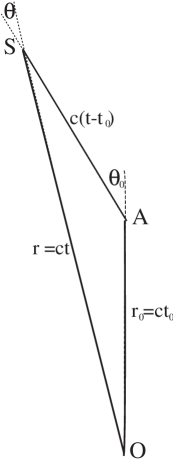
Figure 1: Geometry of the scattering. The primary pulse propagates radially from the point O. Just when it arrives at the point A (at the time $t_{0}$), a seed ray is launched at the angle $\theta_{0}$. At the time $t$, the seed ray arrives at the point S where it makes the angle $\theta$ with the radial direction.

is the integral along the ray. For the estimates, we take $\mathbf{e\cdot e}_{1}=1$. Let the ray be directed at the angle $\theta_{0}$ to the radial direction at the initial point. Then the scattering angle, $\theta$, and the distance from the source, $r$, at the time $t$ could be found from the laws of sines and cosines for the triangle in Fig. 1

$$\frac{c(t-t_{0})}{\sin(\theta_{0}-\theta)}=\frac{r_{0}}{\sin\theta};$$ (8)

$$r^{2}=r_{0}^{2}+c^{2}(t-t_{0})^{2}+2r_{0}c(t-t_{0})\cos\theta_{0}.$$ (9)

Eliminating $r$ and $t$, one can present the integral (7) as

$$Z=\frac{r_{0}}{c\sin\theta_{0}}\int_{\theta_{\rm min}}^{\theta_{0}}(1-\cos\theta)\theta d\theta=\frac{r_{0}}{c}\frac{\theta_{0}-\theta_{\rm min}-\sin\theta_{0}+\sin\theta_{\rm min}}{\sin\theta_{0}};$$ (10)

where $\theta_{\rm min}$ is determined from the condition that the function $\Theta$ vanishes, $r=c(t-\Delta t)$. This condition, together with Eqs.(8) and (9), yields the equation for $\theta_{\rm min}$

$$\frac{\tan\theta_{0}}{\tan\theta_{\rm min}}-1=\frac{\Delta t}{2t_{0}\cos\theta_{0}}\frac{2-\Delta t}{t_{0}(1-\cos\theta_{0})-\Delta t}.$$ (11)

Taking into account that $\theta_{0}-\theta_{\rm min}\ll 1$ at $\Delta t\ll t_{0}$, one gets

$$\theta_{\rm min}=\left\{\begin{array}[]{ll}\theta_{0}-\frac{c\Delta t\sin\theta_{0}}{r_{0}(1-\cos\theta_{0})};&\theta_{0}>\sqrt{\frac{2c\Delta t}{r_{0}}};\\ 0&\theta_{0}<\sqrt{\frac{2c\Delta t}{r_{0}}}.\end{array}\right.$$ (12)

If $\theta_{0}<\sqrt{2c\Delta t/r_{0}}$, the scattered ray remains within the illuminated area till infinity therefore $\theta_{\rm min}=0$ in this case. Finally one finds

$$Z=\left\{\begin{array}[]{ll}\Delta t\left(1-\frac{2c\Delta t}{r_{0}\theta_{0}^{2}}+\frac{4c^{2}\Delta t^{2}}{4r_{0}^{2}\theta_{0}^{4}}\right);&\theta_{0}>\sqrt{\frac{2c\Delta t}{r_{0}}};\\ \frac{r_{0}}{6c}\theta_{0}^{2}&\theta_{0}<\sqrt{\frac{2c\Delta t}{r_{0}}}.\end{array}\right.$$ (13)

One sees that the amplification factor is the same for all the scattered rays launched at not too small angles, $\theta_{0}\gg\sqrt{2c\Delta t/r_{0}}$. This is because decreasing of the scattering rate with decreasing angle (due to the recoil factor $1-\cos\theta$ in the scattering rate) is compensated by increasing of the time the scattered ray spends within the illuminated area. The rays launched at the angles $\theta_{0}\lesssim\sqrt{2c\Delta t/r_{0}}$ spend within the illuminated area the time $t-t_{0}\gtrsim r_{0}/c$; then the amplification factor decreases because of decreasing of the primary radiation density with the distance. Of course if the amplification factor is large, it is the backscattered radiation that takes the whole energy of the primary beam because the backward scattering is the fastest.

Substituting $Z=\Delta t$ into Eq.(6) one can now estimate the effective optical depth to the induced scattering; numerically one gets

$$\tau_{C}=0.24\frac{N_{6}\Delta t_{\rm s}F_{\rm obs,Jy}}{\nu_{\rm GHz}^{2}}\left(\frac{D_{8}}{r_{-3}}\right)^{2};$$ (14)

where $\Delta t_{\rm s}$, $F_{\rm obs,Jy}$ and $\nu_{\rm GHz}$ are measured in units shown in the index, $D=10^{8}D_{8}$ pc, $N=10^{6}N_{6}$ cm^-3, $r_{0}=10^{-3}r_{-3}$ pc. One sees that the induced scattering is negligible in the interstellar medium however it could become significant in dense enough environment close enough to the source. For example a massive star could be a progenitor of the gamma-ray burst; then the emission propagates through the relic stellar wind. In this case the plasma density falls off as

$$N_{6}=0.03\frac{\dot{M}_{-5}}{V_{3}r_{-3}^{2}};$$ (15)

where $\dot{M}=10^{-5}\dot{M}_{-5}$ $M_{\bigodot}\cdot$yr^-1 is the mass loss rate, $V=10^{3}V_{3}$ km$\cdot$s^-1 the wind velocity. The condition $\tau_{C}<10$ places the lower limit on the radius beyond which the radio pulse could propagate:

$$r_{-3}>0.16\left(\frac{D_{8}}{\nu_{\rm GHz}}\right)^{1/2}\left(\frac{\Delta t_{\rm s}F_{\rm obs,Jy}\dot{M}_{-5}}{V_{3}}\right)^{1/4}.$$ (16)

3 Induced Raman scattering

The high intensity radio beam could be scattered by emitting Langmuir waves. The energy and momentum conservation in this three-wave process require that

$$\nu_{1}=\nu+\nu_{p};\qquad\mathbf{k}_{1}=\mathbf{k}+\mathbf{q};$$ (17)

where $\nu_{p}=\sqrt{e^{2}N/(\pi m_{e})}$ is the plasma frequency, $\mathbf{q}$ the wave vector of the plasma wave. In the case $\nu\gg\nu_{p}$ one can neglect the frequency shift of the scattered wave; then one finds

$$\mathbf{q}_{\pm}=\pm\frac{\omega}{c}(\mathbf{\Omega}_{1}-\mathbf{\Omega}).$$ (18)

Here the sign $+$ is associated with a plasmon emitted by the photon $\mathbf{k}_{1}$ and the sign $-$ with a plasmon emitted by the photon $\mathbf{k}$. Because of Landau damping, only plasmons with large enough phase velocities could survive; this places a limit on the scattering angle (Thompson et al. 1994). Namely, choosing the allowable range of the plasmon wavevectors from the condition that the Landau damping time exceeds the period of the plasma wave, $q\lambda_{D}<0.27$, where $\lambda_{D}=\sqrt{k_{B}T/(4\pi e^{2}N)}$ is the Debye length, one finds from Eq. (18) that the backscattering is possible only if $\nu<\nu_{L}=90N_{6}^{1/2}T_{6}^{-1/2}$ MHz. In the case $\nu\gg\nu_{L}$, the maximum angle of scattering is

$$\theta_{\rm max}=2\nu_{L}/\nu.$$ (19)

The kinetic equations for the occupation numbers of photons and plasmons are written as (Thompson et al. 1994)

$$\frac{\partial n(\nu,\mathbf{\Omega})}{\partial t}+c(\mathbf{\Omega\cdot\nabla})n(\nu,\mathbf{\Omega})$$ (20)

$$=\frac{3\sigma_{T}}{8\pi}N\frac{h\nu}{m_{e}c}\frac{\nu}{\nu_{p}}\int(\mathbf{e\cdot e}_{1})^{2}(1-\mathbf{\Omega\cdot\Omega}_{1})[n_{q}+n_{-q}][n(\nu,\mathbf{\Omega}_{1})-n(\nu,\mathbf{\Omega})]d\mathbf{\Omega}_{1};$$

$$\frac{\partial n_{\pm q}}{\partial t}+v_{\rm g}((\mathbf{q}/q)\cdot\nabla)n_{\pm q}$$ (21)

$$=\frac{3\sigma_{T}}{8\pi}N\frac{h\nu}{m_{e}c}\frac{\nu}{\nu_{p}}\int(\mathbf{e\cdot e}_{1})^{2}\{n(\nu,\mathbf{\Omega}_{1})n(\nu,\mathbf{\Omega})\pm n_{\pm q}[n(\nu,\mathbf{\Omega}_{1})-n(\nu,\mathbf{\Omega})]\}d\mathbf{\Omega}_{1}-2\kappa n_{\pm q};$$

where $n_{q}$ is the plasmon occupation number, $\kappa$ the plasmon amplitude damping rate, $v_{\rm g}=3q\lambda_{D}\sqrt{k_{B}T/m_{e}}$ the plasmon group velocity. The last is small in the non-relativistic plasma therefore one can neglect the spatial transfer of plasmons.

As in the previous section, we assume that the primary radiation subtends the angle smaller than the scattering angle (19); then the scattering occurs outside the primary beam because the scattering within the beam is suppressed by the factor $1-\mathbf{\Omega\cdot\Omega}_{1}$. As in the previous section, we will find the observability condition demanding that the amplification factor of a weak background radiation due to the Raman scattering does not become exponentially large. One should stress that the Raman scattering does not necessary hinders propagation of the radiation even if the effective optical depth is large because the scattering angle (19) may be small. Then the radiation beam just widens and a special analysis is necessary in order to figure out how much parameters of the emerged radiation are affected. An example of such an analysis is given in sect. 5. Here we just find the effective optical depth to the Raman scattering.

Assuming that the primary pulse has the form (5) and that the intensity of the scattering radiation is small as compared with the primary radiation, one reduces the kinetic equations (20) and (21) to the form

$$\frac{\partial n}{\partial t}+c\cos\theta\frac{\partial n}{\partial r}=S\left(\frac{r_{0}}{r}\right)^{2}(1-\cos\theta)(n_{q}+n_{-q})\Theta\left(\frac{ct-r}{c\Delta t}\right);$$ (22)

$$\frac{\partial n_{\pm q}}{\partial t}=S\left[(n\pm n_{\pm q})\left(\frac{r_{0}}{r}\right)^{2}-\alpha n_{\pm q}\right]\Theta\left(\frac{ct-r}{c\Delta t}\right);$$ (23)

where

$$S=\frac{3\sigma_{T}}{8\pi}\frac{cNF_{0}}{m_{e}\nu\nu_{p}}\left(\frac{D}{r_{0}}\right)^{2}(\mathbf{e\cdot e}_{1})^{2};\qquad\alpha=\frac{F_{\kappa}}{F_{\rm obs}};\qquad F_{\kappa}=\frac{16\pi m_{e}\nu\nu_{p}}{3\sigma_{T}cN(\mathbf{e\cdot e}_{1})^{2}}\left(\frac{r_{0}}{D}\right)^{2}\kappa.$$ (24)

The plasmon decay rate due to electron-ion collisions is $\kappa=0.032N_{6}T_{6}^{-3/2}\,{\rm s}^{-1}$; then

$$F_{\kappa}=2.2\times 10^{-3}\frac{N_{6}^{1/2}\nu_{\rm GHz}}{T_{6}^{3/2}}\left(\frac{r_{-3}}{D_{8}}\right)^{2}\,\rm Jy.$$ (25)

We assume that before the pulse arrives, some weak background radiation preexists in the medium therefore the boundary conditions may be written as

$$n|_{r=ct}=n_{0};\qquad n_{q}|_{r=ct}=n_{q0}.$$ (26)

The factor $(r_{0}/r)^{2}$ in the right-hand side of Eqs. (22) and (23) arises due to decreasing of the primary radiation flux (5) with the distance. It was shown in the previous section that if the scattering angle is not too small, $\theta_{0}\gg\sqrt{2c\Delta t/r_{0}}$, the scattered ray remains within the illuminated area only during the time $t-t_{0}\ll r_{0}/c$; then the factor $(r_{0}/r)^{2}$ may be substituted by unity. Taking into account that the maximal scattering angle is given by Eq.(19), this condition is written as

$$\frac{N_{6}r_{-3}}{T_{6}\Delta t_{\rm s}\nu^{2}_{\rm GHz}}\gg 6\times 10^{-4}.$$ (27)

In this case, Eqs. (22) and (23) are easily solved. Namely, transforming the variables

$$v=Sct;\qquad u=S(ct-r);$$ (28)

one comes to the set of equations

$$\frac{\partial n}{\partial v}+(1-\cos\theta)\frac{\partial n}{\partial u}=(1-\cos\theta)(n_{q}+n_{-q})\Theta\left(\frac{u}{cS\Delta t}\right);$$ (29)

$$\frac{\partial n_{\pm q}}{\partial v}+\frac{\partial n_{\pm q}}{\partial u}=\left[n-(\alpha\mp 1)n_{\pm q}\right]\Theta\left(\frac{u}{cS\Delta t}\right);$$ (30)

with the boundary conditions at the point $u=0$. As both coefficients of the equations and the boundary conditions are independent of $v$, the solution is also independent of $v$ therefore one finally gets a simple set of ordinary differential equations at the segment $0<u<cS\Delta t$:

$$\frac{dn}{du}=n_{q}+n_{-q};\qquad\frac{dn_{\pm q}}{du}=n-(\alpha\mp 1)n_{\pm q}.$$ (31)

The boundary conditions are: $n(0)=n_{0}$, $n_{\pm q}(0)=n_{q0}$.

Partial solutions to these equations have a form $\exp(su)$ where $s$ obeys the characteristic equation

$$s^{3}+2\alpha s^{2}+(\alpha^{2}-3)s-2\alpha=0.$$ (32)

Simple solutions are found in the two limiting cases, namely when one can neglect the decay of plasmons, $\alpha=0$, and when the decay is strong, $\alpha\gg 1$ (these limits correspond to the conditions that the primary radiation flux is well above or well below the limiting flux (25), correspondingly). In the limit $\alpha=0$ the solution to Eqs.(31) is

$$n=\frac{1}{3}[n_{0}+2n_{0}\cosh\sqrt{3}u+2\sqrt{3}n_{q0}\sinh\sqrt{3}u];$$ (33)

$$n_{\pm q}=\frac{1}{3}[\mp n_{0}+(3n_{q0}\pm n_{0})\cosh\sqrt{3}u+\sqrt{3}(n_{0}\pm n_{q0})\sinh\sqrt{3}u].$$ (34)

In the limit $\alpha\gg 1$ the solution is

$$n=n_{0}\exp\left(\frac{2}{\alpha}u\right);$$ (35)

$$n_{\pm q}=\frac{n_{0}}{\alpha}\exp\left(\frac{2}{\alpha}u\right)+\left(n_{q0}-\frac{n_{0}}{\alpha}\right)\exp[(\pm 1-\alpha)u].$$ (36)

The intensity of the scattered radiation grows until $u=u_{\rm max}=S\Delta t$ so the effective optical depth to the Raman scattering may be estimated as $\tau_{R}=S\Delta t$ in the case $\alpha\ll 1$ and $\tau_{R}=S\Delta t/\alpha$ in the opposite limit. Numerically one gets

$$\tau_{R}=29\frac{N_{6}^{1/2}\Delta t_{\rm s}F_{\rm obs}}{\nu_{\rm GHz}}\left(\frac{D_{8}}{r_{-3}}\right)^{2}\left\{\begin{array}[]{ll}1;&F_{\rm obs}\gg F_{\kappa};\\ F_{\rm obs}/F_{\kappa};&F_{\rm obs}\ll F_{\kappa}.\end{array}\right.$$ (37)

As in the case of the induced Compton scattering, the condition for the Raman scattering to remain negligible may be written as $\tau_{R}<10$. One can see again that the scattering in the interstellar medium is negligible. Assuming that the emission is generated within the stellar wind of the progenitor star (see Eq.15), one obtains that the Raman scattering could be neglected if the radio pulse was emitted at the distance

$$r_{-3}>0.8D_{8}^{2/3}\left(\frac{\Delta t_{\rm s}F_{\rm obs,Jy}}{\nu_{\rm GHz}}\right)^{1/3}\left(\frac{\dot{M}_{-5}}{V_{3}}\right)^{1/6}\left\{\begin{array}[]{ll}1;&F_{\rm obs}\gg F_{\kappa};\\ (F_{\rm obs}/F_{\kappa})^{1/3};&F_{\rm obs}\ll F_{\kappa}.\end{array}\right.$$ (38)

from the source.

This result was obtained under the condition (27), i.e. if the scattering angle is not too small and the interaction of the scattered ray with the primary pulse occurs at the scale small enough that one can neglect decreasing of the primary radiation flux with radius. Therefore we neglected the factor $(r_{0}/r)^{2}$ in the right-hand side of Eqs.(22) and (23). In the opposite limit, the scattered ray remains within the illuminated zone for a long time however due to decreasing of the radiation flux, only the region $r-r_{0}\sim r_{0}$ contributes to the effective optical depth (cp. Eq.(13) and discussion after). As the solutions (33) and (35) are valid at $r-r_{0}<r_{0}$, one can find the amplification factor substituting into these solutions $u_{\rm max}$ corresponding to the radius $r=2r_{0}$. It follows from the scattering geometry (see Fig.1 and Eq.(9)) that $u_{\rm max}=Sr_{0}\theta_{0}^{2}/(4c)$. Substituting $\theta_{0}$ by the maximal scattering angle of Eq.(19), one gets finally the estimate for the effective optical depth at the condition opposite to that of Eq.(27)

$$\tau_{R}=2.4\times 10^{4}\frac{N_{6}^{3/2}F_{\rm obs,Jy}D_{8}^{2}}{T_{6}\nu^{3}_{\rm GHz}r_{-3}}\left\{\begin{array}[]{ll}1;&F_{\rm obs}\gg F_{\kappa};\\ F_{\rm obs}/F_{\kappa};&F_{\rm obs}\ll F_{\kappa}.\end{array}\right.$$ (39)

Note that within the range of applicability of this formula, it gives the optical depth smaller than Eq.(37).

4 Induced scattering within a relativistic source

If a high brightness temperature radio pulse is generated in a relativistic source, one can restrict parameters of the source considering stimulated emission within it. Let a radio pulse come from a relativistically hot plasma moving with the Lorentz factor $\Gamma$. In the comoving frame, the radiation could be considered as isotropic; then the kinetic equation for the induced Compton scattering could be written as (Melrose 1971)

$$\frac{1}{n(\nu^{\prime})}\frac{\partial n(\nu^{\prime})}{\partial t^{\prime}}=\frac{3}{16}\sigma_{T}\frac{h\nu^{\prime}}{m_{e}c}N^{\prime}\int d\gamma\frac{\partial}{\partial\gamma^{\prime}}\left(\frac{f(\gamma^{\prime})}{\gamma^{\prime 2}}\right)\int_{0}^{\infty}\frac{d\nu^{\prime}_{1}}{\nu^{\prime}_{1}}\left(1-\frac{\nu^{\prime}_{1}}{\nu^{\prime}}\right)g\left(\frac{\nu^{\prime}_{1}}{\nu^{\prime}}\right)n(\nu^{\prime}_{1});$$ (40)

where $f(\gamma^{\prime})$ is the electron distribution function normalized as $\int f(\gamma^{\prime})d\gamma^{\prime}=1$; the primed quantities are measured in the comoving frame. The kernel $g$ is approximated as (correcting a typo in Melrose’s paper)

$$g(x)=\left\{\begin{array}[]{ll}4x^{2};&(2\gamma^{\prime})^{-2}\leq x\leq 1;\\ 4x;&1\leq x\leq 4\gamma^{\prime 2};\\ 0;&{\rm otherwise}.\end{array}\right.$$ (41)

The right-hand side of Eq.(40) is the induced scattering rate; it should be compared with the rate of photon escape from the source, $c/l^{\prime}$, where $l^{\prime}$ is the characteristic size of the emitting region. If the emitting plasma moves, as is typically the case, radially from the origin, one should also take into account that the plasma density decreases in the proper frame with the rate $c\Gamma/r$. Then the condition that the induced scattering does not affect the emerged radiation is written as

$$\frac{1}{n(\nu^{\prime})}\frac{\partial n(\nu^{\prime})}{\partial t^{\prime}}<\max\left(\frac{c}{l^{\prime}},\frac{c\Gamma}{r}\right).$$ (42)

In order to estimate the stimulated scattering rate, let us assume that the particle distribution is Maxwellian

$$f(\gamma)=\frac{\gamma^{2}}{2\gamma_{T}^{3}}\exp\left(-\frac{\gamma}{\gamma_{T}}\right)$$ (43)

and that the radiation spectrum has a form

$$I(\nu^{\prime})=I_{0}\left\{\begin{array}[]{ll}(\nu^{\prime}/\nu^{\prime}_{0})^{a};&\nu^{\prime}<\nu^{\prime}_{0};\\ (\nu^{\prime}/\nu^{\prime}_{0})^{-b};&\nu^{\prime}>\nu^{\prime}_{0};\end{array}\right.$$ (44)

where $I(\nu^{\prime})=h\nu^{\prime 3}n(\nu^{\prime})/c^{2}$ is the radiation intensity, $a>2$, $b>0$. The frequency of the photon decreases in the course of stimulated scattering in the isotropic medium therefore the right-hand side of Eq.(40) is positive for $\nu^{\prime}<\nu^{\prime}_{0}$. Upon integrating one gets

$$\frac{1}{n(\nu^{\prime})}\frac{\partial n(\nu^{\prime})}{\partial t^{\prime}}=\frac{3}{8}\frac{\sigma_{T}N^{\prime}cI_{0}}{m_{e}\gamma_{T}^{3}\nu^{\prime}_{0}\nu^{\prime}}\Phi\left(\frac{\nu^{\prime}_{0}}{4\gamma_{T}^{2}\nu^{\prime}}\right);$$ (45)

$$\Phi(x)=\frac{a+b}{(a-1)(b+1)}e^{-\sqrt{x}}+\frac{x^{-(a-1)}}{a-1}\int_{0}^{\sqrt{x}}y^{2(a-1)}e^{-y}dy$$

$$-\frac{x^{b+1}}{b+1}\int_{\sqrt{x}}^{\infty}y^{-2(b+1)}e^{-y}dy=\left\{\begin{array}[]{ll}(\frac{a+b}{(a-1)(b+1)}&x\ll 1;\\ \frac{\Gamma(2a-1)}{a-1}x^{-(a-1)};&x\gg 1;\end{array}\right.$$ (46)

where $\Gamma(x)$ is the gamma-function. One sees that the scattering rate is maximal at $\nu^{\prime}\sim\nu^{\prime}_{0}/(2\gamma_{T})^{2}$, the exact value depending on $a$ and $b$. Substituting $\nu^{\prime}=\nu^{\prime}_{0}/(2\gamma_{T})^{2}$ and $\Phi=1$, one gets an estimate of the induced scattering rate:

$$\frac{1}{n}\frac{\partial n}{\partial t^{\prime}}=\frac{3}{2}\frac{\sigma_{T}N^{\prime}cI_{0}}{m_{e}\gamma_{T}\nu^{\prime 2}_{0}}.$$ (47)

In order to check the observability condition (42), one should substitute $\nu^{\prime}_{0}=\nu_{\rm obs}/\Gamma$ into the formula (47) for the induced scattering rate and express $I_{0}$ via the observed flux. If the source size is small so that the proper light travel time, $l^{\prime}/c$, is less than the proper expansion time, $r/(c\Gamma)$, the source radiates within the angle $1/\Gamma$ and the luminosity may be expressed via the observed flux as $L=(\pi/2)F_{\rm obs}\nu_{\rm obs}D^{2}\Gamma^{-4}$. On the other hand, the luminosity, which is the relativistic invariant, could be calculated in the proper frame as $L=8\pi^{2}l^{\prime 2}\nu^{\prime}_{0}I_{0}$ (assuming the source is spherical in the comoving frame). This yields

$$I_{0}=\frac{F_{\rm obs}D^{2}}{16\pi\Gamma^{3}l^{\prime 2}};\qquad l^{\prime}<\frac{r}{\Gamma}.$$ (48)

In the opposite case $l^{\prime}>r/\Gamma$, one can imagine a radially expanding plasma radiating forward so that the local radiation flux is $F\nu=4W^{\prime}c\Gamma^{2}$, where $W^{\prime}=4\pi I_{0}\nu^{\prime}_{0}/c$ is the radiation density in the comoving frame. Then one can write

$$I_{0}=\frac{F_{\rm obs}D^{2}}{16\pi\Gamma r^{2}};\qquad l^{\prime}>\frac{r}{\Gamma}.$$ (49)

Now the observability condition (42) is written as

$$\frac{3\sigma_{T}N^{\prime}F_{\rm obs}D^{2}}{32\pi\gamma_{T}m_{e}\nu_{\rm obs}^{2}}<\left\{\begin{array}[]{ll}\Gamma l^{\prime};&l^{\prime}<r/\Gamma;\\ r;&l^{\prime}>r/\Gamma.\end{array}\right.$$ (50)

For any specific radiation model, one can check the observability condition substituting parameters of the emitting plasma in Eq. (50).

For a rather general preliminary estimate, one can express the plasma density in the source via the fraction $\zeta$ of the plasma energy radiated in the pulse. Only a small fraction of the plasma energy could typically be radiated in the radio band so that one can expect $\zeta\ll 1$ however one can not exclude a priori a larger $\zeta$ (and even $\zeta>1$ for a Poynting dominated source). We will see that this uncertainty is compensated by a very weak dependence of the result on $\zeta$. If the source is small, $l^{\prime}<r/\Gamma$, the total radiated energy is estimated as $E_{\rm rad}=\pi D^{2}\nu_{\rm obs}F_{\rm obs}\Delta t_{\rm obs}/\Gamma^{2}$ whereas the total plasma energy in the source is $E_{\rm pl}=4\pi l^{\prime 3}N^{\prime}\gamma_{T}mc^{2}\Gamma$, where $m=m_{e}$ in the electron-positron plasma and $m=m_{p}$ in the electron-ion plasma. In the opposite limit, $l^{\prime}>r/\Gamma$, one should compare the plasma energy density, $\varepsilon_{\rm pl}=3mc^{3}N^{\prime}\gamma_{T}\Gamma^{2}$, with the radiation energy density, $\varepsilon_{\rm rad}=F_{\rm obs}\nu_{\rm obs}(D/r)^{2}$. Now one can write

$$N^{\prime}=\frac{F_{\rm obs}\nu_{\rm obs}D^{2}}{mc^{2}\gamma_{T}\zeta}\left\{\begin{array}[]{ll}\Delta t/(4l^{\prime 3}\Gamma^{3});&l^{\prime}<r/\Gamma;\\ 1/(3cr^{2}\Gamma^{2});&l^{\prime}>r/\Gamma.\end{array}\right.$$ (51)

Then the observability condition is written as

$$\frac{\sigma_{T}F_{\rm obs}^{2}D^{4}}{\zeta\gamma_{T}^{2}m_{e}mc^{2}\nu_{\rm obs}\Gamma^{2}}<\left\{\begin{array}[]{ll}128\pi l^{\prime 4}/(3c\Delta t);&l^{\prime}<r/\Gamma;\\ 32\pi r^{3};&l^{\prime}>r/\Gamma.\end{array}\right.$$ (52)

The light travel time arguments imply that $l^{\prime}<c\Delta t\Gamma$ if $l^{\prime}<r/\Gamma$ and $r<c\Delta t\Gamma^{2}$ in the opposite limit. Taking this into account, one finally finds that the observability condition implies a lower limit on the Lorentz factor of the source:

$$\Gamma>100\frac{F_{\rm obs,Jy}^{1/4}D^{1/2}_{8}}{\zeta^{1/8}\gamma_{T}^{1/4}(m/m_{e})^{1/8}(\Delta t_{\rm s})^{3/8}\nu_{\rm GHz}^{1/8}}.$$ (53)

Note that as the radiation within the source is nearly isotropic, the induced scattering is important only if it affects the spectrum of the radiation. In the case of the induced Compton scattering in the relativistically hot plasma, the photon frequency decreases $\sim 4\gamma_{T}^{2}$ times already in a single scattering therefore the observability condition for the induced Compton scattering is the condition that the source is just transparent with respect to this process. The frequency change in the Raman scattering is small therefore the corresponding observability condition is less restrictive.

5 Implications for the observed short extragalactic pulse

Let us apply the obtained general observability conditions to the enigmatic radio pulse recently found by Lorimer et al. (2007) in a pulsar survey at the frequency 1.4 GHz. The duration of the pulse was $\Delta t\leq 5$ ms, the energy in the pulse $F_{\rm obs}\Delta t=0.15\pm 0.05$ Jy$\cdot$s. The dispersion measure is an order of magnitude larger than the expected contribution from the Milky Way and moreover, no galaxy was found at the position of the source. This lead Lorimer et al. to conclude that the source of the pulse is on cosmological distance; they give a very rough estimate $D\sim 500$ Mpc. Origin of this pulse is obscure; Popov & Postnov (2007) argue, on the statistical grounds, that this event could be related to a hyperflare from an extragalactic soft gamma-ray repeater.

Substituting the parameters of the pulse into Eqs. (16), one concludes that if the pulse was generated within a stellar wind, the induced Compton scattering places the lower limit on the emission radius, $r>6\cdot 10^{14}(\dot{M}_{-5}/V_{3})^{1/4}$ cm. A stronger limit is imposed by the Raman scattering; Eq. (38) yields

$$r>5\cdot 10^{15}\left(\frac{\dot{M}_{-5}}{V_{3}}\right)^{1/6}\left(\frac{D}{500\rm Mpc}\right)^{2/3}\rm cm.$$ (54)

One should note that according to Eq.(19), the angle of the Raman scattering is small in this case, $\theta_{\rm max}=0.024(V_{3}/\dot{M}_{-5})^{1/6}T_{6}^{-1/2}$, so that the Raman scattering does not hinder propagation of the pulse. However, scattering even by this small angle implies the temporal smearing of the pulse above the observed limit unless the pulse was initially collimated within the angle $\vartheta<2.4\cdot 10^{-4}(\Delta t/5{\rm ms})^{1/2}$. In the last case, the initial radiation flux in the pulse should have been $(\vartheta/\theta_{\max})^{2}=10^{4}\Delta tT_{6}(\dot{M}_{-5}/V_{3})^{1/3}$ times larger than that estimated above under the no scattering assumption; then the induced scattering would imply even stronger constraints. Therefore in any case, the lower limit (54) for the emission radius is robust provided the pulse was generated within the relic stellar wind of the progenitor star.

The observed pulse was definitely generated within relativistic plasma. The induced Compton scattering within the source place a limit on the Lorentz factor of the emitting plasma. Substituting the observed parameters of the pulse into Eq. (53), one gets

$$\Gamma>3800\gamma_{T}^{-1/4}\left(\frac{\Delta t}{5\rm ms}\right)^{-5/8}\left(\frac{m_{e}}{\zeta m}\right)^{1/8}\left(\frac{D}{500\rm Mpc}\right)^{1/2}.$$ (55)

6 Conclusions

In this paper, we have analyzed the effect of induced Compton and Raman scattering on propagation of a short bright radio pulse. The work was motivated by predictions that such pulses could accompany gamma-ray bursts (Usov & Katz 2000; Sagiv & Waxman 2002; Moortgat & Kuijpers 2005) and by a recent discovery of a single extragalactic radio pulse (Lorimer et al. 2007). Macquart (2007) claimed that induced scattering in the interstellar medium strongly limits the observability of high brightness temperature transients. However he ignored two fundamental properties of the process. First of all, the induced scattering occurs only if the scattered ray remains within the zone illuminated by the scattering radiation. In the case of a single short pulse, the effective optical depth is determined by the duration of the pulse but not by the scale of the scattering medium. Therefore a short enough pulse could propagate freely through the interstellar medium. The second important property is that in the presence of a powerful radiation beam, even a weak background radiation grows exponentially via the induced scattering of the beam photons. If the primary beam is narrow, the scattering outside the beam dominates because the scattering within the beam is suppressed by the recoil factor $1-\mathbf{\Omega\cdot\Omega}_{1}$ in the scattering rate. Outside the source, the radiation subtends a small solid angle therefore the induced scattering in the surrounding medium occurs outside the beam. In this case, the effective optical depth depends not on the brightness temperature and the angle subtended by the primary radiation, which could not be found separately without model assumptions, but only on the radiation flux, which is a directly observable quantity. We demonstrated that the induced scattering in the surrounding medium could hinder the escape of a bright short pulse only if the source is embedded into a dense medium, like stellar wind. We estimated a limiting radius beyond which the pulse could propagate.

One should stress that these estimates assume a single pulse. If a sequence of pulses (e.g., pulsar emission) propagates in the medium with the characteristic scale exceeding the distance between the pulses, the induced scattering occurs as if the emission was steady with the average radiation flux. On the other hand, our results could be applied to giant pulses from pulsars, which are rare enough to be considered as isolated phenomena.

We have also analyzed induced scattering within the relativistically moving source. Transparency of the source is determined by the radiation intensity and by amount of plasma within the source. Introducing a fraction $\zeta$ of the plasma energy emitted in the pulse, we found a lower limit on the Lorentz factor of the source, which turned out to be very weakly dependent on $\zeta$.

References

- (1) Coppi, P., Blandford, R. D., & Rees, M. J. 1993, MNRAS, 262, 603
- (2) Gedalin, M., Eichler, D., 1993, ApJ, 406, 62
- (3) Eichler, D., 1991, ApJ, 370, L27
- (4) Levinson, A., Blandford, R., 1995, MNRAS, 274, 717
- (5) Lorimer, D. R.; Bailes, M.; McLaughlin, M. A.; Narkevic, D. J.; Crawford, F. 2007, Sci, 318, 777
- (6) Luo, Q., & Melrose, D. B. 1995, ApJ, 452, 346
- (7) Luo, Q., & Melrose, D. B. 2006, MNRAS, 371, 1395
- (8) Lyubarskii, Yu. E. & Petrova, S. A. 1996, AstL 22, 399
- (9) Lyutikov, M. 1998, MNRAS, 298, 1198
- (10) Macquart, J.-P., 2007, ApJ, 658, L1
- (11) Melrose, D. B. 1971, Ap&SS, 13, 56
- (12) Montes, C. 1977, ApJ, 216, 329
- (13) Moortgat, J., Kuijpers, J. 2005, gr-qc/0503074
- (14) Petrova, S. A. 2004a, A&A, 417, L29
- (15) Petrova, S. A. 2004b, A&A, 424, 227
- (16) Petrova, S. A. 2007a, arXiv0709.3173
- (17) Petrova, S. A. 2007b, arXiv0709.4578
- (18) Popov, S. B. & Postnov, K. A., 2007, arXiv:0710.2006
- (19) Sagiv, A., Waxman, E. 2002, ApJ, 574, 861
- (20) Sincell, M.W., & Coppi, P. S. 1996, ApJ, 460, 163
- (21) Sunyaev, R.A. 1971, Sov. Astron., 15, 190
- (22) Thompson, C., Blandford, R. D., Evans, C. R., Phinney, E. S., 1994, ApJ, 422, 304
- (23) Usov, V. V.; Katz, J. I. 2000, A&A, 364, 655
- (24) Wilson, D. B., 1982, MNRAS, 200, 881
- (25) Wilson, D. B. and Rees, M. J., 1978, MNRAS, 185, 297
- (26) Zel’dovich, Ya. B., Levich, E. V., & Sunyaev, R. A. 1972, Sov. Phys. JETP, 35, 733