Self-trapping of Bose-Einstein condensates expanding into shallow optical lattices

Abstract

We observe a sudden breakdown of the transport of a strongly repulsive Bose-Einstein condensate through a shallow optical lattice of finite width. We are able to attribute this behavior to the development of a self-trapped state by using accurate numerical methods and an analytical description in terms of nonlinear Bloch waves. The dependence of the breakdown on the lattice depth and the interaction strength is investigated. We show that it is possible to prohibit the self-trapping by applying a constant offset potential to the lattice region. Furthermore, we observe the disappearance of the self-trapped state after a finite time as a result of the revived expansion of the condensate through the lattice. This revived expansion is due to the finite width of the lattice.

I Introduction

The transport properties of Bose-Einstein condensates (BECs) through optical lattices have sparked interest in recent years after a series of experiments revealed dissipative dynamics and instabilities BhaMadMor97 ; BurCatFor01 ; MorMueCriCiaAri01 ; ScoMarBuj04 . Early experiments with BECs in optical lattices showed characteristic effects of such a periodic potential on atoms, namely, Bloch oscillations BenPeiRei96 and Josephson junctions AndKas98 ; CatBurFor01 . In later years the research focus shifted towards the study of nonlinear effects arising due to interaction of the atoms ChrMorMue02 . Theoretical work suggested that two mechanisms, energetic and dynamical instabilities, would lead to a dissipative dynamics WuNiu01 ; WuNiu03 . This dissipative behavior was also observed experimentally, and it was possible to separate dynamical and energetic instabilities BurCatFor01 ; FalSarLye04 ; SarFalLye05 . In a deep lattice it was found that increasing the nonlinearity leads to a self-trapped state within the lattice AnkAlbGat05 . Such a self-trapping effect was predicted theoretically in the limit of the tight-binding model TroSme01 . A generalized theoretical framework for the experiment in Ref. AnkAlbGat05 was derived in AleOstKiv06 , where it was pointed out that the experimental results can be explained in terms of a certain type of self-trapped state.

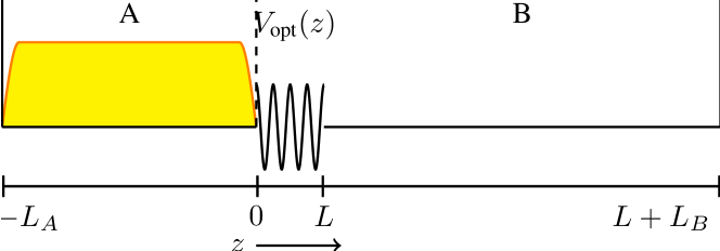
Figure 1: (Color online) Schematic setup of the system. The BEC is initially located in the flat-bottom box reservoir A. The shutter to its right (dashed vertical line) can be removed instantaneously so that the atoms expand into the optical lattice $V_{\text{opt}}(z)$ of size $L$. A wide potential-free region B serves as a second reservoir for the atoms. In our numerical calculations we used the dimensionless lengths $L_{A}=160\pi$, $L_{B}=326\pi$ and $L=10\pi$ (for an explanation of the units see text).

In this paper, we study the transport of a strongly interacting, one-dimensional (1D) BEC partially exposed to a shallow optical lattice of finite width. A typical experiment in this field is conducted by trapping atoms in a parabolic trap and then switching on a moving optical lattice. Alternatively, one can displace the parabolic trap in a stationary lattice, which leads to acceleration of the atoms through the lattice. We model these experiments by a simplified setup where two flat-bottom potentials are connected via the lattice as shown in Fig. 1. Instead of a moving lattice, we make use of the inherent expansion of the BEC. In contrast to experiments such as AnkAlbGat05 , in this present work we focus on the very shallow lattice regime, where the lattice depth is strictly less than the photon recoil energy. The theoretical study in AleOstKiv06 suggests that self-trapping is possible even at lower lattice depths but it does not take into account a short extent of the optical lattice. We extend previous works in this field by assuming an optical lattice of finite width connecting two reservoirs. Counterintuitively, even in the shallow lattice regime, we observe self-trapping for sufficiently high interaction strength. In contrast to spatially localized gap solitons ZobPoeMey99 , this type of localization extends over a few lattice sites without decay. The localization can be destroyed by applying a constant offset potential in the lattice region. The numerical analysis also shows that the finite width of the lattice results in the dissipation of the self-trapping after a finite time. We further compare the numerically obtained localized states with an analytical description. For our analytical results we incorporate nonlinear Bloch waves to approximate the self-trapped state. For the numerical treatment we simulate the 1D Gross-Pitaevskii equation (GPE), which is known to be a valid mean-field description at zero temperature DalGioPit99 . To study the dynamics of the system we use a second-order time-splitting spectral method (TSSP) to solve the GPE. This method is explicit, unconditionally stable and spectrally accurate in space. It is known to yield higher accuracy for the time evolution of the 1D GPE with less computational resources compared to, for example, Crank-Nicholson methods BaoJinMar02 ; BaoJakMar03 .

One of the underlying motivations of this field is a growing interest in the quantum transport of atoms for future microdevices. For such a device to become possible it will be necessary to identify basic building blocks—the equivalents of resistors, capacitors, transistors etc. in electronic devices— and to understand their interconnection BonSen04 . One approach is to use optical lattices to mimic the crystalline structure found in electronic devices SeaKraAnd07 . In classical electronic circuits such structures are found in wires and many fundamental components such as transistors or diodes. Recently, metallic behavior of ultracold atoms in three-dimensional optical lattices has been observed experimentally McKWhiPas08 . This finding further substantiates the analogy between electronic and atomic circuits. In an atomic circuit, atomic diodes RusMug04 ; HuWuDai07 and transistors MicDalJak04 would be connected by atom-transporting wires to build more complex devices. Such a wire can be constructed with a 1D optical lattice, which defines a band structure similar to the bands found in metals. In contrast to their electronic counterparts, the properties of atomic wires can be dynamically tuned in a precisely controllable way. By changing the angle, frequency or power of the lasers creating the lattice, the band structure of the medium can be adjusted to the required characteristics.

In Fig. 1 we sketch our full setup. The flat-bottom reservoirs A and B serve as a source and sink of a BEC, respectively. The BEC is initially confined to a potential-free box A. Such a flat-bottom potential has been implemented experimentally by Meyrath et al. MeySchHan05 . The short optical lattice connecting the reservoirs could be implemented by focusing two laser beams very tightly. However, we stress that our setup is to be understood rather as a generic theoretical model for a broader class of experimental setups, for example with shallow harmonic oscillator potentials as reservoirs. The difference in chemical potential on the left- and right-hand sides of this lattice leads to an expansion of the atoms into the lattice and eventually into reservoir B. In the atomic circuit picture, the setup can be seen as a battery, and the expansion of the atoms leads to a discharge current.

The paper is organized as follows. In Sec. II we will give a detailed overview of the model used and introduce the quantities of interest. Our numerical and analytical results of the transport properties of the BEC are explained in Sec. III. In the same section we also briefly discuss the creation of solitons, which are generated in our scheme. We conclude the paper with a summary in Sec. IV. An appendix provides details about the calculation of the nonlinear band structure of an interacting BEC in an optical lattice.

II The model

We consider a BEC at zero temperature in the elongated trap $V(x,y,z)=\tfrac{1}{2}m[\omega_{\perp}^{2}(x^{2}+y^{2})+V_{\text{ax}}(z)]$, where $m$ is the mass of an atom in the BEC. The transversal frequency $\omega_{\perp}$ is chosen to be $\hbar\omega_{\perp}\gg gn_{0}$, where $g$ the interaction strength of the atoms and $n_{0}$ the peak density of the BEC. In this paper we assume $g>0$, which corresponds to repulsive atomic interaction. The interaction strength can be expressed in terms of the s-wave scattering length $a_{s}$ as $g=4\pi\hbar^{2}a_{s}/m$. The above choice of the frequency $\omega_{\perp}$ results in the freezing of the atomic motion in the radial directions. Hence, we treat the BEC as an effectively one-dimensional condensate with a trapping potential $V_{\text{ax}}(z)$ along the axial direction Ols98 ; PetShlWal00 . In our model this potential has the form

$$V_{\text{ax}}(z)=\begin{cases}0&\quad\text{for }-L_{\text{A}}\leq z<0,\\ V_{\text{opt}}(z)&\quad\text{for }0\leq z\leq L,\\ 0&\quad\text{for }L<z\leq L+L_{\text{B}},\end{cases}$$ (1)

which is illustrated in Fig. 1. The condensate is initialized in the ground state of the box potential of size $L_{\text{A}}$, which is obtained by solving numerically the time-independent GPE using the normalized gradient flow method BaoDu04 ; BaoCheLim06 . After the initialization of the BEC in reservoir A, the shutter confining the BEC (dashed line in Fig. 1) is removed. The BEC then penetrates a short optical lattice $V_{\text{opt}}(z)=V_{0}+V_{1}\cos(2kz)$ of size $L\ll L_{\text{A}}$. We checked numerically that possible discontinuities in $V_{\text{ax}}$ at $z=0$ and $z=L$ do not affect the overall results. The periodicity $k$ is given by the geometry and wave number of the lasers producing the standing wave, and it determines the number of lattice sites $Lk/\pi$. The lattice height $V_{1}$ and the constant bias $V_{0}$ are assumed to be independently adjustable. The size of the sink reservoir B is $L_{\text{B}}\gg L$.

In order to obtain the dimensionless 1D GPE we introduce the following dimensionless quantities. Times are rescaled according to $\tilde{t}=t2E_{\text{R}}/\hbar$ and lengths according to $\tilde{z}=kz$, where $E_{\text{R}}=\hbar^{2}k^{2}/2m$ is the photon recoil energy. Inside the lattice region the potential Eq. (1) is given by $v_{\text{ax}}(z)=v_{\text{opt}}(z)=V_{\text{opt}}(\tilde{z})/E_{\text{R}}=v+s\cos(2\tilde{z})$ and zero otherwise. Hence, the dimensionless constant offset is $v=V_{0}/2E_{\text{R}}$ and the lattice depth $s=V_{1}/2E_{\text{R}}$. Furthermore, the wave function yields $\tilde{\psi}(\tilde{z},\tilde{t})=k^{-1/2}\psi(z,t)$. At $T=0$ the BEC can then be described by the dimensionless 1D GPE

$$\mathrm{i}\partial_{t}\psi=\left[-\frac{1}{2}\partial_{z}^{2}+v_{\text{ax}}(z)+\beta|\psi|^{2}\right]\psi,$$ (2)

where the tildes have been removed for clarity. The dimensionless interaction strength is $\beta=N_{\text{tot}}a_{s}k\hbar\omega_{\perp}/E_{\text{R}}$, which is expressed in terms of the number of atoms $N_{\text{tot}}$ and the s-wave scattering length $a_{s}$. The wave function $\psi=\psi(z,t)$ is normalized according to $\int|\psi(z,t)|^{2}\mathrm{d}z=1$ for all times $t$.

As an indicator of the dynamics of the system we define the dimensionless current

$$j(z,t)=\frac{1}{2\mathrm{i}}\left[\psi^{*}(z,t)\partial_{z}\psi(z,t)-\psi(z,t)\partial_{z}\psi^{*}(z,t)\right].$$ (3)

As will become apparent in the numerical analysis, it is advantageous to also define a more qualitative quantity, namely, the stationary current within the lattice. We compute the stationary current by taking the time derivative of the particle number in reservoir B, $N_{\text{B}}$, at times where the particle number $N$ within the lattice is nearly constant. Given a time $t_{0}$ with such a nearly constant particle number we define the stationary current as

$$j_{0}=\left.\frac{\mathrm{d}N_{\text{B}}}{\mathrm{d}t}\right|_{t_{0}}.$$ (4)

In general, the stationary current will depend on all parameters of the system such as the lattice depth $s$ or the interaction strength $\beta$.

III Breakdown of the atomic expansion

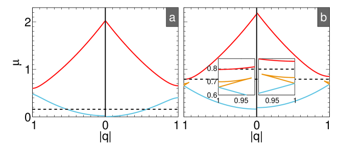
Figure 2: (Color online) Band structure for four sets of parameters $\mu$, $s$, and $n\beta$. The vertical line separates two sets with the same chemical potential (dashed line) but differing $s$ and $n\beta$. Note that each set is symmetric around $q=0$, hence we plot $|q|$. The offset $v$ is kept at zero. The other parameters are (a) $\mu=0.16$ ($\beta=79.58$) with $s=0.13$, $n\beta=0.05$ (left part) and $s=0.25$, $n\beta=0.04$ (right part), (b) $\mu=0.795$ ($\beta=397.89$) with $s=0.095$, $n\beta=0.329$ (left) and $s=0.127$, $n\beta=0.393$ (right). The left and right insets in (b) show a zoom of the loops near the left and right band edges, respectively.

Ignoring the finite width of the lattice, Eq. (2) reduces to to the well-known Mathieu equation in the limit of vanishing interaction ($\beta=0$). In this limit its energy eigenvalues develop the characteristic band structure of periodic potentials. The inclusion of the nonlinear term introduces a new energy scale $n\beta$ into the system ($n$ is the average particle density within the lattice), which changes the band structure. A net effect is an overall mean-field shift of the energies by $n\beta$. This effect is shown in Fig. 2(a) for typical parameters used in our simulations. For $n\beta>s$ the band structure additionally develops a loop at the band edge, which gradually decreases the width of the first band gap WuNiu00 ; DiaJenPet02 ; MacPetSmi03 . These loops can be observed in Fig. 2(b). The insets show a closeup of the band edges, where a loop has developed. Note that we only plot $|q|$ in a reduced zone scheme, which means that the loop closes symmetrically at $|q|>1$. The relative position of the chemical potential (dashed line in the figure) and the band gap will be important for the explanation of the localized state in the next subsection. For details about the calculation of the band structure we refer to the appendix.

III.1 Numerical results

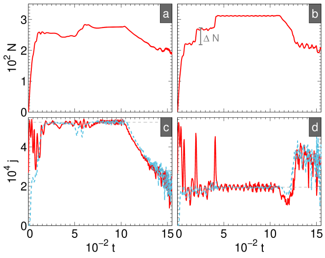
Figure 3: (Color online) Upper panel: time-dependent particle number within the lattice. Lower panel: time-dependent currents at the beginning of the lattice (red solid line) and the last lattice site (blue dashed). The gray dashed horizontal line indicates the stationary current obtained as described in the text. Lower panel: The parameters are $\beta=397.89$, $v=0$ for all plots and (a), (c) $s=0.095$ and (b), (d) $s=0.127$. The vertical bar in (b) indicates the analytical result for the particle number difference $\Delta N$ (see text).

In this section we will numerically investigate the transport of the BEC initially trapped in region A through the lattice. We will connect the various numerical findings and explain them in terms of self-trapped states with finite life time.

We have calculated the stationary current Eq. (4) numerically. Figures 3(a) and (b) show two typical time-dependent plots of the particle number within the lattice. We can recognize plateaux at different times in Figs. 3(a) and 3(b), which can be used to compute the stationary current. For example, in Fig. 3(b) such plateaux exist at the three time intervals $[0.008,0.019]$, $[0.021,0.04]$, and $[0.04,0.11]$. In the lower panel of Fig. 3 two typical results for the time-dependent current Eq. (3) are shown at different positions within the lattice. The dashed horizontal line indicates the stationary current corresponding to the same set of parameters. Note that its value coincides well with the actual current within the lattice for an extended amount of time. The current undergoes small oscillations around the value of the stationary current. The stationary current indicates the gross expansion speed of the BEC. We will analyze its dependence on the parameters $s$ and $\beta$ in the following.

Intuitively one expects the BEC in the setup of Fig. 1 to expand into the optical lattice where its transport properties are subjected to the modified band structure discussed above. We conducted numerical calculations in the regime of weak lattices ($s\ll 1$) and strong interaction ($\beta\gg 1$). If we plot the stationary current for different interaction strengths $\beta$ as a function of the optical lattice amplitude $s$, we notice a sharp drop in the curves for large $\beta$. In Fig. 4(a) this drop is clearly visible, whereas for the lower interactions in Fig. 4(b) it is absent in the shallow lattice regime. Note that the value of $j_{0}$ at $s=0$ increases with increasing $\beta$. This behavior is expected because the higher repulsive interaction leads to a higher potential difference between the reservoirs, which drives more atoms through the lattice region. An increase of the lattice amplitude does not influence the stationary current in Fig. 4(a) at first, instead it stays constant up to the drop. After the drop it decreases with increasing lattice depth.

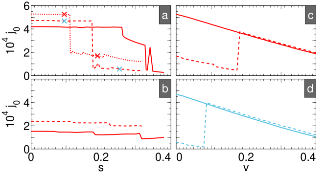
Figure 4: (Color online) Stationary current for (a), (b) varying $s$ at $v=0$ and (b), (c) varying constant offset $v$ at fixed $s$. Parameters for (a) are $\beta=251.46$ (solid line), $\beta=318.31$ (dashed), and $\beta=397.89$ (dotted), for (b) $\beta=31.83$ (solid) and $\beta=79.58$ (dashed). Plot (c) is at $\beta=397.31$ for fixed $s=0.095$ (solid line) and $s=0.19$ (dashed), (d) is at $\beta=318.31$ with $s=0.095$ (solid) and $s=0.253$ (dashed). The values for the lattice amplitude $s$ used in (c), (d) are marked in (a) on the curves with the respective interaction strengths.

We were able to relate the sudden drop in the stationary current to the development of an extended plateau in the time-dependent particle density within the lattice. In Fig. 3(b) we clearly recognize such a plateau for times around $4\times 10^{-2}$ to $11\times 10^{-2}$, as well as shorter plateaux at earlier times. For the parameters of this plot, $\beta=397.89$ and $s=0.127$, a drop in the stationary current has already occurred (cf. Fig. 4(a)). Also note that the drop can be observed in the time-dependent current in Fig. 3(d), which is lower than the current in Fig. 3(c). This means that after the drop, the BEC density within the lattice stays constant for an extended amount of time and there is only a small residual current flowing through the lattice. The BEC has effectively stopped its expansion despite its high repulsion and despite the lattice being very shallow. This fact can also be observed in a density plot of $|\psi(z,t)|^{2}$. Figure 5(a) shows the density of a BEC with a low interaction strength which does not show a drop in the stationary current. In contrast, the density for a higher $\beta$ which features a drop in the stationary current is plotted in Fig. 5(b). The value of $s$ in this plot was chosen larger than the value for the drop (cf. Fig. 4(a)). By comparing Fig. 5(b) with the particle number in Fig. 3(b) we also identify the steps in the plateau structure of the particle number as a tunneling of the BEC across lattice sites. Every time a lump of the BEC tunnels to the next lattice site, the average particle density increases by a fixed amount $\Delta N$ until it reaches a final lattice site where the expansion stops and a quasi-stationary state develops. For a fixed lattice height the final lattice site is determined by the value of $n\beta$ and $s$. This becomes clear by comparing the chemical potential in Fig. 2 (dashed horizontal line) with the position of the first band gap for a given set of parameters. For $\beta=79.58$, where the stationary current does not exhibit a drop, the chemical potential lies deep in the first band (cf. Fig. 2(a)). The atoms can populate the first band when being injected into the lattice region and move through the lattice. For very high $\beta$ however, the chemical potential initially lies above the first band gap (cf. Fig. 2(b)). As we increase $s$, the local chemical potential within the lattice $n\beta$ also increases slightly and shifts the band structure in such a way that the overall chemical potential $\mu$ falls into the first band gap. With its chemical potential lying inside the gap the wave function cannot expand anymore because there are no states available. This manifests itself in the development of the quasi-stationary state in Fig. 5(b). Increasing $s$ even further broadens the gap and the stationary current decreases steadily. We refer to this localized state as self-trapped state because its development strongly depends on the value of the nonlinearity $\beta$. We find the sudden onset of quasi-stationarity within the lattice only for high $\beta$, whereas for lower $\beta$ and large lattice amplitude the BEC does not penetrate the lattice. Alexander et al. AleOstKiv06 showed that such a self-trapped “gap wave” in a different setup remains stable. However, due to the shortness of the lattice in our setup, there is still a small current flowing through the lattice. This leakage eventually causes the localized state to disappear after a finite time. In Fig. 5(b) this breakdown can be observed for $t>1300$, when the BEC dissipates over the whole lattice. The phenomenon of such a finite life-time of the localized state has also been observed by Wang et al. in a different optical lattice setup WanFuLiu06 .

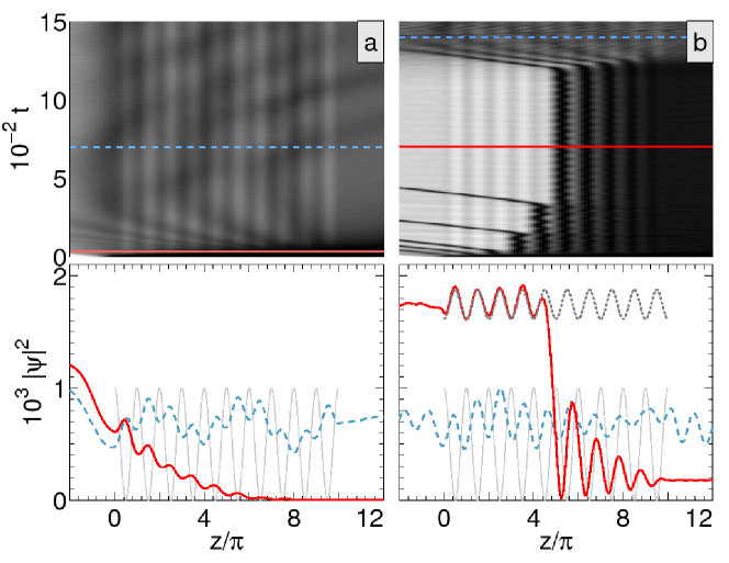
Figure 5: (Color online) Density plot of the BEC near the optical lattice. The lattice extends over $0\leq z\leq 10\pi$. In the upper panel light shades indicate high density, dark shades low density. For a typical rubidium BEC such as the one used in AnkAlbGat05 the time scale of these plots is around $32\,\mathrm{ms}$, which is experimentally accessible. The lower panel shows the profile of the BEC at the times indicated by the corresponding horizontal lines in the upper panel. The dotted line indicates the analytical result Eq. (10) for the corresponding nonlinear Bloch wave and the thin solid gray line indicates the position of the optical lattice. For both plots $s=0.127$, $v=0$ and (a) $\beta=79.58$, (b) $\beta=397.89$.

We further studied the case of a fixed $s$ with a varying offset potential $v$ confined to the lattice region. The two curves in each of Figs. 4(c) and 4(d) correspond to fixed values of $\beta$, respectively. The solid and dashed lines in each plot correspond to two different values of $s$. The lattice depths are chosen to lie before and after the drop in the stationary current. As expected, for a system whose chemical potential is located below the first band gap at $v=0$, the stationary current decreases with increasing offset potential (solid lines). In this case the offset shifts the whole band structure by a constant value. However, if the lattice depth is chosen such that the chemical potential lies in a band gap at $v=0$, we observe a sudden jump in the stationary current (dashed lines). This counterintuitive behavior, an increasing current for a higher potential barrier, can be explained by again noting that the constant offset shifts the band structure. Increasing the offset will eventually result in a band structure where the chemical potential does not lie in a gap anymore. Thus the jump occurs when the chemical potential rejoins a band.

III.2 Nonlinear Bloch waves

The GPE (2) with a periodic potential leads to the well-known Mathieu equation in the limit of vanishing interaction ($\beta=0$) if we assume a stationary state $\psi(z,t)=\exp(-\mathrm{i}\mu t)\psi_{q}(z)$. Here, $\mu$ is the chemical potential. The chemical potential of a BEC in the strongly interacting limit can be determined by utilizing the Thomas-Fermi approximation, which yields $\mu=\beta/L_{A}$. Our numerical calculations of the chemical potential of the initial 1D BEC are in good agreement with the Thomas-Fermi approximation for the parameters used in this paper. The solutions $\psi_{q}(z)$ are Bloch functions $\psi_{q}(z)=\exp(\mathrm{i}qz)\sum_{\ell=-\infty}^{\ell=\infty}c_{\ell}\exp(\mathrm{i}2\ell z)$. The parameter $q$ is the quasi-momentum of the condensate. To model the resulting wave function of the interacting case we similarly assume a Bloch function representation of the state. To simplify the analytical model we further truncate the Bloch waves according to MacPetSmi03

$$\psi_{q}(z)=\sqrt{n}\mathrm{e}^{\mathrm{i}qz}\left(c_{0}+c_{-1}\mathrm{e}^{-2\mathrm{i}z}+c_{1}\mathrm{e}^{2\mathrm{i}z}\right).$$ (5)

The density $n$ is defined as the averaged relative density of the BEC within the lattice

$$n=\frac{N}{L}.$$ (6)

The normalization of the full wave function $\psi(z)$ requires that $|c_{0}|^{2}+|c_{-1}|^{2}+|c_{1}|^{2}=1$. By using this method it is also possible to recover the band structure. For details of the calculation of the nonlinear band structure we refer to the appendix.

To understand the localization of the state after the drop consider Eq. (5) with parameters $\sqrt{n}c_{-1}=\sqrt{n}c_{1}=\mathrel{\mathop{\mathchar 58\relax}}d_{1}/2$ and $d_{0}\mathrel{\mathop{\mathchar 58\relax}}=\sqrt{n}c_{0}$. For the ground state with $q=0$ this results in the state

$$\psi(z)=d_{0}+d_{1}\cos(2z).$$ (7)

The normalization condition has to be rewritten as

$$|d_{0}|^{2}+\frac{1}{2}|d_{1}|^{2}=n.$$ (8)

The coefficients $d_{0}$ and $d_{1}$ can be determined by minimizing the energy functional under this constraint. This minimization procedure yields the two equations

$$2\beta d_{0}^{3}+d_{0}(3\beta d_{1}^{2}-2\mu)+sd_{1} =0,$$ (9a)

$$3\beta d_{1}^{3}+4d_{1}(2+3\beta d_{0}^{2}-\mu)+4sd_{0} =0,$$ (9b)

which can be solved analytically. Their real solution describes a nonlinear Bloch wave BroCarDec01 ; AleOstKiv06 . For the case of $q=0$ this wave function describes an oscillation with the period of the lattice around a finite value. To see this we assume a real solution of Eqs. (9) and calculate the density $|\psi(z)|^{2}$ from Eq. (7) to yield

$$|\psi(z)|^{2}=d_{0}^{2}+\frac{d_{1}^{2}}{2}+2d_{0}d_{1}\cos(2z)+\frac{d_{1}^{2}}{2}\sin(4z).$$ (10)

The constant offset in this equation is the particle density $n$ given in Eq. (8). The oscillation with the double period $4z$ can be neglected since for our parameter range $d_{1}^{2}/2\ll 2|d_{0}d_{1}|$. In the simulations we observe that for $s$ above the threshold for the drop in the stationary current, a quasi-stationary state develops. Figure 5(b) shows the development of such a localized nonlinear Bloch wave and its disappearance over time for high interaction strength. In the lower panel of Fig. 5(b) we show this behavior at two time slices. At early times the BEC tunnels across lattice sites as it expands into the lattice. At time $t\approx 700$ (solid line) we recognize the nonlinear Bloch wave in the lower panel of Fig. 5(b). The dotted line overlapping with the numerical curve is the analytical density Eq. (10) with the same parameters as the numerical result. We used the reduced chemical potential of the BEC still left in reservoir A and the lattice. We note that our analytical description of a nonlinear Bloch wave coincides well with the numerical result. At a later time $t\approx 1400$ (dashed line) the BEC is spread uniformly with a periodic modulation. In contrast, for values of $s$ and $\beta$ where the stationary current does not show a drop, the BEC spreads uniformly with time. The lattice region only slightly modulates the otherwise uniformly distributed atom density. In the lower panel of Fig. 5(a) we see that at $t\approx 30$ (solid line) the BEC has expanded into the optical lattice but the density is only slightly modulated with the period of the lattice. Similarly, at the later time $t\approx 700$ (dashed line) the now uniformly spread BEC is only slightly modulated by the periodic potential. A quasi-stationary nonlinear Bloch wave has not developed.

We further calculated the size of the steps between the plateaux in the particle number plot in Fig. 3(b). Integrating the particle density Eq. (8) over one lattice site yields

$$\Delta N=\pi\left(|d_{0}|^{2}+\frac{1}{2}|d_{1}|^{2}\right).$$ (11)

When the BEC advances one lattice site the particle number within the lattice should grow by $\Delta N$. The vertical bar in Fig. 3(b) indicates the analytically calculated difference Eq. (11) for the parameters used in the plot with a reduced chemical potential as discussed above. This result agrees with the difference of the numerically obtained particle number plateaux. Given the above agreements of analytical and numerical results we conclude that indeed the formation of a nonlinear Bloch wave causes the breakdown of the stationary current.

III.3 Dark solitons

The GPE supports soliton solutions for nonzero interaction $\beta$. These solutions are shape-preserving notches or peaks in the density which do not disperse over time. In the case of repulsive interaction without an optical lattice, solitons are typically of the dark type (notches in the density) BurBonDet99 ; CarBraBur01 but both dark and bright solitons can exist in BECs in optical lattices AlfKonSal02 ; StrGutPar02 . Our numerical results of the condensate density in Fig. 5(b) show the creation of moving dark solitons when the condensate jumps to a neighboring lattice site. In Fig. 5(b) we can see dark notches moving to the left, away from the lattice region. These excitations move slower than the local speed of sound ($c=\sqrt{\beta|\psi|^{2}}$) and do not change their shape considerably over the simulation time. We also observed other typical features of solitons such as the repulsion of two solitons approaching each other or the phase shift across a soliton. Furthermore, we notice that solitons emit sound waves traveling at the speed of sound. This happens when the center of mass of a soliton enters a region of different mean density, which causes a change in speed. A detailed analysis of soliton trajectories and their deformations in a nonuniform potential has been presented in ParProLea03 . It should be noted that the creation of moving solitons in our simulations shows similarities to the creation of solitonlike structures through self-interference of the BEC in hard-wall potentials RusKneSch01 . This self-interference could be caused by a small fraction of the BEC being reflected when the larger fraction tunnels through a peak of the optical lattice. Furthermore, it is worth noting that the exact dynamics and stability of the solitons also depends on the ratio $\mu/\omega_{\perp}~{}$MurShlErt02 . In our simulations we did not take into account the radial confinement, assuming that it is very tight and the overall BEC dynamics can be described by a quasi-1D model. We did hence not undertake a thorough analysis of the soliton dynamics in our system as their creation can be considered a side product of the development of the quasi-stationary state in the lattice, which was the main focus of this work.

IV Conclusion

We have investigated the effects of a finite width lattice on the transport properties of a strongly interacting BEC. To this end we numerically solved the corresponding 1D GPE and extracted relevant quantities such as the atomic current and density. We also compared the numerical with analytical results in terms of nonlinear Bloch waves.

We found that even for low lattice depths a quasi-stationary state develops after an initial expansion of the BEC into the lattice. This results in a sharp drop of the current in the lattice when the lattice depth and interaction reaches a critical value. However, due to the finite extent of the lattice the atoms can tunnel out of this state, which eventually leads to the breakdown of the stationarity. We could explain the development of a stationary state with partial nonlinear Bloch waves, which builds up over only a few lattice sites and blocks further atom flow. When we introduced a constant offset potential into the system, we found that increasing the offset can trigger the previously suppressed flow of the atoms again. Finally, we reported on the creation of moving dark solitons during the development of the nonlinear Bloch wave. Every time the BEC moves to a neighboring lattice site a soliton is emitted. Hence, the number of solitons present in the BEC indicates the number of occupied lattice sites.

In the context of atomic circuits the present work illuminates the role of wires in an atomic circuit. Our results suggest that by slightly increasing the lattice depth the superfluid current through the wire can be stopped easily. However, this effect is not based on a sudden Mott insulator transition since we always assumed the applicability of the GPE. In fact, it is based on a self-trapped macroscopic configuration, where the “charges” penetrate the wire to a certain depth but do not flow further.

*

Appendix A Nonlinear band structure

As discussed in Sec. III.2 we assume a wave function of the form Eq. (5). This trial function can be used to determine the energy spectrum of the system. In the noninteracting case this leads to the well-known linear band structure. The inclusion of the nonlinear term $\beta|\psi|^{2}$ with $\beta>0$ in the GPE modifies the band structure of the Mathieu eigenvalues. The overall mean-field shift of the band structure and the development of loops have been discussed in Sec. III. Their occurrence can be observed by assuming a trial function Eq. (5). We then rewrite the normalization condition of the coefficients $c_{\ell}$ in terms of two angles $\phi$ and $\theta$ according to

$$c_{0} =\cos\theta,$$ (12a)

$$c_{-1} =\sin\theta\sin\phi,$$ (12b)

$$c_{1} =\sin\theta\cos\phi.$$ (12c)

Stationary states can be found by plugging the ansatz Eq. (5) together with Eqs. (12) into the energy functional

$$\begin{split}\frac{\epsilon_{q}(\phi,\theta)}{n}&=\frac{1}{n\pi}\int_{0}^{\pi}\biggl{(}\frac{1}{2}|\nabla\psi_{q}(z)|^{2}+s\cos(2z)|\psi_{q}(z)|^{2}\\ &\phantom{=}+\frac{\beta}{2}|\psi_{q}(z)|^{4}\biggr{)}\mathrm{d}z.\end{split}$$ (13)

This integral is solved analytically and yields

$$\begin{split}\frac{\epsilon_{q}(\phi,\theta)}{n}&=\frac{q^{2}}{2}+2\sin^{2}\theta\,[1+q\cos(2\phi)]\\ &\hphantom{=}+\frac{s}{2}\sin(2\theta)\,(cos\phi+\sin\phi)\\ &\hphantom{=}+\frac{n\beta}{64}\Bigl{\{}43-\cos(4\phi)[3+\cos(4\phi)]\\ &\hphantom{=}-\cos(4\theta)[7+8\sin(2\phi)]\\ &\hphantom{=}+8\sin(2\phi)[1-\cos(2\theta)\sin(2\phi)]\Bigr{\}}.\end{split}$$ (14)

The first line represents the kinetic energy, the second line the lattice potential and the last three lines the interaction energy. By fixing different values of the quasi-momentum $q$ and minimizing Eq. (14) with respect to $\phi$ and $\theta$ we recover the band structure for given parameters $n\beta$ and $s$ (cf. Fig. 2).

References

- (1) C. F. Bharucha et al., Phys. Rev. A 55, R857 (1997).
- (2) S. Burger et al., Phys. Rev. Lett. 86, 4447 (2001), eprint cond-mat/0102076.
- (3) O. Morsch, J. H. Müller, M. Cristiani, D. Ciampini and E. Arimondo, Phys. Rev. Lett. 87, 140402 (2001), eprint cond-mat/0108457.
- (4) R. G. Scott et al., Phys. Rev. A 69, 033605 (2004).
- (5) M. Ben Dahan, E. Peik, J. Reichel, Y. Castin and C. Salomon, Phys. Rev. Lett. 76, 4508 (1996).
- (6) B. P. Anderson and M. A. Kasevich, Science 282, 1686 (1998).
- (7) F. S. Cataliotti et al., Science 293, 843 (2001), eprint cond-mat/0108117.
- (8) M. Cristiani, O. Morsch, J. H. Müller, D. Ciampini and E. Arimondo, Phys. Rev. A 65, 063612 (2002), eprint cond-mat/0202053.
- (9) B. Wu and Q. Niu, Phys. Rev. A 64, 061603(R) (2001), eprint cond-mat/0009455.
- (10) B. Wu and Q. Niu, New J. Phys. 5, 104 (2003), eprint cond-mat/0306411.
- (11) L. Fallani et al., Phys. Rev. Lett. 93, 140406 (2004), eprint cond-mat/0404045.
- (12) L. De Sarlo et al., Phys. Rev. A 72, 013603 (2005), eprint cond-mat/0412279.
- (13) T. Anker et al., Phys. Rev. Lett. 94, 020403 (2005), eprint cond-mat/0410176.
- (14) A. Trombettoni and A. Smerzi, Phys. Rev. Lett. 86, 2353 (2001).
- (15) T. J. Alexander, E. A. Ostrovskaya and Y. S. Kivshar, Phys. Rev. Lett. 96, 040401 (2006).
- (16) O. Zobay, S. Pötting, P. Meystre and E. M. Wright, Phys. Rev. A 59, 643 (1999), eprint cond-mat/9805228.
- (17) F. Dalfovo, S. Giorgini, L. P. Pitaevskii and S. Stringari, Rev. Mod. Phys. 71, 463 (1999), eprint cond-mat/9806038.
- (18) W. Bao, J. Shi and P. A. Markowich, J. Comput. Phys. 175, 487 (2002).
- (19) W. Bao, D. Jaksch and P. A. Markowich, J. Comput. Phys. 187, 318 (2003).
- (20) K. Bongs and K. Sengstock, Rep. Prog. Phys. 67, 907 (2004), eprint cond-mat/0403128.
- (21) B. T. Seaman, M. Krämer, D. Z. Anderson and M. J. Holland, Phys. Rev. A 75, 023615 (2007), eprint cond-mat/0606625.
- (22) D. McKay, M. White, M. Pasienski and B. DeMarco, Nature 453, 76 (2008), eprint 0708.3074.
- (23) A. Ruschhaupt and J. G. Muga, Phys. Rev. A 70, 061604(R) (2004), eprint quant-ph/0408133.
- (24) J. Hu, C. Wu and X. Dai, Phys. Rev. Lett. 99, 067004 (2007), eprint cond-mat/0703428.
- (25) A. Micheli, A. J. Daley, D. Jaksch and P. Zoller, Phys. Rev. Lett. 93, 140408 (2004), eprint quant-ph/0406020.
- (26) T. P. Meyrath, F. Schreck, J. L. Hanssen, C.-S. Chuu and M. G. Raizen, Phys. Rev. A 71, 041604(R) (2005), eprint cond-mat/0503590.
- (27) M. Olshanii, Phys. Rev. Lett. 81, 938 (1998), eprint cond-mat/9804130.
- (28) D. S. Petrov, G. V. Shlyapnikov and J. T. M. Walraven, Phys. Rev. Lett. 85, 3745 (2000), eprint cond-mat/0006339.
- (29) W. Bao and Q. Du, SIAM J. Sci. Comput. 25, 1674 (2004), eprint cond-mat/0303241.
- (30) W. Bao, I.-L. Chern and F. Y. Lim, J. Comput. Phys. 219, 836 (2006).
- (31) B. Wu and Q. Niu, Phys. Rev. A 61, 023402 (2000).
- (32) D. Diakonov, L. M. Jensen, C. J. Pethick and H. Smith, Phys. Rev. A 66, 013604 (2002), eprint cond-mat/0111303.
- (33) M. Machholm, C. J. Pethick and H. Smith, Phys. Rev. A 67, 053613 (2003), eprint cond-mat/0301012.
- (34) B. Wang, P. Fu, J. Liu and B. Wu, Phys. Rev. A 74, 063610 (2006), eprint cond-mat/0601249.
- (35) J. C. Bronski, L. D. Carr, B. Deconinck and J. N. Kutz, Phys. Rev. Lett. 86, 1402 (2001), eprint cond-mat/0007174.
- (36) S. Burger et al., Phys. Rev. Lett. 83, 5198 (1999).
- (37) L. D. Carr, J. Brand, S. Burger and A. Sanpera, Phys. Rev. A 63, 051601(R) (2001).
- (38) G. L. Alfimov, V. V. Konotop and M. Salerno, Europhys. Lett. 58, 7 (2002).
- (39) K. E. Strecker, G. B. Partridge, A. G. Truscott and R. G. Hulet, Nature 417, 150 (2002), eprint cond-mat/0204532.
- (40) N. G. Parker, N. P. Proukakis, M. Leadbeater and C. S. Adams, J. Phys. B 36, 2891 (2003), eprint cond-mat/0304148.
- (41) J. Ruostekoski, B. Kneer, W. P. Schleich and G. Rempe, Phys. Rev. A 63, 043613 (2001).
- (42) A. E. Muryshev, G. V. Shlyapnikov, W. Ertmer, K. Sengstock and M. Lewenstein, Phys. Rev. Lett. 89, 110401 (2002), eprint cond-mat/0111506.