Cross-correlation of long-range correlated series

Abstract

A method for estimating the cross-correlation $C_{xy}(\tau)$ of long-range correlated series $x(t)$ and $y(t)$, at varying lags $\tau$ and scales $n$, is proposed. For fractional Brownian motions with Hurst exponents $H_{1}$ and $H_{2}$, the asymptotic expression of $C_{xy}(\tau)$ depends only on the lag $\tau$ (wide-sense stationarity) and scales as a power of $n$ with exponent ${H_{1}+H_{2}}$ for $\tau\rightarrow 0$. The method is illustrated on (i) financial series, to show the leverage effect; (ii) genomic sequences, to estimate the correlations between structural parameters along the chromosomes.

Keywords: persistence (experiment), sequence analysis (experiment), scaling in socio-economic systems, stochastic processes

1 Introduction and overview

Interdependent behaviour and causality in coupled complex systems continue to attract considerable interest in fields as diverse as solid state science, biology, physiology, climatology [1, 2, 3, 4, 5, 6, 7, 8]. Coupling and synchronization effects have been observed for example in cardiorespiratory interactions, in neural signals, in glacial variability and in Milankovitch forcing [9, 10, 11]. In finance, the leverage effect quantifies the cause-effect relation between return $r(t)$ and volatility $\sigma_{T}(t+\tau)$ and eventually financial risk estimates [12, 13, 14, 15, 16, 17, 18, 19, 20, 21, 22, 23]. In DNA sequences, causal connections among structural and compositional properties such as intrinsic curvature, flexibility, stacking energy, nucleotide composition are sought to unravel the mechanisms underlying biological processes in cells [24, 25, 26].

Many issues still remain unsolved mostly due to problems with the accuracy and resolution of coupling estimates in long-range correlated signals. Such signals do not show the wide-sense-stationarity needed to yield statistically meaningful information when cross-correlations and cross-spectra are estimated. In [27, 28], a function $F_{xy}(n)$, based on the detrended fluctuation analysis - a measure of autocorrelation of a series at different scales $n$ - has been proposed to estimate the cross-correlation of two series $x(t)$ and $y(t)$. However, the function $F_{xy}(n)$ is independent of the lag $\tau$, since it is a straightforward generalization of the detrended fluctuation analysis, which is a positive-defined measure of autocorrelation for long-range correlated series. Therefore, $F_{xy}(n)$ holds only for $\tau=0$. Different from autocorrelation, the cross-correlation of two long-range correlated signals is a non-positive-defined function of $\tau$, since the coupling could be delayed and have any sign.

In this work, a method to estimate the cross-correlation function $C_{xy}(\tau)$ between two long-range correlated signals at different scales $n$ and lags $\tau$ is developed. The asymptotic expression of $C_{xy}(\tau)$ is worked out for fractional Brownian motions $B_{H}(t)$, $H$ being the Hurst exponent, whose interest follows from their widespread use for modeling long-range correlated processes in different areas [29]. Finally, the method is used to investigate the coupling between (i) returns and volatility of the DAX stock index and (ii) structural properties, such as deformability, stacking energy, position preference and propeller twist, of the Escherichia Coli chromosome.

The proposed method operates: (i) on the integrated rather than on the increment series, thus yielding the cross-correlation at varying windows $n$, as opposed to the standard cross-correlation; (ii) as a sliding product of two series, thus yielding the cross-correlation as a function of the lag $\tau$, as opposed to the method proposed in [27, 28]. The features (i) and (ii) imply higher accuracy, $n$-windowed resolution while capturing the cross-correlation at varying lags $\tau$.

2 Method

The cross-correlation $C_{xy}(t,\,\tau)$ of two nonstationary stochastic processes $x(t)$ and $y(t)$ is defined as:

$$C_{xy}(t,\tau)\equiv\Big{\langle}[x(t)-\eta_{x}(t)][y^{\ast}(t+\tau)-\eta_{y}^{\ast}(t+\tau)]\Big{\rangle}$$ (2.1)

where $\eta_{x}(t)$ and $\eta_{y}^{\ast}(t+\tau)$ indicate time-dependent means of $x(t)$ and $y^{\ast}(t+\tau)$, the symbol $\ast$ indicates the complex conjugate and the brackets $<>$ indicate the ensemble average over the joint domain of $x(t)$ and $y^{\ast}(t+\tau)$. This relationship holds for space dependent sequences, as for example the chromosomes, by replacing time with space coordinate. Eq. (2.1) yields sound information provided the two quantities in square parentheses are jointly stationary and thus $C_{xy}(t,\,\tau)\equiv C_{xy}(\tau)$ is a function only of the lag $\tau$.

In this work, we propose to estimate the cross-correlation of two nonstationary signals by choosing for $\eta_{x}(t)$ and $\eta_{y}^{\ast}(t+\tau)$ in Eq. (2.1), respectively the functions:

$$\widetilde{x}_{n}(t)=\frac{1}{n}\sum_{k=0}^{n}x(t-k)$$ (2.2)

and

$$\widetilde{y}_{n}^{*}(t+\tau)=\frac{1}{n}\sum_{k=0}^{n}y^{*}(t+\tau-k)$$ (2.3)

2.1 Wide-sense stationarity

The wide-sense stationarity of Eq. (2.1) can be demonstrated for fractional Brownian motions. By taking $x(t)=B_{H_{1}}(t)$, $y(t)=B_{H_{2}}(t)$, $\eta_{x}(t)$ and $\eta_{y}^{\ast}(t+\tau)$ calculated according to Eqs. (2.2,2.3), $C_{xy}(t,\,\tau)$ writes:

$$C_{xy}(t,\,\tau)=\Big{\langle}\big{[}B_{H_{1}}(t)-\widetilde{B}_{H_{1}}(t)\big{]}\big{[}B_{H_{2}}^{*}(t+\tau)-\widetilde{B}_{H_{2}}^{*}(t+\tau)\big{]}\Big{\rangle}\;\;\;.$$ (2.4)

When writing $x(t)=B_{H_{1}}(t)$ and $y(t)=B_{H_{2}}(t)$, we assume the same underlying generating noise $dB(t)$ to produce a sample of $x$ and $y$. Eq. (2.4) is calculated in the limit of large $n$ (calculation details are reported in the Appendix). One obtains:

$$C_{xy}(\hat{\tau}) =n^{H_{1}+H_{2}}D_{H_{1},\,H_{2}}\Big{[}-\hat{\tau}^{H_{1}+H_{2}}$$ (2.5)

$$+\frac{(1+\hat{\tau})^{1+H_{1}+H_{2}}+(1-\hat{\tau})^{1+H_{1}+H_{2}}}{1+H_{1}+H_{2}}$$

$$-\frac{(1-\hat{\tau})^{2+H_{1}+H_{2}}-2\hat{\tau}^{2+H_{1}+H_{2}}+(1+\hat{\tau})^{2+H_{1}+H_{2}}}{(1+H_{1}+H_{2})(2+H_{1}+H_{2})}\Big{]}\;\;\;,$$

where $\hat{\tau}=\tau/n$ is the scaled lag and $D_{H_{1},\,H_{2}}$ is defined in the Appendix. Eq. (2.5) is independent of $t$, since the terms in square parentheses depend only on $\hat{\tau}=\tau/n$, and thus Eq. (2.1) is made wide-sense stationary. It is worthy of note that, in Eq. (2.5), the coupling between $B_{H_{1}}(t)$ and $B_{H_{2}}(t)$ reduces to the sum of the exponents $H_{1}+H_{2}$. Eq. (2.5), for $\tau=0$, reduces to:

$$C_{xy}(0)\propto n^{H_{1}+H_{2}}\;\;\;,$$ (2.6)

indicating that the coupling between $B_{H_{1}}(t)$ and $B_{H_{2}}(t)$ scales as the product of $n^{H_{1}}$ and $n^{H_{2}}$. The property of the variance of fractional Brownian motion $B_{H}(t)$ to scale as $n^{2H}$ is recovered from the Eq. (2.6) for $x=y$ and $H_{1}=H_{2}=H$, i.e.:

$$C_{xx}(0)\propto n^{2H}\;\;\;.$$ (2.7)

Eq. (2.7) has been studied in [30, 31, 32, 33, 34].

3 Examples

3.1 Financial series

The leverage effect is a stylized fact of finance. The level of volatility is related to whether returns are negative or positive. Volatility rises when a stock’s price drops and falls when the stock goes up [12]. Furthermore, the impact of negative returns on volatility seems much stronger than the impact of positive returns (down market effect) [16, 17]. To illustrate these effects, we analyze the correlation between returns and volatility of the DAX stock index $P(t)$, sampled every minute from 2-Jan-1997 to 22-Mar-2004, shown in Fig. 1 (a). The returns and volatility are defined respectively as: $r(t)=\ln P(t+t^{\prime})-\ln P(t)$ and $\sigma_{T}(t)=\sqrt{{\sum_{t=1}^{T}\big{[}r(t)-\overline{r(t)}_{T}\big{]}^{2}}/{(T-1)}}\;.$

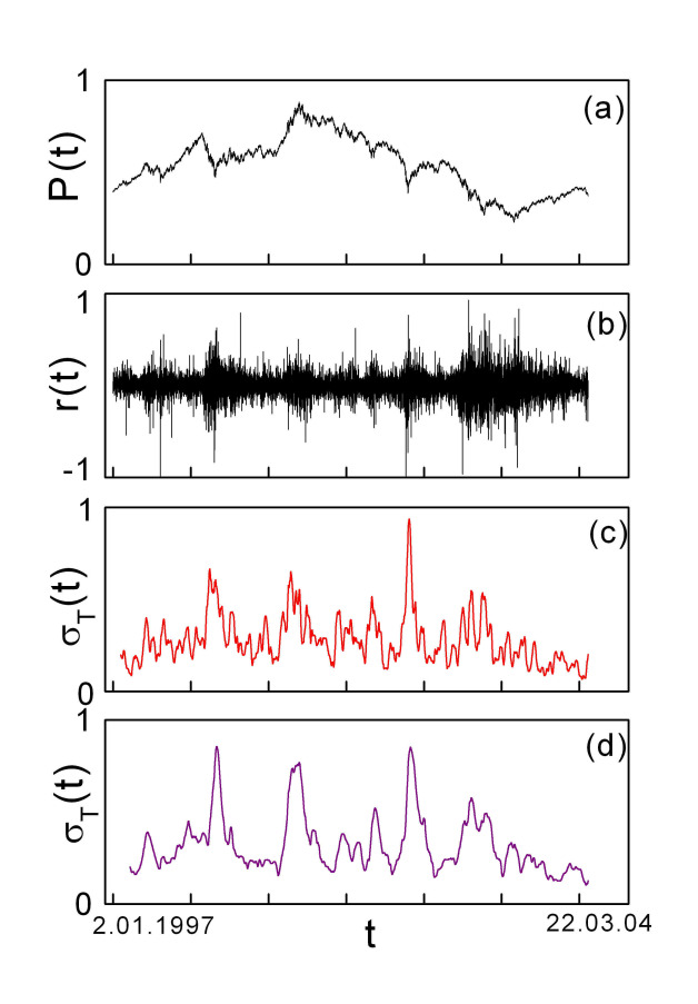
Figure 1: DAX stock index: (a) prices; (b) returns with $t^{\prime}=1h$; (c) volatility with $T=300h$; (d) volatility with $T=660h$.

Fig. 1 (b) shows the returns for $t^{\prime}=1h$. The volatility series are shown in Figs. 1 (c,d) respectively for $T=300h$ and $T=660h$. The Hurst exponents, calculated by the slope of the log-log plot of Eq. (2.7) as a function of $n$, are $H=0.50$ (return), $H=0.77$ (volatility $T=300h$) and $H=0.80$ (volatility $T=660h$). Fig. 2 shows the log-log plots of $C_{xx}(0)$ for the returns (squares) and volatility with $T=660$ (triangles). The scaling-law exhibited by the DAX series guarantees that its behaviour is a fractional Brownian motion. The function $C_{xy}(0)$ with $x=r(t)$ and $y=\sigma_{T}(t)$ with $T=660h$ is also plotted at varying $n$ in Fig. 2 (circles). From the slope of the log-log plot of $C_{xy}(0)$ vs $n$, one obtains $H=0.65$, i.e. the average between $H_{1}$ and $H_{2}$ as expected from Eq. (2.6).
Next, the cross-correlation is considered as a function of $\tau$. The plots of $C_{xy}(\tau)$ for $x=r(t)$ and $y=\sigma_{T}(t)$ with $T=300h$ and $T=660h$ are shown respectively in Fig. 3 (a,b) at different windows $n$.

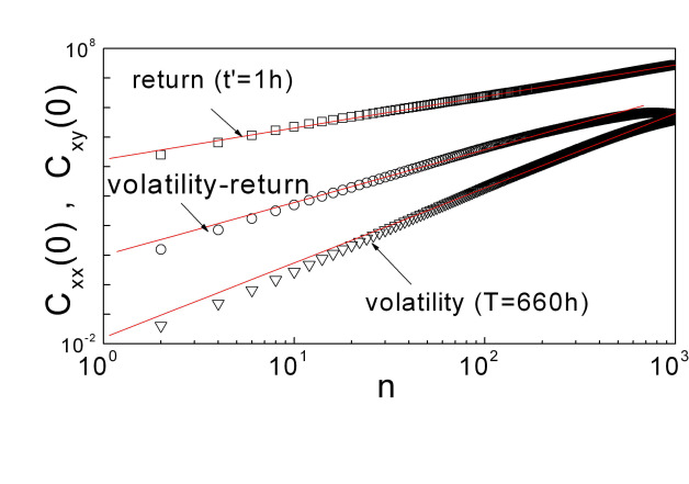
Figure 2: Log-log plot of $C_{xx}(0)$ for the DAX return (squares) and volatility (triangles) and of $C_{xy}(0)$ with $x=r(t)$ and $y=\sigma_{T}(t)$ (circles). Red lines are linear fits. The power-law behaviour is consistent with Eqs. (2.6,2.7).

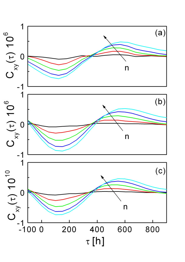
Figure 3: Cross-correlation $C_{xy}(\tau)$ with $x=r(t)$ and $y=\sigma_{T}(t)$ with (a) $T=300h$ and (b) $T=660h$; (c) with $x=r(t)$ and $y=\sigma_{T}(t)^{2}$ with $T=660h$. $n$ ranges from 100 to 500 with step 100.

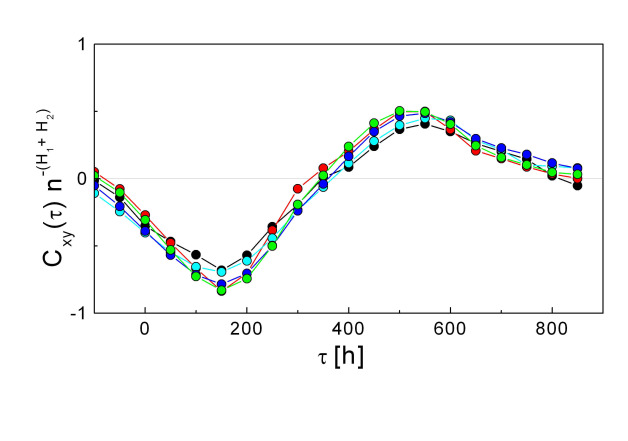
Figure 4: Plot of the function $C_{xy}(\tau)n^{-(H_{1}+H_{2})}$ with $x=r(t)$ and $y=\sigma_{T}(t)$ with $T=300h$. $H_{1}=0.5$ and $H_{2}=0.77$ $n$ ranges from 100 to 500 with step 100. One can note that the five curves collapse, within the numerical errors of the parameters entering the auto- and cross-corerlation functions. This is in accord with the invariance of the product $C_{xy}(\tau)n^{-(H_{1}+H_{2})}$ with the window $n$.

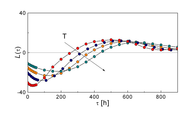
Figure 5: Leverage function with volatility windows $T$ = $100h$, $300h$, $660h$, $1000h$. The value of $n$ is $400$ equal for all the curves.

The function $C_{xy}(\tau)$ for $x=r(t)$ and $y=\sigma_{T}(t+\tau)^{2}$, is shown in Fig. 3(c). The cross-correlation takes negative values at small $\tau$ and reaches the minimum at about 10-12 days. This indicates that the volatility increases with negative returns (i.e. with price drops). Then $C_{xy}(\tau)$ changes sign relaxing asymptotically to zero from positive values at large $\tau$. The positive values of $C_{xy}(\tau)$ indicate that the volatility decreases when the returns become positive (i.e. when price rises) and are related to the restored equilibrium within the market (positive rebound days). It is worthy of remark that the (positive) maximum of the cross-correlation is always smaller than the (negative) minimum. This is the stylized fact known as down market effect. A relevant feature exhibited by the curves in Figs. 3 (a-c) is that the zeroes and the extremes of $C_{xy}(\tau)$ occur at the same values of $\tau$, which is consistent with wide-sense-stationarity for all the values of $n$. A further check of wide sense stationarity is provided by the plot of the function $C_{xy}(\tau)n^{-(H_{1}+H_{2})}$. In Fig. 4, $C_{xy}(\tau)n^{-(H_{1}+H_{2})}$ is plotted with $x=r(t)$ and $y=\sigma_{T}(t)$ with $T=300h$, $H_{1}=0.5$ and $H_{2}=0.77$, $n$ ranges from 100 to 500 with step 100. One can note that the five curves collapse in accord with the invariance of the product $C_{xy}(\tau)n^{-(H_{1}+H_{2})}$ with $n$.

In Fig. 5, the leverage correlation function $\mathcal{L}(\tau)=\langle\sigma_{T}(t+\tau)^{2}r(t)\rangle/\langle r(t)^{2}\rangle^{2}$ according to the definition put forward in [18], is plotted for different volatility windows $T$. The function $\langle\sigma_{T}(t+\tau)^{2}r(t)\rangle$ has been calculated by means of Eq.(2.1). The negative values of cross-correlation (at smaller $\tau$) and the following values (positive rebound days) at larger $\tau$ can be clearly observed for several volatility windows $T$. The function $\mathcal{L}(\tau)$ for the DAX stock index, estimated by means of the standard cross-correlation function, is shown in Figs. 1,2 of Ref. [20]. By comparing the curves shown in Fig. 5 to those of Ref. [20], one can note the higher resolution related to the possibility to detect the correlation at smaller lags (note the $\tau$ unit is hours, while in Ref.[18, 19, 20, 21] is days) and at varying windows $n$, implying the possibility to estimate the degree of cross-correlation at different frequencies. As a final remark, we mention that the cross correlation function between a fractional Brownian motion and its own width can be computed analytically in the large $n$ limit, following the derivation in the Appendix for two general fBm’s. The width of a fBm is one possible definition for the volatility, therefore the derivation in the Appendix provides a straightforward estimate of the leverage function.

3.2 Genomic Sequences

Several studies are being addressed to quantify cross-correlations among nucleotide position, intrinsic curvature and flexibility of the DNA helix, that may ultimately shed light on biological processes, such as protein targeting and transcriptional regulation [24, 25, 26]. One problem to overcome is the comparison of DNA fragments with di- and trinucleotide scales, hence the need of using high-precision numerical techniques. We consider deformability, stacking energy, propeller twist and position preference sequences of the Escherichia Coli chromosome. The sequences, with details about the methods used to synthetize/measure the structural properties, are available at the CBS database - Center for Biological Sequence Analysis of the Technical University of Denmark (http://www.cbs.dtu.dk/services/genomeAtlas/). In order to apply the proposed method, the average value is subtracted from the data, that are subsequently integrated to obtain the paths shown in Fig. 6. The series are $4938919bp$ long and have Hurst exponents: $H=0.70$ (deformability), $H=0.65$ (position preference), $H=0.73$ (stacking energy), $H=0.70$ (propeller twist).

The cross-correlation functions $C_{xy}(\tau)$ between deformability, stacking energy, propeller twist and position preference are shown in Fig. 7 (a-e). There is in general a remarkable cross-correlation along the DNA chain indicating the existence of interrelated patches of the structural and compositional parameters. The high correlation level between DNA flexibility measures and protein complexes indicates that the conformation adopted by the DNA bound to a protein depends on the inherent structural features of the DNA. It is worthy to remark that the present method provides the dependence of the coupling along the DNA chain rather than simply the values of the linear correlation coefficient $r$. In Table 4 of Ref. [26] one can find the following values of the correlation obtained by either numerical analysis or experimental measurements (in parentheses) over DNA fragments : (a) $r=-0.80~{}(-0.86)$; (b) $r=0.06~{}(0.00)$; (c) $r=-0.15~{}(-0.22)$; (d) $r=-0.74~{}(-0.82)$; (e) $r=-0.80~{}(-0.87)$. Moreover, also for the genomic sequences the function $C_{xy}(\tau)n^{-(H_{1}+H_{2})}$ is independent of $n$ within the numerical errors of the parameters entering the auto- and cross-correlation functions. In Fig. 8, $C_{xy}(\tau)n^{-(H_{1}+H_{2})}$ is shown for $x(t)$ the deformability, $y(t)$ the stacking energy, $H_{1}=0.7$ and $H_{2}=0.73$. $n$ ranges from 100 to 500 with step 100.

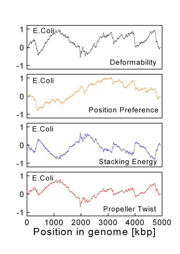
Figure 6: Structural sequences of the Escherichia Coli chromosome.

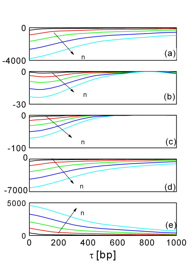
Figure 7: Cross-correlation $C_{xy}(\tau)$ between (a) deformability and stacking energy; (b) position preference and deformability (c) propeller twist and position preference; (d) propeller twist and stacking energy; (e) propeller twist and deformability. $n$ ranges from 100 to 500 with step 100.

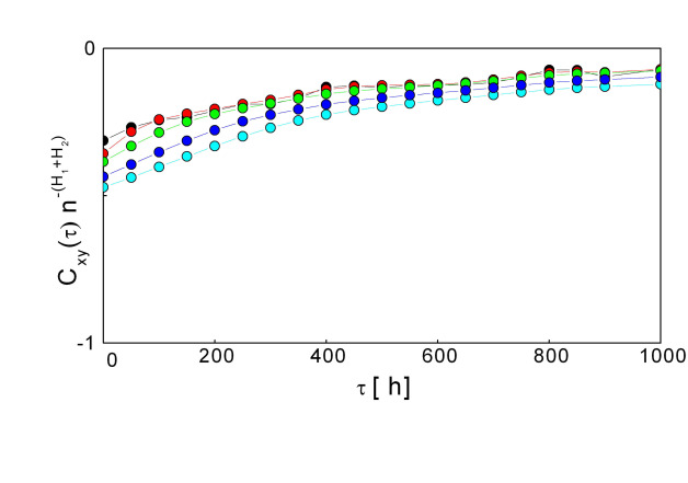
Figure 8: Plot of the function $C_{xy}(\tau)n^{-(H_{1}+H_{2})}$ with $x(t)$ the deformability, $y(t)$ the stacking energy, $H_{1}=0.7$ and $H_{2}=0.73$. $n$ ranges from 100 to 500 with step 100. One can note that the five curves collapse, within the numerical errors of the parameters entering the auto- and cross-corerlation functions. This is in in accord with the invariance of the product $C_{xy}(\tau)n^{-(H_{1}+H_{2})}$ with the window $n$.

4 Conclusions

A high-resolution, lag-dependent non-parametric technique based on Eqs. (2.1-2.3) to measure cross-correlation in long range-correlated series has been developed. The technique has been implemented on (i) financial returns and volatilities and (ii) structural properties of genomic sequences [35]. The results clearly show the existence of coupling regimes characterized by positive-negative feedback between the systems at different lags $\tau$ and windows $n$. We point out that - in principle - other methods might be generalized in order to yield estimates of the cross-correlation between long-range correlated series at varying $\tau$ and $n$. However, techniques operating over the series by means of a box division, such as DFA and R/S method, are a-priori excluded. The box division causes discontinuities in the sliding product of the two series at the extremes of each box, and ultimately incorrect estimates of the cross-correlation. The present method is not affected by this drawback, since Eqs. (2.1-2.3) do not require a box division.

Appendix A Details of the calculation:

Let us start from Eq. (2.4):

$$C_{xy}(t,\,\tau)=\Big{\langle}\big{[}B_{H_{1}}(t)-\widetilde{B}_{H_{1}}(t)\big{]}\big{[}B_{H_{2}}^{*}(t+\tau)-\widetilde{B}_{H_{2}}^{*}(t+\tau)\big{]}\Big{\rangle}\;\;\;,$$ (1.8)

that, after multiplying the terms in parentheses, becomes:

$$C_{xy}(t,\,t+\tau) =\Big{\langle}[B_{H_{1}}(t)B_{H_{2}}^{*}(t+\tau)-B_{H_{1}}(t)\widetilde{B}_{H_{2}}^{*}(t+\tau)$$ (1.9)

$$-\widetilde{B}_{H_{1}}(t)B_{H_{2}}^{*}(t+\tau)+\widetilde{B}_{H_{1}}(t)\widetilde{B}_{H_{2}}^{*}(t+\tau)]\Big{\rangle}\;\;\;.$$

In general, the moving average may be referred to any point of the moving window, a feature expressed by replacing Eqs. (2.2, 2.3) with

$$\tilde{x}_{n}(t)=\frac{1}{n}\sum_{k=-\theta n}^{n-\theta n}x(t-k)\qquad\quad\tilde{y}_{n}(t+\tau)=\frac{1}{n}\sum_{k=-\theta n}^{n-\theta n}y(t+\tau-k)$$ (1.10)

with $0\leq\theta\leq 1$. In the limit of $n\to\infty$, the sums can be replaced by integrals, so that:

$$\tilde{x}(t)=\int_{-\theta}^{1-\theta}x(\hat{t}-\hat{k})\qquad\quad\tilde{y}(t+\tau)=\int_{-\theta}^{1-\theta}y(\hat{t}+\hat{\tau}-\hat{k})$$ (1.11)

where $t=n\hat{t}$, $\tau=n\hat{\tau}$, $k=n\hat{k}$. For the sake of simplicity, the analytical derivation will be done by using the harmonizable representation of the fractional Brownian motion [36, 37, 39]:

$$B_{H}(t)\equiv\int_{-\infty}^{+\infty}\frac{e^{it\xi}-1}{|\xi|^{H+\frac{1}{2}}}d\bar{B}(\xi)\;,$$ (1.12)

where $d\bar{B}(\xi)$ is a representation of $dB(t)$ in the $\xi$ domain. In the following we will consider the case of $t>0$ and $t+\tau>0$. By using Eq. (1.12), the cross-correlation of two fbms $B_{H_{1}}(t)$ and $B_{H_{2}}(t+\tau)$ can be written as:

$$\langle B_{H_{1}}(t)B_{H_{2}}^{*}(t+\tau)\rangle=\Big{\langle}\int_{-\infty}^{+\infty}\frac{e^{it\xi}-1}{|\xi|^{H_{1}+\frac{1}{2}}}\,d\bar{B}(\xi)\,\int_{-\infty}^{+\infty}\frac{e^{-i(t+\tau)\eta}-1}{|\eta|^{H_{2}+\frac{1}{2}}}\,d\bar{B}(\eta)\Big{\rangle}\;.$$ (1.13)

Since $d\bar{B}$ is Gaussian, the following property holds for any $f,\,g\,\in\,L^{2}(\mathbb{R})$ :

$$\Big{\langle}\int_{-\infty}^{+\infty}f(\xi)d\bar{B}(\xi)\,\left(\int_{-\infty}^{+\infty}g(\eta)d\bar{B}(\eta)\right)^{*}\Big{\rangle}=\int_{-\infty}^{+\infty}f(\xi)g^{*}(\xi)\,d\xi$$ (1.14)

By using Eq. (1.14), after some algebra Eq. (1.13) writes:

$$\langle B_{H_{1}}(t)B_{H_{2}}^{*}(t+\tau)\rangle=D_{H_{1},\,H_{2}}\Big{(}t^{H_{1}+H_{2}}+(t+\tau)^{H_{1}+H_{2}}-|\tau|^{H_{1}+H_{2}}\Big{)}\;,\\$$ (1.15)

where $D_{H_{1},\,H_{2}}$ is a normalization factor which depends on $H_{1}$ and $H_{2}$. In the harmonizable representation of fBm, $D_{H_{1},\,H_{2}}$ takes the following form [38]:

$$D_{H_{1},\,H_{2}}=D_{H_{1}+H_{2}}=-\frac{2}{\pi}\cos\left[\frac{(H_{1}+H_{2})\pi}{2}\right]\Gamma[-(H_{1}+H_{2})]$$ (1.16)

normalized such that $D_{H_{1},\,H_{2}}=1$ when $H_{1}=H_{2}=\frac{1}{2}$. Different representations of the fBm lead to different values of the coefficient $D_{H_{1},\,H_{2}}$ [39, 40].

Eq. (1.15) can be used to calculate each of the four terms in the right hand side of Eq. (1.9). The mean value of each term in Eq. (1.9) is obtained from the general formula in Eq. (1.15); thus, substituting the right hand side of Eq. (1.15) and Eq. (1.11) into each term in Eq. (1.9) we obtain:

$$C_{xy}(\hat{t},\,\hat{\tau},\,\theta)=D_{H_{1},\,H_{2}}n^{H_{1}+H_{2}}\Big{[}\Big{(}\hat{t}^{H_{1}+H_{2}}+(\hat{t}+\hat{\tau})^{H_{1}+H_{2}}-|\hat{\tau}|^{H_{1}+H_{2}}\Big{)}$$

$$-\Big{(}\hat{t}^{H_{1}+H_{2}}+\int_{\hat{h}=-\theta}^{1-\theta}|\hat{t}-\hat{h}+\hat{\tau}|^{H_{1}+H_{2}}d\hat{h}-\int_{\hat{h}=-\theta}^{1-\theta}|\hat{t}-\hat{h}|^{H_{1}+H_{2}}d\hat{h}\Big{)}$$

$$-\Big{(}\int_{\hat{k}=-\theta}^{1-\theta}|\hat{t}-\hat{k}|^{H_{1}+H_{2}}d\hat{k}+(\hat{t}+\hat{\tau})^{H_{1}+H_{2}}-\int_{\hat{k}=-\theta}^{1-\theta}|\hat{t}+\hat{k}|^{H_{1}+H_{2}}d\hat{k}\Big{)}$$

$$+\Big{(}\int_{\hat{k}=-\theta}^{1-\theta}|\hat{t}-\hat{k}|^{H_{1}+H_{2}}d\hat{k}+\int_{\hat{h}=-\theta}^{1-\theta}|\hat{t}-\hat{h}+\hat{\tau}|^{H_{1}+H_{2}}d\hat{h}$$

$$-\int_{\hat{h}=-\theta}^{1-\theta}\int_{\hat{k}=-\theta}^{1-\theta}|\hat{\tau}-\hat{h}-\hat{k}|^{H_{1}+H_{2}}d\hat{h}\,d\hat{k}\Big{)}\Big{]}$$ (1.17)

where each term in round parentheses corresponds to each of the four terms in Eq. (1.9). Summing the terms in Eq. (A), one can notice that time $t$ cancels out, thus one finally obtains:

$$C_{xy}(\hat{\tau},\,\theta) =n^{H_{1}+H_{2}}D_{H_{1},\,H_{2}}\Big{[}-\hat{\tau}^{H_{1}+H_{2}}+\int_{-\theta}^{1-\theta}|\hat{\tau}-\hat{h}|^{H_{1}+H_{2}}\,d\hat{h}$$

$$+\int_{-\theta}^{1-\theta}|\hat{\tau}+\hat{k}|^{H_{1}+H_{2}}\,d\hat{k}-\int_{-\theta}^{1-\theta}|\hat{\tau}-\hat{h}+\hat{k}|^{H_{1}+H_{2}}\,d\hat{h}\,d\hat{k}\;\Big{]}\;,$$

Consistently with the large $n$ limit, we take $\tau<n$, namely $\hat{\tau}<1$. The integral (A) admits four different solutions, depending on the values taken by the parameters $\hat{\tau}$ and $\theta$. Let us consider each case separately.

Case 1: $\hat{\tau}<\theta$ and $\hat{\tau}+\theta<1$

$$C_{xy}(\hat{\tau},\,\theta) =n^{H_{1}+H_{2}}D_{H_{1},\,H_{2}}\Big{[}-\hat{\tau}^{H_{1}+H_{2}}-\frac{(1-\hat{\tau})^{2+H_{1}+H_{2}}-2\hat{\tau}^{2+H_{1}+H_{2}}+(1+\hat{\tau})^{2+H_{1}+H_{2}}}{(1+H_{1}+H_{2})(2+H_{1}+H_{2})}$$

$$+\frac{(1+\hat{\tau}-\theta)^{1+H_{1}+H_{2}}+(\theta-\hat{\tau})^{1+H_{1}+H_{2}}+(1-\hat{\tau}-\theta)^{1+H_{1}+H_{2}}+(\hat{\tau}+\theta)^{1+H_{1}+H_{2}}}{1+H_{1}+H_{2}}\Big{]}$$

Case 2: $\hat{\tau}<\theta$ and $\hat{\tau}+\theta>1$

$$C_{xy}(\hat{\tau},\,\theta) =n^{H_{1}+H_{2}}D_{H_{1},\,H_{2}}\Big{[}-\hat{\tau}^{H_{1}+H_{2}}-\frac{(1-\hat{\tau})^{2+H_{1}+H_{2}}-2\hat{\tau}^{2+H_{1}+H_{2}}+(1+\hat{\tau})^{2+H_{1}+H_{2}}}{(1+H_{1}+H_{2})(2+H_{1}+H_{2})}$$

$$+\frac{(1+\hat{\tau}-\theta)^{1+H_{1}+H_{2}}+(\theta-\hat{\tau})^{1+H_{1}+H_{2}}-(\hat{\tau}+\theta-1)^{1+H_{1}+H_{2}}+(\hat{\tau}+\theta)^{1+H_{1}+H_{2}}}{1+H_{1}+H_{2}}\Big{]}$$

Case 3: $\hat{\tau}>\theta$ and $\hat{\tau}+\theta<1$

$$C_{xy}(\hat{\tau},\,\theta) =n^{H_{1}+H_{2}}D_{H_{1},\,H_{2}}\Big{[}-\hat{\tau}^{H_{1}+H_{2}}-\frac{(1-\hat{\tau})^{2+H_{1}+H_{2}}-2\hat{\tau}^{2+H_{1}+H_{2}}+(1+\hat{\tau})^{2+H_{1}+H_{2}}}{(1+H_{1}+H_{2})(2+H_{1}+H_{2})}$$

$$+\frac{(1+\hat{\tau}-\theta)^{1+H_{1}+H_{2}}-(\hat{\tau}-\theta)^{1+H_{1}+H_{2}}+(1-\hat{\tau}-\theta)^{1+H_{1}+H_{2}}+(\hat{\tau}+\theta)^{1+H_{1}+H_{2}}}{1+H_{1}+H_{2}}\Big{]}$$

It is easy to see that this case includes the Eq. (2.5) treated in the paper.

Case 4: $\hat{\tau}>\theta$ and $\hat{\tau}+\theta>1$

$$C_{xy}(\hat{\tau},\,\theta) =n^{H_{1}+H_{2}}D_{H_{1},\,H_{2}}\Big{[}-\hat{\tau}^{H_{1}+H_{2}}-\frac{(1-\hat{\tau})^{2+H_{1}+H_{2}}-2\hat{\tau}^{2+H_{1}+H_{2}}+(1+\hat{\tau})^{2+H_{1}+H_{2}}}{(1+H_{1}+H_{2})(2+H_{1}+H_{2})}$$

$$+\frac{(1+\hat{\tau}-\theta)^{1+H_{1}+H_{2}}-(\hat{\tau}-\theta)^{1+H_{1}+H_{2}}-(\hat{\tau}+\theta-1)^{1+H_{1}+H_{2}}+(\hat{\tau}+\theta)^{1+H_{1}+H_{2}}}{1+H_{1}+H_{2}}\Big{]}$$

References

References

- [1] M. Rosenblum and A. Pikovsky, (2007) Phys. Rev. Lett. 98, 064101.
- [2] T. Zhou, L. Chen and K. Aihara, (2005) Phys. Rev. Lett. 95, 178103.
- [3] S. Oberholzer et al. (2006) Phys. Rev. Lett. 96, 046804.
- [4] M. Dhamala, G. Rangarajan, (2008) M. Ding, Phys. Rev. Lett. 100, 018701.
- [5] P. F. Verdes, (2005) Phys. Rev. E 72, 026222.
- [6] M. Palus and M. Vejmelka, (2007) Phys. Rev. E 75, 056211.
- [7] T. Kreuz et al. (2007) Physica D 225, 29 .
- [8] Lu-Chun Du and Dong-Cheng Mei, (2008) J. Stat. Mech. P11020.
- [9] P. Tass et al. (1998) Phys. Rev. Lett. 81, 3291.
- [10] P. Huybers, (2006) W. Curry, Nature 441, 7091.
- [11] Y. Ashkenazy, (2006) Climate Dynamics 27, 421.
- [12] F. Black, (1976) J. of Fin. Econ. 3, 167.
- [13] W. Schwert, J. of Finance (1989) 44, 1115.
- [14] R. Haugen, E. Talmor, W. Torous, (1991) J. of Finance 44, 1115.
- [15] L. Glosten, J. Ravi and D. Runkle, (1992) J. of Finance 48, 1779.
- [16] G. Bekaert, G. Wu, (2000) The Review of Financial Studies 13, 1.
- [17] S. Figlewski, X. Wang (2000) Is the ’Leverage Effect’ a Leverage Effect? , Working Paper, Stern School of Business, New York.
- [18] J. P. Bouchaud, A. Matacz and M. Potters, (2001) Phys. Rev. Lett. 87, 228701.
- [19] J. Perello and J. Masoliver, (2003) Phys. Rev. E 67, 037102.
- [20] T. Qiu, B. Zheng, F. Ren and S. Trimper, (2006) Phys. Rev. E 73, 065103(R).
- [21] R. Donangelo, M. H. Jensen, I. Simonsen, K. Sneppen, (2006) J. Stat. Mech. L11001.
- [22] I Varga-Haszonits and I Kondor, (2008) J. Stat. Mech. P12007.
- [23] M. Montero, (2007) J. Stat. Mech. P04002.
- [24] J. Moukhtar, E. Fontaine, C. Faivre-Moskalenko and A. Arneodo, (2007) Phys. Rev. Lett. 98, 178101.
- [25] T.E. Allen, N.D. Price, A. Joyce and B.O. Palsson, (2006) PLoS Computational Biology, 2, e2.
- [26] A.G. Pedersen, L.J. Jensen, S. Brunk, H.H. Staerfeld and D.W. Ussery, (2000) J. Mol. Biol. 299, 907.
- [27] W.C. Jun, G. Oh and S. Kim, (2006) Phys. Rev. E 73, 066128.
- [28] B. Podobnik, H.E. Stanley, (2008) Phys. Rev. Lett. 100, 084102.
- [29] B. B. Mandelbrot, J. W. Van Ness, (1968) SIAM Rev. 4, 422.
- [30] A. Carbone, G. Castelli, H. E. Stanley, Phys. Rev. E 69, 026105 (2004).
- [31] A. Carbone, Phys. Rev. E 76, 056703 (2007).
- [32] S. Arianos and A. Carbone, Physica A 382, 9 (2007).
- [33] A. Carbone and H. E. Stanley, Physica A 384, 21 (2007).
- [34] A. Carbone and H. E. Stanley, Physica A 340, 544 (2004).
- [35] The MATLAB and C++ codes implementing the proposed method, the DAX and E-COLI sequences used in this work are downloadable at: www.polito.it/noiselab/utilities
- [36] A. Benassi, S. Jaffard, D. Roux, Rev. Mat. Iber. 13, 19, (1997).
- [37] S. Cohen, Fractals: Theory and Applications in Engineering. M. Dekking, J. Lévy Véhel, E. Lutton and C. Tricot (Eds.). Springer Verlag, 1999.
- [38] A. Ayache, S. Cohen, J. Levy Vehel, Proceedings of the conference ICASSP, Istanbul June 2000.
- [39] V. Dobric, F. M. Ojeda, IMS Lecture Notes-Monograph Series, High Dimensional Probability, 51, 77, (2006).
- [40] S. A. Stoev, M. S. Taqqu, Stochastic Processes and their Applications 116, 200 (2006).