Proposal of an explanation of the Pioneer anomaly

Abstract

We propose here an explanation of the Pioneer anomaly that is not in conflict with the cartography of the solar system. In our model, the spaceship does not suffer any extra acceleration but follows the trajectory predicted by standard gravitational theory. The observed acceleration is not real but apparent and has the same observational footprint as a deceleration of astronomical time with respect to atomic time. The details can be summarized as follows: i) as we argued in a recent paper, there is an unavoidable coupling between the background gravitation that pervades the universe and the quantum vacuum because of the long range and universality of gravity; ii) via the fourth Heisenberg relation, we show that this coupling causes a progressive desynchronization of the astronomical and atomic clock-times, in such a way that the former decelerates adiabatically with respect to the latter; and iii) since gravitational theory uses astronomical time and the observers use atomic time (they are using devices based on quantum physics), this desynchronization necessarily causes a discrepancy between theory and observation, so that the observed velocity of the spaceship is smaller than the predicted one, in such a way that the Pioneer seems to lag behind its expected position. The discoverers of the anomaly suggested “the possibility that the origin of the anomalous signal is new physics” although they added “the most likely cause of the effect is an unknown systematics,” but also that “In the unlikely event that there is new physics, one does not want to miss it because one had the wrong mind set.”

Keywords: Time, quantum vacuum, background gravity, Pioneer anomaly.

I The Pioneer anomaly

This paper proposes a solution to the Pioneer anomaly that is not in conflict with the cartography of the solar system, which is up to now the most serious obstacle to the explanation of this riddle. It is based on a previous paper by us, in which we show that the coupling of the quantum vacuum and the background gravitation of the entire universe must cause a desynchronization of the astronomical and the atomic clocks that has the same observational fingerprint as the Pioneer anomaly RT08 ; Ran03 .

This intriguing phenomenon, discovered in 1980 and reported in 1998 by Anderson et al. And98 ; And02 , consists of an adiabatic frequency blue drift of the two-way radio signals from the Pioneer 10 and 11 (launched in 1972 and 1973), manifest in a residual Doppler shift that increases linearly with time as

$$\dot{\nu}/\nu=2a_{\rm t}\,,\quad\mbox{or}\quad\nu=\nu_{0}\,[1+2a_{\rm t}(t-t_{0})]\,,$$ (1)

where $t_{0}$ is the launch time and $2a_{\rm t}=(5.82\pm 0.88)\times 10^{-18}\mbox{ s}^{-1}\simeq(2.53\pm 0.38)H_{0}$, $H_{0}$ being the Hubble constant (overdot means time derivative). Many years after its discovery, the phenomenon is still unexplained. As the discoverers themselves explain “At that time [1980] the navigation data had already indicated the presence of an anomaly in the Doppler data; but at first the anomaly was only considered to be an interesting navigational curiosity and was not seriously analyzed Mar04 ”.

It must be stressed that the signal found by Anderson et al. is very well-defined. Because of its linearity, the residual frequency $\nu$ of the ship appears as a straight line in a plot ($\nu,\,t$) And98 . This strongly suggests that the anomaly is the evidence of a new effect, probably with a cosmological origin, so that the curve $\nu(t)$ can be accurately approximated by its tangent for a scale of just a few decades. This contrasts with some attempts to explain the effect as a local solar system phenomenon Lam05 ; Rat06 . In 1998, after many attempts to explain the effect, the discoverers admitted “the possibility that the origin of the anomalous signal is new physics” And98 , a suggestion reiterated four years later in reference And02b . But in the conclusions of reference And02 (and in several other texts where they repeat the same idea) they say with a pinch of caution “Currently, we find no mechanism or theory that explains the anomalous acceleration … Until more is known, we must admit that the most likely cause of the effect is an unknown systematics.” Consequently, they performed new analysis of the data Tur06 , but they end their conclusions with this statement: “In the unlikely event that there is new physics, one does not want to miss it because one had the wrong mind set” (see also Nie07 ).

I.1 A first interpretation of the effect

Since it was detected as a Doppler shift that does not correspond to any known motion of the spaceship, the simplest interpretation is that there is an anomalous constant acceleration towards the Sun. However, this is not acceptable since it would conflict with the well-known cartography of the solar system and with the equivalence principle.

Indeed, any interpretation of the anomaly in terms of a real, if unmodelled, acceleration, due to a real force acting on the spaceship, would face serious problems. Just as a simple example, the assumption that the acceleration culprit is a distribution of dark matter around the Sun with density $\rho\propto A/r$ and a particular value of $A$, gives the right value of the Pioneer acceleration for all the bodies in the solar system. However, this would imply too much mass and would predict an unacceptable variation in the perihelion of the planets, increasing with the distance to the Sun. In fact, to explain the anomaly without affecting the very well known cartography of the solar system is probably the most serious difficulty to solve the riddle. Anderson et al. included the following paragraph in references And98 p. 2860 and And02 p 41:

“The anomalous acceleration is too large to have gone undetected in planetary orbits, particularly for Earth and Mars. NASA’s Viking Mission provided radio-ranging measurements to an accuracy of 12 m. If a planet experiences a small anomalous radial acceleration $a_{\sc A}$, its orbital radius is perturbed by

$$\Delta r=-{\ell^{\,6}a_{\sc A}\over(GM_{\odot})^{4}}\rightarrow-{ra_{\sc A}\over a_{\sc N}},$$ (2)

where $\ell$ is the orbital angular momentum per unit mass and $a_{\sc N}$ is the Newtonian acceleration at $r$. [The right value in eq (2) holds in the circular orbit limit.]

For Earth and Mars, this is about $-21$ km and $-76$ km. However, the Viking data determine the difference between Earth and Mars orbital radii to about 100 m accuracy and the sum to an accuracy of 150 m. The Pioneer effect is not seen [as it should be].”

In other words, the cartography of the solar system would be affected in an unacceptable way. However, it must be underscored that this irreproachable argument by Anderson et al. assumes as a necessary condition that the Pioneer effect is an anomalous but real acceleration, due to a real force therefore (the previous value of $\Delta r$ is calculated by adding $-a_{\rm A}$ to the RHS of the planets’ radial equations of motion). If this is not so, the conclusion is not necessarily right and the effect does not necessarily include a negative correction to the radii of the orbits.

This has motivated many to look for an unknown systematic error affecting the observations and has contributed to extending a misunderstanding: that it is not possible to solve the riddle without affecting the well-known solar system data. This is also the reason for the change in the name of the effect from “Pioneer acceleration” to “Pioneer anomaly.”

We interpret all this as a compelling indication that the solution will be found with a model in which the Pioneer acceleration is not real but only apparent. This is the case for our proposal. As will be shown in the following, the Pioneer follows, according to this work, the trajectory predicted by the standard gravitation theory without any extra acceleration. Or, more precisely, the anomaly is not a real effect in our model, but just an observational effect caused by the discrepancy between the astronomical and atomic clock-times. It is, therefore, free from this contradiction.

I.2 A second interpretation of the effect

Because of the previous problems, Anderson et al. then attempted a second interpretation: $a_{\rm t}$ would be “a clock acceleration”, expressing a kind of non-homogeneity of time And98 . They imagined it in an intuitive and phenomenological way, without theoretical reasons, explaining that, in order to fit the trajectory, “we were motivated to try to think of any (purely phenomenological) ‘time’ distortions that might fortuitously fit the Pioneer results” (our emphasis, ref. And02 , section XI-D). In particular, they added various quadratic terms to the time, obtaining thus better fits to the trajectory. In one, which they call “Quadratic time augmentation model” they add to the TAI-ET (International Atomic Time-Ephemeris Time) transformation the following distortion of the ephemeris time ET

$$\mbox{ET}\rightarrow\mbox{ET}^{\prime}=\mbox{ET}+{1\over 2}\,a_{\rm ET}\,\mbox{ET}^{2}\,,$$ (3)

where $a_{\rm ET}$ is an inverse time. In the “Quadratic in time model” which they qualify as “especially fascinating”, they add a quadratic in time term to the light time as seen by a DSN station, so that

$$\Delta\mbox{TAI} = \mbox{TAI}_{\rm received}-\mbox{TAI}_{\rm sent}$$

$$\rightarrow \Delta\mbox{TAI}^{\prime}=\Delta\mbox{TAI}+{1\over 2}\,a_{\rm quad}(\mbox{TAI}_{\rm received}^{2}-\mbox{TAI}_{\rm sent}^{2}).$$

Note that to add quadratic terms is similar to introducing desynchronizations or accelerations so that the times they use are replaced by other differently defined times that accelerate with respect to them. But they later gave up this idea because of the lack of any theoretical basis and due to contradictions with the determination process of the orbits.

I.3 Our model

We argue here that the Pioneer anomaly is not a problem of systematics or of data handling but a genuine new effect, an indication in fact that we lack some important theoretical concepts. More precisely, we show here that the anomaly has the same observational signature as the desynchronization of the atomic and the astronomical clocks caused by the coupling between the background gravitational potential and the quantum vacuum, a new phenomenon studied in RT08 , where the reader is referred to for details (see also Ran03 ).

In order to understand the meaning of the preceding sentence, let us consider, as a simple illustrative example, the case in which an observer has two different clocks that measure two times $t_{1}$ and $t_{2}$, which accelerate adiabatically with respect to one another so that ${\rm d}t_{2}/{\rm d}t_{1}=1+A(t-t_{0})$, where $A={\rm d}^{2}t_{2}/{\rm d}t_{1}^{2}$ is a small inverse time and $t_{0}$ an initial time. Note that it is not necessary to specify the kind of time in the RHS at first order. The clocks are non-equivalent because the second derivative $A$ is non-zero. The observer measures the velocity of the particle with the two times, placing a series of synchronized clocks of each kind along the particle trajectory and observing the mark on the clocks when the position of the particle coincide with that of each particular clock. He will thus find the relation $v_{2}=v_{1}[1+A(t-t_{0})]$, where the subindexes indicate the time used to measure $v$. He would find the same effect on the frequency of any spectroscopic line or even for the light speed, so that $c_{2}=c_{1}[1+A(t-t_{0})]$ and $\nu_{2}=\nu_{1}[1+A(t-t_{0})]$ (compare with (1)). If he were unaware of the non equivalence of $t_{1}$ and $t_{2}$, he would be surprised and would look for some error in his measurement method (as a note of historical interest, we may mention Milne’s ideas which, on cosmological grounds, suggest the possible existence of different time scales Mil37 ; Mil40 ).

In spite of this simple example, all this may sound strange, but note that it is improbable that the anomaly will involve only known physics, considering that it remains unexplained more than 25 years after its discovery. In other words, it would seem strange that, when the solution of the riddle will be found, it would not seem strange. To end this introductory section, it must be underscored that, although the present model is based on new physical ideas, it does not conflict with any established law or principle.

II The coupling background gravity – quantum vacuum and the desynchronization of the astronomical and the atomic clocks

In a previous recent paper RT08 , we analyzed the idea of a coupling between the background potential that pervades the universe and the quantum vacuum, an obligatory effect due to the universality and long range of gravitation. Building on the fourth Heisenberg relation, we found that such a coupling would cause a discrepancy between the two main clock-times of physics. The astronomical clock-time, say $t_{\rm astr}$, is defined by the trajectories of the planets and other celestial bodies, while the atomic clock-time, say $t_{\rm atomic}$, is founded on the oscillations of atomic systems. The former is measured with classical and gravitational clocks, the solar system for instance, while the latter is determined using quantum and electromagnetic systems as clocks, in particular the oscillations of atoms or masers. Contrary to the implicit tradition, these two times could be different in principle since they are based on different physical laws. They could be ticking at different rates, even when located at the same place and having the same velocity. They are certainly almost equal, at least at small scales, but since we lack a unified theory of gravitation and quantum physics, the assumption that they are exactly the same $t_{\rm astr}=t_{\rm atomic}$ must not be accepted a priori without discussion. In this work, the march of the latter with respect to the former is defined as the derivative $u={\rm d}t_{\rm atomic}/{\rm d}t_{\rm astr}$.

To make this paper as self-contained as possible, here we will briefly summarize the main results of our previous paper RT08 (see also Ran03 . It is evident that the physics of the quantum vacuum is important because it fixes the values of some observable quantities and gives rise to observable phenomena. Probably its importance will increase during next decades. We are interested in the sea of virtual electron-positron pairs that pop-up and disappear constantly in empty space with their charges and spins. On the average, speaking phenomenologically, a virtual pair created with energy $E$ lives during a time $\tau_{0}=\hbar/E$, according to the fourth Heisenberg relation. This has an important consequence: the optical density of empty space must depend on the gravitational field. Indeed, if $\Psi$ is the averaged dimensionless gravitational potential, i. e. the potential of all the mass-energy in the entire universe assuming that it is uniformly distributed, the pairs have an extra energy $E\Psi$, so that their lifetime and number density must depend on $\Psi$ as

$$\tau_{\Psi}=\hbar/(E+E\Psi)=\tau_{0}/(1+\Psi);\qquad{\cal N}_{\Psi}={\cal N}_{0}/(1+\Psi),$$ (5)

RT08 . If $\Psi$ decreases, the quantum vacuum becomes denser, since the density of charges and spins becomes higher; if $\Psi$ increases, the quantum vacuum becomes thinner. In an expanding universe, the background potential is time dependant $\Psi=\Psi(t)$ and increases secularly and adiabatically so that its time derivative is positive at present time $\dot{\Psi}_{0}>0$ and small, probably of order $H_{0}$. It must be stressed that this is not an ad hoc hypothesis, but a necessary consequence of the fourth Heisenberg relation and of the universality of gravitation.

Let us take the Newtonian approximation and accept then the following phenomenological hypothesis: the quantum vacuum can be considered as a substratum, a transparent optical medium characterized by a relative permittivity $\varepsilon_{\rm r}(\Psi)$ and a relative permeability $\mu_{\rm r}(\Psi)$, which are decreasing functions of $\Psi(t)$. As $\Psi(t)$ increases, the optical density of the medium decreases (since there are less charges and spins) and vice versa. As presented in previous work, we express, at first order in the variation of $\Psi(t)$ and near present time $t_{0}$, the permittivity and the permeability of empty space as $\varepsilon=\varepsilon_{0}\varepsilon_{\rm r}(t)=\varepsilon_{0}\{1-\beta[\Psi(t)-\Psi(t_{0})]\}$, $\mu=\mu_{0}\mu_{\rm r}(t)=\mu_{0}\{1-\gamma[\Psi(t)-\Psi(t_{0})]\}$ where $\beta$ and $\gamma$ are certain coefficients, necessarily positive since the quantum vacuum must be dielectric but paramagnetic. The results of this paper will depend only on the semisum $\eta=(\beta+\gamma)/2$. It will be seen in the following that the time $t$ is an astronomical time, as is the ephemeris time, so that we will note it as $t_{\rm astr}\,(=t)$ from now on.

It was shown in former work Ran03 that, if the permittivity and the permeability vary adiabatically with time, the frequency and the speed of an electromagnetic wave obey $\dot{\nu}/\nu=\dot{c}/c=-(\dot{\varepsilon}/\varepsilon+\dot{\mu}/\mu)/2=\eta\dot{\Psi}_{0}$ (overdot means derivative with respect $t_{\rm astr}$), if they are defined with respect to $t_{\rm astr}$, so that near present time (or launch time) $t_{\rm astr,\,0}$

$$\nu_{\rm astr}=\nu_{\rm astr,\,0}[1+a(t_{\rm astr}-t_{\rm astr,\,0})]\,;\qquad c_{\rm astr}=c[1+a(t_{\rm astr}-t_{\rm astr,\,0})]\,,$$ (6)

with $a=\eta\dot{\Psi}_{0}\,(>0)$. If $a$ is very small, these variations are adiabatic. The sub-index “astr” indicates that the corresponding quantity has been defined or measured using astronomical time $t_{\rm astr}$ and where $c$ is the standard value of the light speed, the quantity that appears in the tables of physical constants. We see that both the frequency and the light speed increase adiabatically with time $t_{\rm astr}$. In order to describe this situation, we define a refractive index $n(t)=1+a(t_{\rm astr}-t_{\rm astr},\,0)$. However, $\nu$ and $c$ are constant if defined with the time $t_{\rm atomic}$, determined by the relation

$${\rm d}t_{\rm atomic}=[1+a(t_{\rm astr}-t_{\rm astr,\,0})]\,{\rm d}t_{\rm astr}=n(t_{\rm astr}){\rm d}t_{\rm astr}\,.$$ (7)

It is clear that $t_{\rm atomic}$ is the time measured by the atomic clocks, since the periods of the atomic oscillations are obviously constant with respect to them. In fact they are their basic units. The light speed is thus a universal constant, as it must be, if defined with respect to $t_{\rm atomic}$. Note that the derivatives with respect to the two clock-times are equal at present time $t_{\rm astr,\,0}$ because ${\rm d}t_{\rm atomic}/{\rm d}t_{\rm astr}=1$ at that instant. Hence, we can keep the same symbol for these two derivatives ${\rm d}\Psi/{\rm d}t_{\rm astr}={\rm d}\Psi/{\rm d}t_{\rm atomic}=\dot{\Psi}_{0}$. Since $\dot{\Psi}_{0}>0$ then $a>0$, so that the march of the atomic clocks with respect to the astronomical ones is equal to $u={\rm d}_{\rm atomic}/{\rm d}t_{{}_{\rm astr}}=1+a(t_{\rm astr}-t_{\rm astr,\,0})>1$ for $t_{\rm astr}>t_{\rm astr,\,0}$. Note also that the refractive index $n$ is equal to the march $u$.

All this shows that the effect of the quantum vacuum would be to desynchronize the astronomical and the atomic clocks in such a way that the former decelerates adiabatically with respect to the latter. As a consequence, the light speed and the frequencies would increase progressively if they are measured with the astronomical time $t_{\rm astr}$. However they are constant if measured with the atomic time $t_{\rm atomic}$. Synchronizing the two times and taking the international second as their common basic unit at present time (or at launch time), so that $t_{\rm astr,\,0}=t_{\rm atomic,\,0}=t_{0}=0$, then ${\rm d}t_{\rm astr}={\rm d}t_{\rm atomic}$ (ref. RT08 ).

It follows from (7) that, if $t_{0}=0$,

$$t_{\rm astr}=t_{\rm atomic}-{1\over 2}\,a\,t_{\rm atomic}^{2}\qquad\mbox{ and }\qquad{\!\!{\rm d}^{2}t_{\rm astr}\over{\rm d}t_{\rm atomic}^{2}}=-\eta\dot{\Psi}_{0}=-a\,.$$ (8)

There is a striking similarity between (8) and (3)-(I.2), which could explain why Anderson et al. obtained improved data fits by introducing these time distortions. As can be seen, the quantity $a=\eta\dot{\Psi}_{0}$ in our model corresponds to $2a_{\rm t}$ in the papers by Anderson et al., which shows that it is $a$ or $2a_{\rm t}$, not $a_{\rm t}$, which truly deserves the name of “clock acceleration”.

If the march $u={\rm d}t_{\rm atomic}/{\rm d}t_{\rm astr}=1+a(t_{\rm astr}-t_{\rm astr,\,0})$ is not constant, the two clock-times are not equivalent, so that the speed measured using the Doppler effect with devices sensitive to the quantum time, say $v_{\rm atomic}={\rm d}\ell/{\rm d}t_{\rm atomic}$, would be different from the astronomical speed $v_{\rm astr}={\rm d}\ell/{\rm d}t_{\rm astr}$. Indeed

$$v_{\rm atomic}=v_{\rm astr}/u=v_{\rm astr}[1-a(t_{\rm astr}-t_{\rm astr,\,0})]\,,$$ (9)

and the frequencies obey the same relation $\nu_{\rm atomic}=\nu_{\rm astr}[1-a(t_{\rm astr}-t_{\rm astr,\,0})]$. Since gravitational theory gives $v_{\rm astr}$ while the observers measure $v_{\rm atomic}$, there must be a discrepancy between theory and observation. In this way, an apparent but unreal violation of standard gravity would be detected.

III Explanation of the anomaly

These arguments give a compelling explanation of the anomaly as an effect of the discrepancy between these two times. Let us see why. The frequencies measured by Anderson et al. are standard frequencies defined with respect to atomic time $t_{\rm atomic}$, since they observe them with devices based on quantum physics. They did not measure frequencies with respect to the astronomical time. However, since (i) the trajectory was determined by standard gravitational theory that use astronomical time and (ii) the observed frequency shifts used atomic time, they found a discrepancy between theory and observation: this is the Pioneer Anomaly.

Once all this is accepted, the anomaly is easily explained. To do that, we will now follow two paths, both very simple: first a more intuitive and geometrical explanation, and second a more precise and formal account. The first starts with the distance traveled by a spaceship along a given trajectory, which can be expressed in two forms

$$d=\int_{0}^{t_{\rm atomic}}\!\!\!\!\!\!\!\!v_{\rm atomic}(t^{\prime}){\rm d}t^{\prime}=\int_{0}^{t_{\rm astr}}\!\!\!\!\!v_{\rm astr}(t^{\prime})\,{\rm d}t^{\prime}\,,$$ (10)

where $t^{\prime}=t_{\rm atomic}$ in the first integral, $t^{\prime}=t_{\rm astr}$ in the second and $(0,t_{\rm atomic})$ and $(0,t_{\rm astr})$ are the same time interval expressed with the two times (because $v_{\rm atomic}=v_{\rm astr}/u$ and ${\rm d}t_{\rm atomic}=u{\rm d}t_{\rm astr}$). Equation (10) is always valid, whether or not the two times are equal. What we are proposing as the solution to the riddle is that the two times are in fact different. If, however, they are assumed to be equal $t_{\rm astr}=t_{\rm atomic}$, then the distance deduced from observations $d_{\rm observ}$ and the expected distance according to standard gravitational theory $d_{\rm theory}$ up to the same $t_{\rm atomic}$, which are

$$d_{\rm observ} = \int_{0}^{t_{\rm atomic}}\!\!\!\!\!\!\!\!\!\!\!\!v_{\rm atomic}(t^{\prime})\,{\rm d}t^{\prime}\,,\quad d_{\rm theory}=\int_{0}^{t_{\rm atomic}}\!\!\!\!\!\!\!\!\!v_{\rm astr}(t^{\prime})\,{\rm d}t^{\prime}\,,$$

with $t^{\prime}=t_{\rm atomic}$ in both integrals, would be different. Now, if $u>1$ as it was during the Pioneer flight, the atomic velocity is smaller so that $d_{\rm observ}<d_{\rm theory}$: it would seem that the ship travels a smaller than expected distance. Apparently, it would lag behind the predicted position.

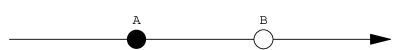
Figure 1: Schematic representation with arbitrary units of the Pioneer anomaly (explanation in the text.)

All this is explained in Figure 1, where the Pioneer trajectory receding from the Sun is plotted schematically. The spacecraft moves in the direction of the arrow. The white circle at $B$ is the position of the ship according to standard gravitation, its real position in fact if this theory is correct. The black circle at $A$ is the apparent position, deduced from the ship’s velocity after measuring the Doppler effect on the frequencies of the signals using atomic clocks and devices. If the two times were the same, as is usually assumed, $A$ and $B$ would coincide; if they are different, as in this model, $A$ and $B$ separate, $A$ being only an apparent position. Which one of the pair $A,\,B$ moves faster depends, therefore, on the value of the relative march of the atomic clocks with respect to the astronomical clocks $u={\rm d}t_{\rm atomic}/{\rm d}t_{\rm astr}$.

In the case of the Pioneer, $u>1$ so that $v_{\rm atomic}<v_{\rm astr}$: the apparent position $A$ lags increasingly behind the real position $B$. The consequence is an unexpected blue Doppler residual, easily interpreted as an extra anomalous acceleration towards the Sun, the so-called Pioneer acceleration. However, the Pioneer suffers no real acceleration due to any kind of gravitational force. The anomaly is simply the manifestation of the desynchronization of the two kinds of clocks.

It is interesting to examine this argument following a second path (for simplicity, we will omit in this next argument the subscripts “atom” and “astr” in $\nu$, $v$ or $t$, whenever it is not necessary to distinguish between the two cases at first order). Let a team of physicists perform Doppler observations of the two-way signals to and from a spaceship. If their devices are not of high precision, their expected and observed values will both be equal to $\nu^{\rm\,obs}=\nu^{\rm\,em}(1-2v/c)$, in accordance with elementary standard textbooks, where $v$ is the recession velocity of the ship. Let us now assume that their instruments are very precise and that the ship trajectory can be determined with very high accuracy, as is the case with the Pioneers 10 and 11. If the two times are different but the observers are unaware of it, they will expect to find the value $\nu_{\rm expected}=\nu_{\rm atom}^{\rm\,em}(1-2v/c)$, so written because they use atomic time. However, what they will observe in fact with their measuring devices based in quantum physics is the value predicted by gravitation theories $\nu_{\rm observed}=\nu_{\rm astr}^{\rm\,em}(1-2v/c)$, expressed in terms of atomic clock-time, i. e.

$$\nu_{\rm observed}=\nu_{\rm atom}^{\rm em}[1+a(t-t_{0})]\,(1-2v/c)\,=\nu_{\rm atom}^{\rm em}[1-2v/c+a(t-t_{0})].$$ (12)

This means that, in addition to the Doppler frequency shift $-2v/c$, they will find an unexpected Doppler residual towards the blue, increasing in time as $a(t-t_{0})$. In self-explaining notation, they would write

$${\nu_{\rm observed}-\nu_{\rm expected}\over\nu_{\rm expected}}=a(t-t_{0}),$$ (13)

at first order, which is the same as (1) if $a=2a_{t}$ (if the RHS of (13) is interpreted as a standard Doppler effect, it would be written as $2a(t-t_{0})$). Although the observations were received with surprise, they are what should have been expected, had the discrepancy between the two times been an accepted effect in 1980. This argument shows that the effect of the desynchronization of the times and the Pioneer anomaly coincide qualitatively. They are probably the same phenomenon.

The preceding arguments explain the statement made in section 1 that the Pioneer anomaly has the same observational footprint as a desynchronization of the astronomical and the atomic clocks such that the former decelerate with respect to the latter. Note that the failure to include the non-zero acceleration ${\rm d}^{2}t_{\rm atomic}/{\rm d}t_{\rm astr}^{2}$ in the analysis mimics a blue Doppler residual $\dot{\nu}/\nu=a$ or $\nu=\nu_{0}[1+a(t_{\rm astr}-t_{\rm astr,\,0})]$. This is precisely what Anderson et al. observed and gives the right result if $a\simeq 2a_{\rm t}$, so that $\eta\dot{\Psi}_{0}\simeq 2.5H_{0}$.

For this model to be right, it is necessary that $\dot{\Psi}_{0}>0$, i.e. that the present value of the time derivative of the background potential be positive. Indeed, it could be argued that this can be considered in fact a prediction of the model. Alternatively, a simple argument shows that $\Psi(t)$ must be increasing at present time. In fact, it is the sum of two terms, one due to the matter, either ordinary and dark, and another due to the cosmological constant or the dark energy. The potential of a set of masses grows if they separate. In the case of the visible universe, however, the total mass is increasing since new galaxies enter constantly through the particle horizon, continuously adding negative potential. For this reason the first term is not necessarily increasing. The second term, on the other hand, is always positive, grows with the expansion and becomes dominant since a look-back time near at least $t_{0}/2$, when the set of galaxies passed from the slow-down to the speed-up. More precisely, the potential of the two terms are approximately proportional to $-1/S$ and $+S^{2}$ at present time, respectively, where $S$ is the scale factor.

IV The Pioneer anomaly and the planets

The prediction that the anomaly is not due to any acceleration is an important and promising feature of our model, since it is free, therefore, of any criticism about its effect on the planetary orbits. What we are proposing is that the Pioneers 10/11 did not suffer any extra acceleration but, quite on the contrary, that they followed the standard gravitation theory, and that the observed and unmodelled acceleration was an observational effect of the desynchronization of the atomic and the astronomical clocks due to an interaction between the background gravity and the quantum vacuum. This means that our model is not in conflict with the cartography of the Solar system.

In spite of the previous comments, it must be said that in our model the anomaly does affect the radiation from the planets; in fact, it must affect any signal sent to or coming from any celestial body. This does not mean that their orbits change, just that there is a difference between the expected and the observed frequencies coming from them. But it will be extremely difficult to observe these variations in the case of the planets because the effect on them is poorly defined, blurred and too small to be detected at the present time. To have been able to observe and measure the Pioneer anomaly was an extraordinary achievement by Anderson et al.. Their discovery was nonetheless facilitated by the simplicity of a ship like the Pioneer as compared with the planets. Any change in the observational conditions or in the craft could well have made such measurements impossible or, at least, less accurate for the planets. The following ideas that come quickly to mind will serve to illustrate the extreme difficulty of making similar observations on the planets.
$\bullet$ It would be very difficult, to say the least, to send a microwave signal from earth and then detect the reflected one. There are no transponders on the planets.
$\bullet$ As with the Pioneer, the solar wind would perturb the signal to the point of making it useless until at least the orbit of Saturn at 9.5 AU. The NASA team started to obtain significant results for the Pioneer at 20 AU, when the probe was crossing the orbit of Uranus .
$\bullet$ The ionospheres of the outer planets would interact strongly with the signal, whereas the Pioneer has no ionosphere.
$\bullet$ Unlike the Pioneer, the outer planets emit stochastic radiofrequencies and microwaves that fluctuate and blur the signal.
$\bullet$ The outer planets are gaseous thus lacking a well defined surface while the Pioneer has a perfectly defined border. This would blur the reflected signal.
$\bullet$ In the light rays emitted from any planet, there is surely a residual frequency toward the blue verifying, as in the case of the Pioneer, the relation $\nu_{\rm astr}=\nu_{\rm atom}[1+a(t-t_{0})]$, where $\nu_{\rm atom}=\nu_{\rm obs}$ and $\nu_{\rm astr}=\nu_{\rm exp}$ are, respectively, the atomic (observed) and astronomical (expected) frequencies and $a=2a_{\rm t}$, is twice what Anderson et al. called “a clock acceleration”. If this relation were due to a Doppler effect, it could be written as $\nu_{\rm atom}=\nu_{\rm astr}(1-2v_{\rm P}/c)$, where $v_{\rm P}$ is the ship velocity. Taking the temporal derivative, it follows that $v_{\rm P}=v_{\rm P,0}-ac(t-t_{0})/2$, so that the Pioneer would have an unmodelled acceleration $a_{\rm P}=ac/2$ toward the Sun. Anderson et al. determined its value within an error of 15 $\%$ (i. e. 1.33/8.74), which means that this is also the error in $a$.

But there are several additional and relevant differences between how the anomaly might be observed for the planets and for the Pioneer. The ship velocity is greater than about 11 km/s (its approximated asymptotic speed) and is monotonously directed away from the Sun; the effect on the Pioneer is therefore secular. On the other hand, the radial velocities of the planets are periodic and much smaller. Looking from the Sun and taking the approximation of circular orbits, there would be no effect, since the radial velocities verify $\dot{r}_{\rm atom}=\dot{r}_{\rm astr}[1-a(t-t_{0})]$ and the astronomical radial velocity $\dot{r}_{\rm astr}$ vanishes, where the overdot denotes time derivative. With elliptic orbits, the effect on the radial velocity must vanish at the apsidal points and be small for small eccentricities. The radial velocity is positive from a perihelion to the following aphelion and negative from this aphelion to the next perihelion. Its average value is zero. The maximum value of the astronomical radial velocity of the planet $\dot{r}_{\rm astr}$ follows from the elementary theory of planetary motion,

$$\dot{r}_{\rm astr,\,max,\,planet}=\left({GMe^{2}\over a(1-e^{2})}\right)^{1/2},$$ (14)

$a$ and $e$ being the semi-major axis and the eccentricity (we use only this notation from here to eq. (16), for the rest of the paper $a$ is the relative acceleration of the clock-times).

The extra radial velocity is thus $\dot{r}_{\rm atom}-\dot{r}_{\rm astr}=-\dot{r}_{\rm astr}a(t-t_{0})$. So, the relative intensity of the effect on the radial velocity of a planet with respect to the Pioneer anomaly would be

$$\Theta={\dot{r}_{\rm astr,\,max,\,planet}\times a(t-t_{0})\over\dot{r}_{\rm astr,Pion}\times a(t-t_{0})}={\dot{r}_{\rm astr,\,max,\,planet}\over\dot{r}_{\rm astr,\,Pion}},$$ (15)

i. e. the ratio of the radial velocities. For the Pioneer we take now its asymptotic velocity, which is smaller than the one during the observations. With the previous formulae and the values of the semi-major axis and eccentricities, it is easy to find the value of $\Theta$ for the different planets. In self-explaining notation, they are, approximately,

$$\Theta_{\rm Mer}=0.9;\quad\Theta_{\rm Ven}=0.02;\quad\Theta_{\rm Earth}=0.04;\quad\Theta_{\rm Mar}=0.2;$$

$$\Theta_{\rm Jup}=0.06;\quad\Theta_{\rm Sat}=0.05;\quad\Theta_{\rm Ura}=0.03;\quad\Theta_{\rm Nep}=0.005.$$ (16)

In order to measure the effect, it would be necessary to measure velocity differences much smaller than those of the Pioneer. The fact that the error in the Pioneer anomaly is about 15 $\%$ means that an effect smaller than 15 $\%$ would be too small to be measured. Though Mercury has a ratio nicely above this value (because it is near the Sun and its eccentricity is large) and the Mars ratio is near the borderline of detection, both these planets will have the effect blurred by the solar wind, particularly for Mercury. Remember that the anomaly began to be seen clearly at 20 AU, about at the orbit of Uranus. The values of for this planet and for Neptune are small, 0.03 and 0.005. We conclude, therefore, that the effect on the planets, although existent in our model, is too small and too ill defined to be detectable with current technology.

V Summary and conclusions

It was shown in previous work RT08 that, because gravitation is long range and universal, affecting all kinds of mass or energy, a coupling necessarily exists between the background gravitation that pervades the universe and the quantum vacuum. This coupling can be estimated using the fourth Heisenberg relation and implies a progressive attenuation of the quantum vacuum in the expanding universe, if measured with astronomical clocks. This means that the density of virtual pairs and the optical density of empty space decrease as well. In its turn, this causes a desynchronization of the astronomical and atomic clocks which gives a solution of the Pioneer anomaly as a quantum cosmological effect. Therefore

(i) The Pioneer anomaly (1) can be understood as the adiabatic decrease in the periods of the atomic oscillations, if measured with astronomical time or, equivalently, as the deceleration of the astronomical clock-time with respect to the atomic clock-time, equal to twice what Anderson et al. called the “clock acceleration”, $2a_{\rm t}={{\rm d}^{2}t_{\rm atomic}/{\rm d}t_{\rm astr}^{2}}|\,_{0}>0$. This quantity can be expressed as $2a_{\rm t}=\eta\dot{\Psi}_{0}$, where $\dot{\Psi}_{0}$ is the present time derivative of the background potential and $\eta$ a coefficient that represents the variation of the properties of the vacuum. In other words, the atomic clocks speed up adiabatically with respect to the astronomical clocks. This would be a certain evidence of the interplay between gravitation and quantum physics. In other words, we are proposing here that what Anderson et al. observed is the relative march of the atomic clock-time of the detectors with respect to the astronomical clock-time of the orbit $u=1+\eta\dot{\Psi}_{0}(t_{\rm astr}-t_{\rm astr,\,0})$ (compare with (1)). Alternatively, they observed the variation of the refractive index $n(t_{\rm astr})$ along the Pioneer trajectory. What should be labeled “clock acceleration” is not $a_{\rm t}$ but rather $2a_{\rm t}$. Although this new idea may seem surprising and strange, it conflicts with no physical law or principle.

(ii) In order to know whether this explanation is quantitatively right, it is necessary to estimate the value of the “clock acceleration” $2a_{\rm t}$. However, this value depends on a coefficient, here called $\eta$, which cannot be calculated without a theory of quantum gravity. On the other hand, the Pioneer anomaly could be considered as a measurement of $2a_{\rm t}$ to be used in the future as a test for quantum gravity. In any case, it was shown in the previous paper RT08 that the deceleration of $t_{\rm astr}$ with respect to $t_{\rm atomic}$ does not affect the experimental values of the spectral frequencies, the periods of the planets or the gravitational redshift, because these quantities are all measured with devices that use atomic time.

Some final comments. First, as a consequence of the coupling between the background gravitation and the quantum vacuum, the light speed would increase with an acceleration $a_{\ell}=2a_{\rm t}c$, equal to twice the so called Pioneer acceleration And98 ; And02 , if defined or measured with respect to the astronomical clock-time. However it is constant if measured using atomic clock-time. But note that astronomical time is never used to measure the frequency of an electromagnetic wave or the speed of light. In fact, an atomic clock is the “natural clock” to define and measure the light speed, since its basic unit is the period of the corresponding electromagnetic wave, so that the speed and the frequencies are then necessarily constant. This means that $c$ is still the fundamental constant we know if measured with atomic time.

Second, since the Pioneer anomaly would be a quantum effect, which causes the light speed and the frequency to increase if defined and measured with astronomical proper time, it would be alien to general relativity. It must also be stressed that, if we accept that there are non-equivalent clocks that accelerate with respect to one another because of a coupling between gravity and the quantum vacuum, then a new field of unexplored physics opens. In particular, the role of the parametric invariance in our description of the cosmological problems.

This discrepancy between theory and observations could also affect the Hubble law. A galaxy has at least a couple of things in common with the Pioneer: both are receding from us and both their velocities are Doppler measured with quantum devices that use atomic time to compare their values with the predictions of a gravitational theory based on astronomical time, the Friedmann equation for the galaxies and the theory of orbits for the Pioneer. This is a question that merits in-depth analysis.

VI Acknowledgements.

We are grateful to profs. A. I. Gómez de Castro, J. Martín and J. Usón for helpful discussions.

References

- (1) A. F. Rañada and A. Tiemblo, Time, clocks and parametric invariance, Found. Phys. 38 (5), 458-469 (2008) and references therein.
- (2) A. F. Rañada, The Pioneer riddle, the quantum vacuum and the variation of the light velocity, EPL 63, 653-659 (2003)
- (3) J. D. Anderson, Ph. A. Laing, E. L. Lau, A. S. Liu, M. Martin Nieto and S. G. Turyshev, Indication, from Pioneer 10/11, Galileo and Ulysses Data, of an Apparent Anomalous, Weak, Long-Range Acceleration. Phys. Rev. Lett. 81, 2858-2861 (1998)
- (4) J. D. Anderson, Ph. A. Laing, E. L. Lau, A. S. Liu, M. Martin Nieto and S. G. Turyshev, Study of the anomalous acceleration of Pioneer 10 and 11. Phys. Rev. D 65, 082004/1-50 (2002)
- (5) M. M. Nieto and S. Turyshev, Finding the origin of the Pioneer anomaly, Class. Quant. Grav. 21, 4005 (2004)
- (6) C. Lämmerzahl, O. Reuss and M. Dittus, Is the physics of the Solar System really understood?, arXiv:astro-ph/0504634.
- (7) A. Rathke and D. Izzo, Option for a nondedicated mission to test the Pioneer anomaly, arXiv:gr-qc/0604052.
- (8) J. A. Anderson, S. Turyshev and M. Marin Nieto, A mission to test the Pioneer anomaly, Int. J. Mod. Phys. 11, 1545 (2002)
- (9) S.G. Turyshev, V. T. Toth, L. R. Kellog, E. L. Lau and K. J. Lee, The Study of the Pioneer a Anomaly: New Data and Objectives for New Investigation, Int. J. Mod. Phys. D15, 1-56 (2006)
- (10) M. M. Nieto and J. D. Anderson, Search for a solution of the Pioneer anomaly, Contemp. Phys. 48 (1) 41-54 (2007)
- (11) E. A. Milne, Kinematical relativity (The Clarendon Press, Oxford, 1948)
- (12) E. A. Milne, Cosmological theories, Astrophys. J. 91 (2) 129-158 (1940)