THE FUNDAMENTAL PLANE OF EARLY–TYPE GALAXIES IN NEARBY CLUSTERS FROM THE WINGS DATABASE

Abstract

By exploiting the data of three large surveys (WINGS, NFPS and SDSS), we present here a comparative analysis of the Fundamental Plane ${\rm Log}(R_{e})=a\ {\rm Log}(\sigma)+b\ \langle\mu\rangle_{e}+c$ (FP hereafter) of the early-type galaxies (ETGs) belonging to 59 galaxy clusters in the redshift range $0.04<z<0.07$.

We show that the variances of the distributions of the FP coefficients derived for the clusters in our sample are just marginally consistent with the hypothesis of universality of the FP relation. By investigating the origin of such remarkable variances we find that, besides a couple of obvious factors, such as the adopted fitting technique and the method used to measure the photometric and kinematic variables, the coefficients of the FP are also influenced by the distribution of photometric/kinematic properties of galaxies in the particular sample under analysis. In particular, some indication is found that the FP coefficients intrinsically depend on the particular luminosity range of the sample, suggesting that bright and faint ETGs could have systematically different FPs. We speculate that the FP is actually a bent surface, which is approximated by different planes when different selection criteria, either chosen or induced by observations, are acting to define galaxies samples.

We also find strong correlations between the FP coefficients and the local cluster environment (cluster-centric distance and local density), while the correlations with the galaxy properties are less marked (Sersic index), weak (color) or even absent (flattening). Furthermore, the FP coefficients appear to be poorly correlated with the global properties of clusters, such as richness, virial radius, velocity dispersion, optical and X-ray luminosity.

The relation between luminosity and mass of our galaxies, computed by tacking into account the deviations from the $r^{1/4}$ light profiles (Sersic profiles), indicates that, for a given mass, the greater the light concentration (high Sersic index $n$) the higher the luminosity, while, for a given luminosity, the lower the light concentration, the greater the mass. Moreover, the relation between mass-to-light ratio and mass for our galaxy sample (with Sersic profile fitting) turns out to be steeper and broader than that obtained for the Coma cluster sample with $r^{1/4}$ profile fitting. This broadness, together with the bending we suspect to be present in the FP, might partly reconcile the phenomenology of the scaling relations of ETGs with the expectations from the $\Lambda$CDM cosmology.

The present analysis indicates that the claimed universality of the FP of ETGs in clusters is still far from being proven and that systematic biases might affect the conclusions found in the literature about the luminosity evolution of ETGs, since datasets at different redshifts and with different distributions of the photometric/kinematic properties of galaxies are compared with each other.

1 INTRODUCTION

The survey WINGS (Fasano et al., 2006) is providing a huge amount of spectroscopic and photometric (multi-band) data for several thousands galaxies in a complete sample of X-Ray selected clusters in the local Universe (0.04$<$z$<$0.07). Among the other things, line indices and equivalent widths (including Mg2 line-strengths) of galaxies are going to be available for $\sim$6,000 galaxies, while, for $\sim$40,000 galaxies, we already have at our disposal the structural parameters ($R_{\rm e}$ , $\langle\mu\rangle_{\rm e}$ and Sersic index $n$) derived using the automatic surface photometry tool GASPHOT (Pignatelli et al., 2006). This put us in a privileged position to analyse the scaling relations of nearby cluster galaxies with unprecedented statistical robustness. In this paper we will focus on the Fundamental Plane of early-type galaxies.

Since its discovery, the FP relation: ${\rm Log}(R_{e})=a\ {\rm Log}(\sigma)+b\ \langle\mu\rangle_{e}+c$ (Dressler et al., 1987; Djorgovski & Davies, 1987) has been widely used as a tool to investigate the properties of ETGs, to derive cluster distances and galaxy peculiar motions (see e.g. the ENACS cluster survey of Katgert et al., 1996, the SMAC survey of Hudson et al., 2001, and the EFAR project of Wegner et al., 1996), to perform cosmological tests and compute cosmological parameters (see e.g. Moles et al., 1998), and as a diagnostic tool of galaxy evolution and $M/L$ variations with redshift (see e.g. Kjæaegaard et al., 1993 and Ziegler et al., 1999). Most analyses in the literature are based on the comparison between the FP of distant clusters and that of nearby clusters, usually set on the Coma cluster (Jørgensen et al., 1996), the only one with extensive, homogeneous photometric and spectroscopic data for a large sample of ETGs.

Even if the universality of the FP relation at low redshift has never been actually proven, it has been recently claimed that the FP coefficient $a$ changes systematically at increasing redshift, from $\sim 1.2$ at redshift zero to $\sim 0.8$ at $z\sim 0.8\div 1.3$ (di Serego et al., 2005; Jørgensen et al., 2006). This change, already predicted by Pahre et al. (1998a), has been attributed to the evolution of ETGs with redshift.

However, the situation is far from being clear, since the data required to assess the universality of the FP are still lacking. The SDSS survey (Bernardi et al., 2003) first attempted to face this problem adopting the correct strategy, which must necessarily rest on the availability of large galaxy samples. The results of this analysis indicate that the FP is a robust relation valid for all ETGs (above the magnitude limit of the SDSS), but its coefficients could depend on the number density of the galaxy environment: the luminosities, sizes, and velocity dispersions of the ETGs seem to increase slightly as the local density increases, while the average surface brightnesses decrease. However, evidences supporting different conclusions have been found by de la Rosa et al. (2001), Pahre et al. (1998a, b) and Kochanek et al. (2000).

In addition, it is still unclear whether ETGs in clusters at the same redshift share the same FP, or instead the FP coefficients systematically change as a function of the global properties of the host cluster (richness, optical and X-ray luminosity, velocity dispersions, concentration, subclustering, etc.).

Today, thanks to the huge observational effort done by wide field surveys, such as SDSS (Bernardi et al., 2003), NFPS (Smith et al., 2004) and WINGS (Fasano et al., 2006), the study of the FP can be extended to a much larger sample of nearby clusters. Besides the data from the SDSS survey, we can now use those from two more surveys (WINGS and NFPS) suitably designed to study the properties of nearby clusters. Here we exploit these datasets to check whether, at least in the local Universe, the hypothesis of universality of the FP turns out to be supported by the observations or not.

The paper is structured as follows: in Sec. 2 we present our data sample, discussing its properties, its statistical completeness and the intrinsic uncertainties associated to the measured structural (effective radius), photometric (effective surface brightness) and dynamical (central velocity dispersion) quantities involved in the FP relation. In Sec. 3 we present the FP for the whole dataset and those of each individual cluster. In Sec. 4, also by means of extensive simulations, we investigate the origin of the large spread observed in the FP coefficients, showing that the scatter is hardly attributable just to the statistical uncertainty arising from the limited number of ETGs in each cluster. In Sec. 5 we explore the behaviour of the FP coefficients at varying some galaxy properties (Sersic index, color, flattening), the local environment (cluster-centric distance and local galaxy density) and the global properties of the host clusters (density, central velocity dispersion, optical and X-ray luminosity). Finally, in Sec. 6, we discuss the relations involving the mass and the mass-to-light ratio of ETGs in nearby clusters, which are closely linked to the FP, also providing a tool to investigate the galaxy formation and evolution. Conclusions are drawn in Sec. 7. Hereafter in this paper we adopt the standard cosmological parameters $\mbox{$H_{0}$}=70$, $\mbox{$\Omega_{\lambda}$}=0.7$, $\mbox{$\Omega_{b}$}=0.3$.

2 THE GALAXY SAMPLE

The initial galaxy sample has been extracted from 59 clusters belonging to the survey WINGS (W). It includes galaxies having velocity dispersion measurements and ’early-type’ classifications from the surveys SDSS (S) and/or NFPS (N). Effective radius and surface brightness of galaxies have been measured by GASPHOT (Pignatelli et al., 2006), the software purposely devised to perform the surface photometry of galaxies with threshold isophotal area (at 2$\times rms_{\rm bkg}$) larger than 200 pixels in the WINGS survey (Pignatelli et al. in preparation). The central velocity dispersions have been extracted from the catalogs published by the surveys NFPS (52 clusters in common with WINGS) and SDSS (14 clusters in common with WINGS). The clusters in common between NFPS, SDSS and WINGS are: A0085, A119, A160, A602, A957x, A2124, and A2399.

A careful check of morphologies, performed both visually and using the automatic tool MORPHOT (Fasano et al. in preparation; again purposely devised for the WINGS survey), allowed us to identify in both datasets several early-type spirals, erroneously classified as E or S0 galaxies ($\sim 8$% of the whole sample). Besides these, we also decided to exclude from the present analysis the galaxies with central velocity dispersion $\sigma<95$ km s^-1(see Sec.2.2) or total luminosity $M_{V}>-18$. The final sample sizes are: $N_{W+N}$=1368; $N_{W+S}$=282; $N_{W+N+S}$=1550 (100 objects in common between W+S and W+N). The median number of ETGs per cluster is $N_{med}=23$. For each cluster, Table 1 reports the number of galaxies in the two samples (W+N and W+S; columns 8 and 9, respectively) and that of galaxies in common (W+[N&S]; column 10).

The table also reports some salient cluster properties: average redshift (column 2; from NED), velocity dispersion ($\Sigma$) of galaxies around the average redshift (column 3; again from NED), X-ray (0.1-2.4 keV) luminosity in ergs s^-1 (column 4; from Ebeling et al., 1996, 1998, 2000), total absolute magnitude in the V-band (column 5; from the WINGS deep catalogs), radius $R_{200}$ in Mpc (column 6; from $\Sigma$, following Poggianti et al., 2006) and absolute V-band magnitude of the brightest cluster member (column 7; again from the WINGS catalogs).

It is worth stressing that, even though our sample of ETGs is the most sizeable among those used till now to study the FP of nearby clusters, it is still far from being complete from a statistical point of view. In particular: (i) the surface photometry is available just for the galaxies in the region of $\sim 35\times 35$ arcminutes around the cluster center (the regions mapped by the CCD images of the WINGS survey); (ii) the SDSS and NFPS surveys have provided velocity dispersions just for subsamples of the WINGS ETGs, each survey according to the proper selection criteria (see Sec.2.2); (iii) a couple of clusters with SDSS velocity dispersions are just partially mapped by the survey.

2.1 The WINGS photometry

The WINGS survey has produced catalogs of deep photometry and surface photometry for 77 nearby clusters. For several thousands galaxies per cluster the deep catalogs contain many geometrical and aperture photometry data (Varela et al. 2008, A&A, in press.), derived by means of SExtractor analysis (Bertin and Arnouts, 1996). The surface photometry catalogs contain data for several hundreds galaxies per cluster (those with isophotal area greater than 200 pixels) and have been produced by using the previously mentioned tool GASPHOT. For each galaxy it performs seeing convolved, simultaneous, Sersic law fitting of the major and minor axis growth profiles, thus providing Sersic index $n$, effective radius $R_{\rm e}$ and average surface brightness $\langle\mu\rangle_{\rm e}$ , total luminosity, flattening and local sky background. The data and the associated uncertainties are discussed in Pignatelli et al. (2008, in preparation). The average quoted $rms$ uncertainties of $R_{\rm e}$ and $\langle\mu\rangle_{\rm e}$ are $\sim 15\%$ and $\sim 10\%$, respectively. The surface brightnesses have been corrected for galactic extinction (Schlegel et al., 1998) and cosmological dimming (using the average redshifts of the clusters), while the K-corrections have not been considered. Effective radii have been transformed from arcseconds to Kpcs using the cosmological parameters given in Section 1.

It is worth stressing that just a few dozens of galaxies per clusters, out of the several hundreds for which WINGS provides surface photometry parameters, can be included in the final sample, due to the morphological constraint (early-type) and the cross matching with the available velocity dispersion data.

Figure 1: (Upper panel): difference between the effective radii derived by the SDSS surface photometry using the de Vaucouleur’s $r^{1/4}$ law and those derived by GASPHOT using the Sersic’s law, as a function of the Sersic index $n$ (by GASPHOT), for the $407$ ETGs for which both the SDSS and the WINGS surveys provide surface photometry parameters. (Lower panel): as in the upper panel, but for the total V-band magnitudes. In this case, the SDSS V-band magnitudes are obtained from the $r^{\prime}$-band ones using the conversion formula proposed by Fukugita & et al., 1996.

In Figure 1 we compare total magnitudes and effective radii derived by GASPHOT (Sersic’s law fitting) with the corresponding quantities derived by the SDSS surface photometry using the de Vaucouleur’s $r^{1/4}$ law. The $407$ ETGs in common between the SDSS and WINGS surveys (including galaxies with $\sigma<95$ or $M_{V}>-18$) are shared among $14$ different clusters. The figure clearly illustrates how the surface photometry parameters are strongly influenced by the adopted fitting procedure. In particular, in our case, the strong dependence of both $\Delta$Log(R_e) and $\Delta$V on the Sersic index $n$ is largely expected due to the different amount of light gathered in the outer luminosity profiles by the R^1/4 and Sersic law extrapolations. However, it is worth noting in Figure 1 that, even for $n$=4 (dotted lines in the figure) the GASPHOT and SDSS surface photometries give different results, the last one producing slightly fainter and smaller galaxies. To this concern, according to the SDSS-DR6 documentation, both the effective radii and the total luminosities provided by SDSS for galaxies in crowded fields (as the clusters are) turn out to be more and more underestimated at increasing the galaxy luminosity. In the magnitude range typical of our galaxy sample ($\sim$15$<$V$<\sim$18) we expect these biases to be of the order of -0.05 and 0.05 for $\Delta$Log(R_e) and $\Delta$V, respectively. While for $\Delta$Log(R_e) the expected bias could be enough in order to explain the discrepancy in the figure (upper panel), for $\Delta$V (lower panel) it would be largely insufficient. The residual discrepancy ($\Delta$V$\sim$0.15) is likely attributable to the difference between the fitting algorithms used by SDSS (2D - pixel by pixel) and GASPHOT (major and minor axis growth profiles; see Pignatelli et al. 2006 for a discussion of the advantages of this fitting procedure).

2.2 The kinematical data

The central velocity dispersions $\sigma$ of the ETGs have been taken from the published data of the NFPS and SDSS–DR6 surveys. It follows that the completeness is strongly affected by the selection criteria adopted in these surveys. In particular, the SDSS survey defines ETGs those objects having both a concentration index $R_{90}/R_{50}>2.5$ (in the $i^{*}$ band) and a very good $r^{1/4}$ de Vaucouleurs light profile, while the ETGs of the NFPS survey have been selected on the basis of their colors, using a narrow strip around the color-magnitude diagram. Both criteria might lead to exclude from the samples the brightest cluster galaxies (BCGs), which are actually laking in the SDSS sample. Moreover, in the SDSS survey the velocity dispersions are measured only for spectra with signal-to-noise ratio $S/N>10$ (high average surface brightness) and some clusters are not fully mapped by the survey strips. We will see that such different selection criteria produce systematic differences in the FP coefficients derived for the two samples.

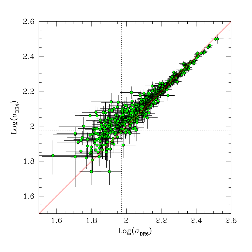
Figure 2: Comparison between Log($\sigma_{DR6}$) and Log($\sigma_{DR4}$) for 523 SDSS galaxies originally selected in the fields of our WINGS survey. Note the systematic offset between the DR4 and DR6 releases at low velocity dispersions.

It is worth pointing out that in the originally submitted version of this paper (arXiv0804.1892D) we used SDSS velocity dispersion data from a previous release of the survey (SDSS–DR4) and that the differences between the velocity dispersions given in DR4 and DR6 are not negligible, especially for small values of $\sigma$ (see Figure 2). This is the reason why many figures and tables, as well as some findings we report here (mainly concerning the difference between the FP coefficients of the SDSS and NFPS samples) are slightly different from the corresponding ones reported in the previous version of the paper. Still, we decided to keep that version unchanged on the babbage (just slightly modifying the title) in order to show how much a correct determination of the physical quantities involved in the FP (especially $\sigma$) is critical in drawing any conclusion from the FP tool.

All the available velocity dispersions have been homogenized to the uniform aperture $R_{e}/8$, following the recipe of Jørgensen et al. (1995). The estimated uncertainty for both surveys is in the range $7\div 10$%.

In Figure 3 we plot the difference Log($\sigma_{N}$)–Log($\sigma_{S}$) versus Log($\sigma_{N}$) for the $100$ galaxies of our sample in common between the NFPS and SDSS samples. The $rms$ scatter of the Log($\sigma_{N}$) vs Log($\sigma_{S}$) relation is $\sim 0.05$, equivalent to an uncertainty of $\sim 12$% in the common velocity dispersions. Again there is a systematic deviation between the two datasets at low velocity dispersions ($\sigma<95\ km\ s^{-1}$).

In the following, to avoid any possible bias in the comparison of the FP of clusters, we have excluded from our analysis the objects with $\sigma<95\ km\ s^{-1}$. Moreover, when dealing with the global (W+N+S) galaxy sample, the average velocity dispersion $\sigma=(\sigma_{N}+\sigma_{S})/2$ have been assigned to the galaxies in common between NFPS and SDSS.

Figure 3: The difference Log($\sigma_{S}$)–Log($\sigma_{N}$) versus Log($\sigma_{S}$) for the 100 ETGs of our sample in common between the NFPS and SDSS surveys. Note the systematic offset at low velocity dispersions, which led us to restrict our sample to galaxies with $\sigma>95\ km\ s^{-1}$.

3 FITTING THE FP

It is well known that the values of the FP coefficients vary systematically at varying the adopted fitting algorithm (Strauss & Willick, 1995; Blakeslee et al., 2002) and that the choice of the algorithm actually depends on the particular issue under investigation (relation among the physical quantities, linear regression for distance determination, etc..). Here we tried two different algorithms to get the best fit of the FP: 1) the program MIST, kindly provided by La Barbera et al. (2000), which is a bisector least square fit, coupled with a bootstrap analysis providing a statistical estimate of the errors of the FP coefficients; 2) a standard $\chi^{2}$ fit minimizing the weighted sum of the orthogonal distances (ORTH hereafter). Both algorithms account, in different ways, for the measurement errors on the variables Log($R_{e}$), $\langle\mu\rangle_{\rm e}$, and Log($\sigma$). MIST considers an average covariance matrix that includes the variances of the errors in all parameters and their mutual correlations (such as $rms_{Log(R_{e})}$ vs. $rms_{\mbox{$\langle\mu\rangle_{\rm e}$}}$). On the other hand, ORTH takes into account the errors of individual measures in a standard $\chi^{2}$ analysis. In Table 2 we report the FP coefficients derived from the two fitting algorithms for the global galaxy sample (first two lines) and for the NFPS and SDSS samples separately (lines 3-4 and 5-6, respectively). In the same table (lines 8-9) we report for comparison the FP coefficients obtained with both MIST and ORTH fitting algorithms for a sample of 80 ETGs in the Coma cluster (photometric and kinematical data from Jørgensen et al., 1995[JORG]). The column labeled with $N_{g}$ in the table reports the number of galaxies used in each fit.

Besides the best fitting algorithm, the FP coefficients might also be systematically influenced by the technique adopted to measure the effective radius and surface brightness of galaxies (1D/2D light profile fitting with de Vaucouleurs/Sersic laws). Lines 5 and 7 of Table 2 report the MIST FP coefficients obtained for the galaxy sample in common between WINGS and SDSS, using alternatively the two surface photometry data sets (see in Figure 1 the comparison among them and in Section 2.1 the description of the WINGS and SDSS surface photometry techniques). It is evident that, at least in our case, the influence of the adopted surface photometry technique on the FP coefficients turns out to be negligible.

Table 2 shows that different fitting algorithms (and, possibly, surface photometry techniques) lead to somewhat systematic differences in the FP coefficients. In particular, the values of $a$ obtained using the MIST fit are in general slightly smaller than those coming from the orthogonal fit. This means that, in order to perform a correct comparison of the FP results, it is advisable to adopt homogeneous FP fitting and (perhaps) surface photometry techniques.

However, in the present analysis, we do not focus on the ’true’ values of the FP coefficients. Instead, we will concentrate on their possible variation as a function of both galaxy and cluster properties. In other words, rather than in obtaining the best possible fit for a given application of the FP, we are interested in investigating the FP systematics, once both the fitting algorithm and the surface photometry technique have been chosen. Hereafter we adopt the MIST bisector fitting algorithm and the WINGS-GASPHOT surface photometry. The last choice will allow us to account for the structural non-homology of galaxies (Sersic index, see Section 6), while the former one will provide FP coefficients useful for distance determination of farther clusters. However, using the ORTH fitting algorithm, we will also provide in Section 5.3 a recipe for the V-band FP, useful to define the physical relation among the quantities involved in it.

Comparing each one another the FP coefficients given in Table 2, we easily realize that, besides the obvious dependence on the fitting algorithms, a further dependence exists on the galaxy sample, even adopting the same fitting algorithm (MIST) and surface photometry technique (WINGS-GASPHOT). In particular, the $a$ coefficient, which is related to the so called ’tilt’ of the FP, is noticeably different for the three data samples, even if the $rms$ scatter in Log($R_{e}$) is always $\sim 0.05$ (which implies an uncertainty of $\sim 12\%$), a value just a bit larger than that reported in Jørgensen et al. (1995) ($\sim 11\%$).

In panel (a) of Figure 4 we show the MIST bisector fit of the FP obtained for the whole W+N+S dataset (see line 1 of Table 2) using two different colors for the W+N and W+S data samples (respectively black and grey; green in the electronic form). Note the cut shown by SDSS data at large values of Log($R_{e}$), which is obviously due to the bright end cut of the survey.

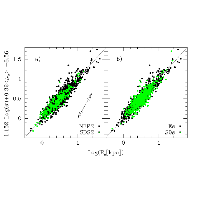
Figure 4: (panel a): The FP of the W+N (black dots) and W+S (gray dots; green in the electronic version) data samples; (panel b) The W+N+S FP for E (black dots) and S0 (gray dots; green in the electronic version) galaxies. In both panels we used for reference the FP coefficients derived from the best fit of the global dataset (W+N+S). The two-sided arrow in panel (a) roughly defines, through the Faber-Jackson (L$-\sigma$) relation, the direction of constant luminosity (or $\sigma$; see Section 4.2).

In Figure 5 we plot the FP of the individual clusters, again using for reference the coefficients derived from the fit of the whole W+N+S data sample. Columns 3-8 of Table 3 report the best fit coefficients (and the associated uncertainties) of each cluster, obtained with the MIST algorithm. Even from a quick look of both Figure 5 and Table 3, it is clear that the global fit does not seem to be a valid solution for all clusters.

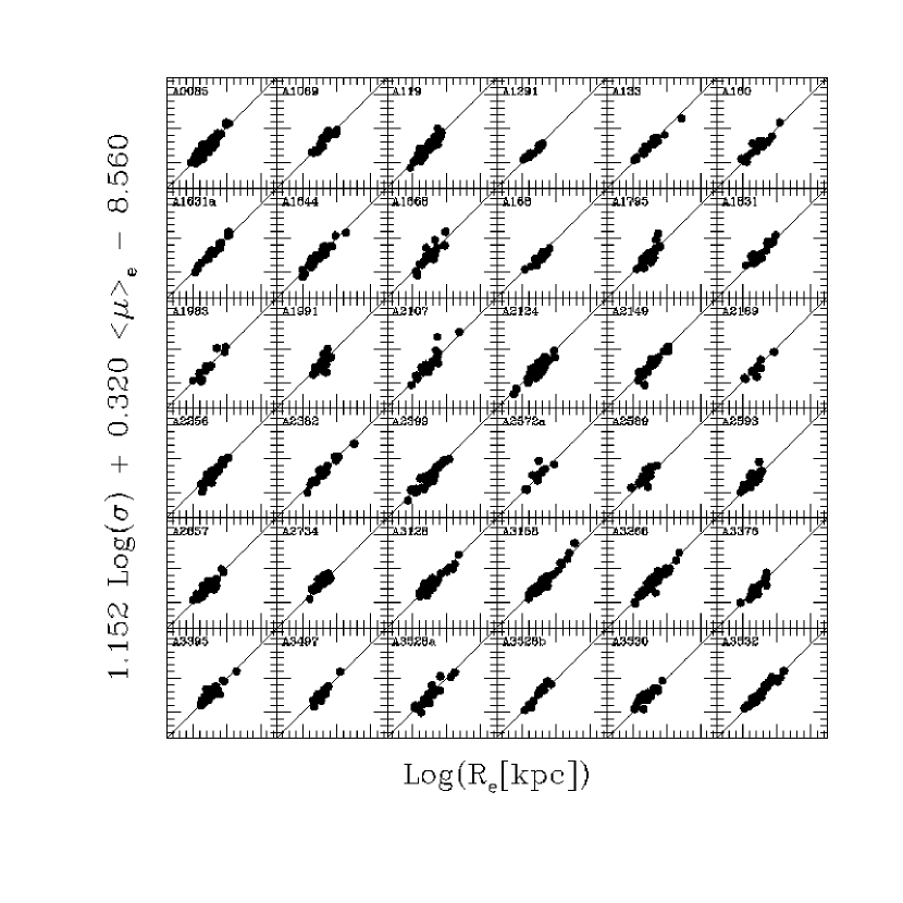
Figure 5: The FPs of individual clusters in our sample are plotted using the MIST best fit solution found for the global W+N+S galaxy sample.

Figure 5: The FPs of individual clusters (continued).

The average values (with their uncertainties), the standard deviations and the median values of the (MIST) FP coefficients of the clusters in the global sample and in the samples W+N and W+S are reported in Table. 4. From this table we note that: (i) even if the scatter is large, the average values of the FP coefficients appear systematically different (well beyond the expected uncertainties) in the W+N and W+S cluster samples, confirming the dichotomy already noted in Table 2; (ii) when just clusters with $N_{g}>N_{med}(=23)$ are considered, the standard deviations of the distributions of the FP coefficients decrease only slightly, suggesting that the large scatter cannot be ascribed to the statistical uncertainties related to the (sometimes) small number of ETGs in our clusters.

4 ORIGIN OF THE SCATTER OF THE FP COEFFICIENTS

We test two different hypotheses to explain the differences between the W+N and W+S samples and, in general, the large observed scatters of the FP coefficients: (i) they are simply due to the statistical uncertainties of the fits; (ii) they are artificially produced by the different criteria used to select ETGs in the NFPS and SDSS surveys.

4.1 Consistency with statistical uncertainties

First we test the ’null hypothesis’ that the observed scatter is merely consistent with the statistical uncertainties of the fits. To this aim, using all the galaxies in our sample, we produced two different sets of simulated clusters. In the first set we generate mock clusters with number of galaxies ($N_{g}$) progressively increasing from Log($N_{g}$) = 1 to 2 (step 0.1) and fit each mock cluster with MIST. Figure 6 shows the average values of the FP coefficients and the corresponding standard deviations as a function of Log($N_{g}$). Note that, since for each value of $N_{g}$ the whole sample of 1550 galaxies is used to randomly extract as many mock clusters as possible avoiding galaxy repetitions, the number of mock clusters increases at decreasing $N_{g}$, thus resulting in almost constant error bars of the average FP coefficients and of their variances.

Figure 6: Average values (left panels) and standard deviations (right panels) of the FP coefficients as a function of the number of galaxies ($N_{g}$) for mock clusters randomly extracted from the whole galaxy sample (see text for details). The dashed lines in the left panels correspond to the FP coefficients obtained fitting altogether with MIST the 1550 galaxies in our sample. The full lines in the right panels correspond to the simple exponential functions we used to compute the standard deviations as a function of Log($N_{g}$) (see the equations in each panel).

In the second set of simulations we produced 100 toy surveys, each containing 59 clusters obtained by sorting randomly the whole galaxy sample and taking sequentially the same number of galaxies per cluster as the real survey (thus avoiding galaxy repetitions). Then, using the MIST algorithm, we evaluate the FP coefficients of each mock cluster and, for each mock survey, we compute the average and median values of the coefficients, together with their standard deviations. Finally, we compare the distributions of the average coefficients and their variances in the mock surveys with the corresponding values of the real survey.

Figures 7 and 8 illustrate the conclusions of the two sets of simulations. The first set has been used to compute (with the equations given in the right panels of Figure 6) the error bars in Figure 7. The left panels of this figure report the FP coefficients of our ’real’ clusters versus the number of galaxies in each cluster, while the histograms on the right side of each panel show the corresponding distributions (see figure caption for more details). The error bars are used to compute the reduced Chi-square values (reported in the figure; in our case $\nu$=58) of the differences between the coefficients of the individual clusters and the corresponding coefficient of the global galaxy sample (dashed lines in the figure). Apart from the $a$ coefficient ($P_{\nu}\sim$0.965), they correspond to very high values of the rejection probability ($P_{\nu}>$0.995) that the coefficients of the individual clusters are randomly extracted from the same parent population.

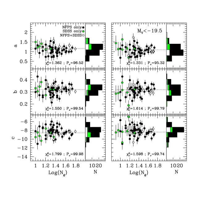
Figure 7: (Left panels): FP coefficients of our clusters versus the number of galaxies in each cluster. The black and gray (green in the electronic version) dots refer to clusters with only NFPS and SDSS galaxies, respectively. The open dots represent the seven clusters in common between the NFPS and SDSS surveys. The dashed lines correspond to the FP coefficients obtained fitting altogether with MIST the 1550 galaxies in our sample. The histograms on the right represent the distributions of FP coefficients in our cluster samples. Black, gray (green in the electronic version) and open histograms have the same meanings as in the left plots and are cumulated inside each bin; (Right panels): as in the left panels, but using only galaxies with $M_{V}<-19.5$. Note that in the left panels (global galaxy sample) the NFPS and SDSS clusters have quite different distributions of the coefficients, while in the right panels (just galaxies with $M_{V}<-19.5$) the distributions of the two samples are consistent among each other.

Figure 8 shows that the average values of the FP coefficients for the clusters of the real survey are just marginally consistent with the corresponding distributions obtained with the simulations of mock surveys (upper panels), while the distributions of variances are more or less in agreement with the real ones (lower panels).

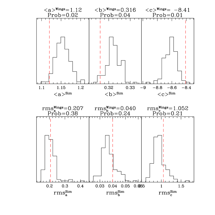
Figure 8: Histograms of the average values of the FP coefficients (upper panels) and standard deviations (lower panels) for the 100 toy surveys (see text for details). The dashed lines in the histograms mark the corresponding values obtained from the real survey (see Table. 4). These values are also reported in the panels, together with the probabilities that they are randomly extracted from the underlying histograms. Note in the upper panels that the average values of the FP coefficients for the clusters of the real survey are just marginally consistent with the corresponding distributions obtained from the mock surveys.

The two sets of simulations indicate that the observed scatter is not accounted for by the statistical uncertainties of the fits and that the real clusters cannot be merely assembled by random extraction of galaxies from the global population. The left panels of Figure 7 also clearly illustrate the systematic differences between the FP coefficients of the NFPS and SDSS samples already quoted in Tables 2 and 4. To this concern, the two–sample Kolmogorov–Smirnov test, applied to the black and open+gray(green) samples in that Figure, provides rejection probabilities of 0.998, 0.530 and 0.986 for the left panels coefficients $a$, $b$ and $c$, respectively.

4.2 Dependence on galaxy sampling

As an early test, we wanted to investigate the hypothesis that the observed scatter of differences in the FP coefficients are the result of blending E and S0 galaxies, with the knowledge that the E/S0 ratio varies (for example) as a function of local density. We verified that the FP computed separately for the elliptical and S0 galaxies are practically indistinguishable (all FP coefficients differ by $<3\%$; see also the right panels of Figure 4). This allows us to rule out the hypothesis that the observed scatter is induced by different E/S0 fractions in the different samples.

On the other hand, we have seen in Tables 2 and 4 that the FP coefficients of the clusters in the W+N and W+S data samples are systematically different from each other (see also the left panels of Figure 7 and the last sentence of the previous sub–section). It is therefore natural asking which is the origin of such systematic difference.

Since for all galaxies in the sample the surface photometry data come from WINGS+GASPHOT, we could be tempted to conclude that the differences we found are due to some systematic offset between velocity dispersion measurements from the NFPS and SDSS surveys. However, this possibility is definitely ruled out by Figure 3 (Sec. 2.2), which shows that the agreement between the two velocity dispersion surveys is fairly good, at least for $\sigma>$95km s^-1. Indeed, we have also verified that the FP coefficients of the galaxy sample in common between NFPS and SDSS, obtained using alternatively the two velocity dispersion data sets do not differ significantly.

Thus, we are left with the last possibility: that the systematic FP differences between the NFPS and SDSS clusters are due to the different distributions of photometric/kinematic properties of galaxies in the two samples. The danger of selection biases in this game has already been emphasized by Lynden-Bell et al. (1988), Scodeggio et al. (1998), and Bernardi et al. (2003), who showed that robust fits of the FP can be obtained only for galaxy samples complete in luminosity, volume, cluster area coverage and stellar kinematics. The panels (a) and (b) of Figure 9 respectively show the projection of the FP on the surface photometry plane ($\langle\mu\rangle_{\rm e}-{\rm Log}(R_{\rm e})$ ; Kormendy relation) and the Color-Magnitude diagrams [$M_{V}-(B-V)$] for the NFPS and SDSS surveys. Both figures show that the two galaxy samples have quite different distributions of the photometric quantities involved in the FP parameters. This is even more evident in the panel (c) of the same figure, where the face-on view of the FP of the global sample is shown, together with the loci corresponding to some constant values of the quantities involved in the FP (dotted lines). Note that, both in the Color-Magnitude and in the Kormendy diagrams, the W+S galaxy sample turns out to be (on average) fainter than the W+N sample, especially in the small size region. This is likely a direct consequence of the rules the two surveys adopt to select early-type galaxies (see Section 2.2).

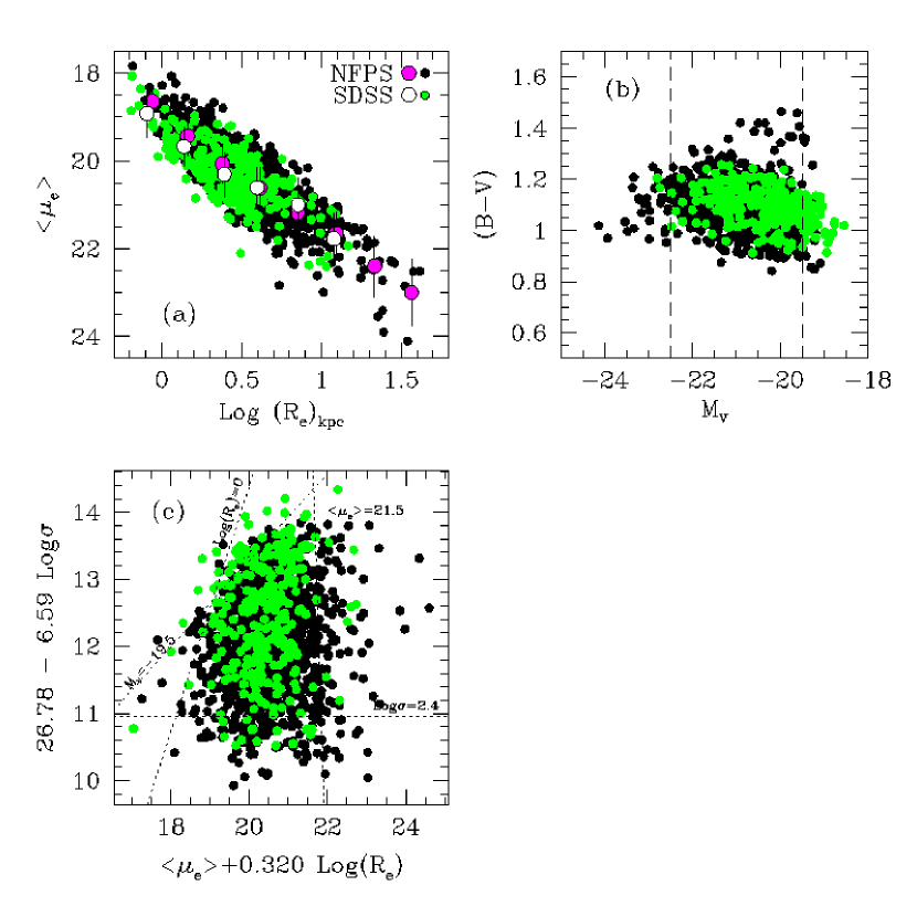
Figure 9: (Panel a): the $\langle\mu\rangle_{\rm e}-{\rm Log}(R_{\rm e})$ relation for the W+N (black dots) and W+S (gray dots; green in the electronic version) samples. The big dark-gray (magenta in the electronic version) and white dots represent the average surface brightnesses of the two galaxy samples in different bins of Log($R_{e}$); (Panel b): the Color-Magnitude diagrams for the galaxies of the W+N and W+S samples. Symbols are as in panel (a); (Panel c): face-on view of the FP obtained for the global galaxy sample. The dotted straight lines mark the loci corresponding to some constant values of luminosity, surface brightness, effective radius and velocity dispersion. Symbols as in the previous panels.

The fact that such differences in the galaxy sampling produce the observed differences in the FP coefficients is shown in Figure 10. In the upper panels of the figure the $a$ coefficient of the FP seems to be anti-correlated with the average values of luminosity, radius and velocity dispersions of galaxies in the clusters. The same, but (obviously) with positive CCs, happens for the coefficient $c$ (not reported in the figure). We see from the lower panels in the figure that, if we cut the data samples at higher luminosity, $M_{V}=-19.5$, these correlations disappear, since in this case the two data samples are more homogenous.

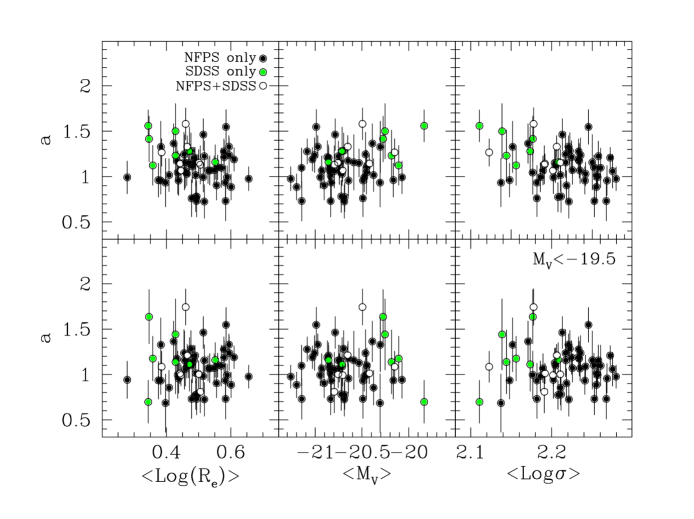
Figure 10: (Upper panels) the FP coefficient $a$ vs. the average values of effective radius ($<Log(\mbox{$R_{\rm e}$})>$), luminosity ($<M_{V}>$) and central velocity dispersion ($<Log(\sigma)>$) of the galaxies in each cluster. Symbols are as in Figure 7. (Lower panels) the same plots, but using only galaxies with $M_{V}<-19.5$.

This is also confirmed by the right panels of Figure 7, where the plots in the left panels are repeated using only galaxies with absolute magnitude $M_{V}<-19.5$. Indeed, the two–sample Kolmogorov–Smirnov test, applied to the black and open+gray(green) samples in that figure, provides rejection probabilities of 0.475, 0.308 and 0.318 for the right panels coefficients $a$, $b$ and $c$, respectively (compare these values with those given in the last sentence of Section 4.1)

A final, quantitative estimate of the dependence of the FP coefficients on the luminosity distribution of the galaxy sample is provided by Figure 11, where we report the FP coefficients obtained for different values of the faint and bright luminosity cut-off applied to the NFPS and SDSS samples.

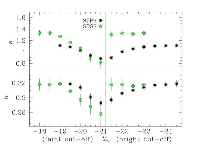
Figure 11: The FP coefficients $a$ and $b$ obtained with MIST for different values of the faint and bright luminosity cut-off applied to the NFPS galaxy sample (black dots) and to the SDSS sample (gray dots; green in the electronic version).

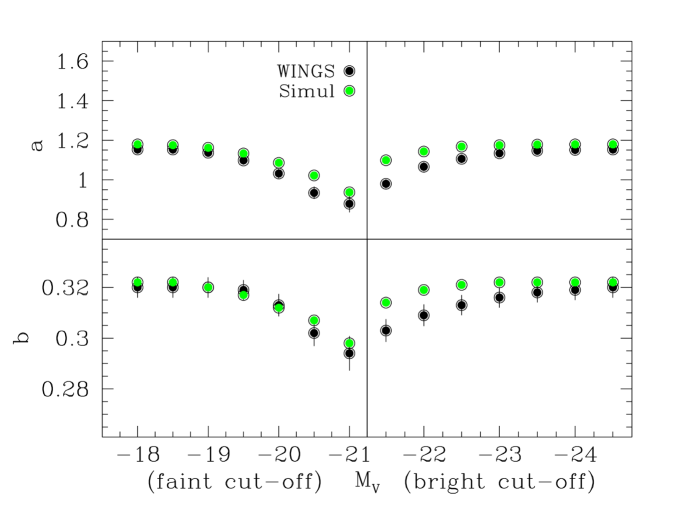
Figure 12: similar to Figure 11, but comparing the W+N+S sample (black dots) with a mock sample of 10,000 toy galaxies (grey dots; green in the electronic version of the paper; see text for more datails)

The left panels of Figure 11 show that, for both the NFPS and the SDSS sample, the coefficients $a$ and $b$ decrease at increasing the faint luminosity cut. This effect can be at least partially explained by the very geometry of the FP. In fact, in the edge-on representation of the FP, any luminosity cut in the galaxy sample translates, through the Faber-Jackson (L$-\sigma$) relation, in a sort of ’zone of avoidance’ delimited by a line of constant luminosity (or $\sigma$), whose direction is roughly indicated by the two-sided arrow in Figure 4 (panel a). This Malmquist-like bias reduces the FP slopes along the directions of $\sigma$ and $\langle\mu\rangle_{\rm e}$ for both faint- and bright-end luminosity cuts. Figure 12 illustrates this ’geometrical’ effect. It is similar to Figure 11, but compares the W+N+S sample (black dots) with a mock sample of 10,000 toy galaxies (grey dots; green in the electronic version of the paper) randomly generated around the same (W+N+S) FP, according to the ’true’ distributions (and mutual correlations) of $\langle\mu\rangle_{\rm e}$  $R_{\rm e}$ and $\sigma$. The right panels of Figure 11 show that this bias actually works for the bright-end luminosity cut just in the case of the NFPS sample. Instead, the FP coefficients of the SDSS sample display a rather peculiar behaviour. For the faint-end cuts they show trends similar to those of the NFPS sample, but more pronounced. Instead, they do not seem to depend at all on the bright-end cuts (right panels), remaining significantly higher than in the case of the NFPS samples over the range of cut-off luminosities. This behaviour suggests that, besides the luminosity cut-off, other causes may contribute to tell apart the two samples.

Figure 13: Edge-on FP as it appears along the direction of luminosity. Symbols are as in panel (a) of Figure 4. The black curve (red in the electronic version) just represents a naive fitting we made in order to enhance the warp-like feature of this particular projection of the FP.

The Figure 13 helps to clarify this point. It shows the edge-on FP as it appears along the direction of luminosity. This particular projection highlights a weak feature of the FP that otherwise would be completely masked, suggesting the existence of a sort of warping (black curve in the figure; red in the electronic version). Although just hinted in the bright part of the luminosity function, this feature looks a bit more evident in its faint-end, which in our sample is dominated by SDSS galaxies. To this concern, it is worth noticing that this faint luminosity warp can hardly be attributed to a possible upward bias of the SDSS low velocity dispersion measurements, since, according to Smith et al. (2004) (see also Figure 3), such a bias should in case work in the opposite direction. The different shape of the NFPS and SDSS samples in this particular projection of the FP explain the reasons why: (i) for the SDSS sample the coefficient $a$ turns out to be always greater than in the case of the NFPS sample; (ii) the faint-end luminosity cut influences the coefficient $a$ of the FP more for the SDSS than for the NFPS sample; (iii) the bright-end luminosity cut does not influence the FP coefficients of the SDSS sample.

Although these analyses would benefit from a more robust statistic, they lead us to suggest that the FP is likely a curved surface. This fact has been recently claimed by Desroches et al. (2001) and, in the low-luminosity region, may actually indicate a first hint of the connection between the FP of giant and dwarf ellipticals (Nieto et al., 1990, Held et al., 2001, Peterson and Caldwell, 1993). In Section 6 we will also present a further hint of the existence of the high luminosity warp of the FP suggested by Figure 13.

It is important to stress that the possible curvature of the FP may give rise to different values of its coefficients when different selection criteria, either chosen or induced by observations, are acting to define galaxy samples. This fact represents a potentially serious problem when the goal is to compare the tilt of the FP at low- and high-redshifts, since it implies that a reliable comparison can be done only if galaxy samples at quite different distances share the same distributions of the photometric/kinematic properties, which is indeed not usually the case.

Finally, we note that, according to the Chi-square values reported in the right panels of Figure 7, the scatter of the FP coefficients is poorly consistent with the expected statistical uncertainties, even after having reduced the annoying dichotomy between the NFPS and SDSS data samples. This fact suggests that at least part of the observed scatter must be somehow ’intrinsic’ and resulting from a ’true’ dependence of the FP coefficients on the galaxy properties and/or on the local environment and/or on the global cluster properties. The huge amount of data available from the WINGS photometric catalogs allows us to perform for the first time this kind of analysis.

5 SYSTEMATICS OF THE FP COEFFICIENTS

In order to reduce the luminosity-driven bias of the FP coefficients illustrated in the previous Section 4.2, we decided to use in this section only galaxies with $M_{V}<-19.5$ ($N_{g}$=1477). Even if this luminosity cut-off does not remove completely the systematic FP differences arising from the different sampling rules of the NFPS and SDSS surveys (see Figure 11), we guess it is able at least to reduce them down to an acceptable level.

5.1 FP versus galaxy properties and local environment

In Section 4.2 we have already shown that the FP coefficients do depend on the average luminosity of the galaxies in the sample and, therefore, on the average values of size and velocity dispersion (see Figure 10). These dependences concern the very shape of the FP relation, since they involve the physical quantities defining the relation itself. Now, besides these ’first order’ dependences, we want to check whether the FP relation varies with other galaxy properties or the local environment. In particular, as far as the galaxy properties are concerned, we test the ($B-V$) color, the Sersic index Log($n$) and the axial ratio $b/a$, while the cluster-centric distance $D_{CC}$ (normalized to $R_{200}$ ) and the local density Log($\rho$) are used as test quantities of the local environment.

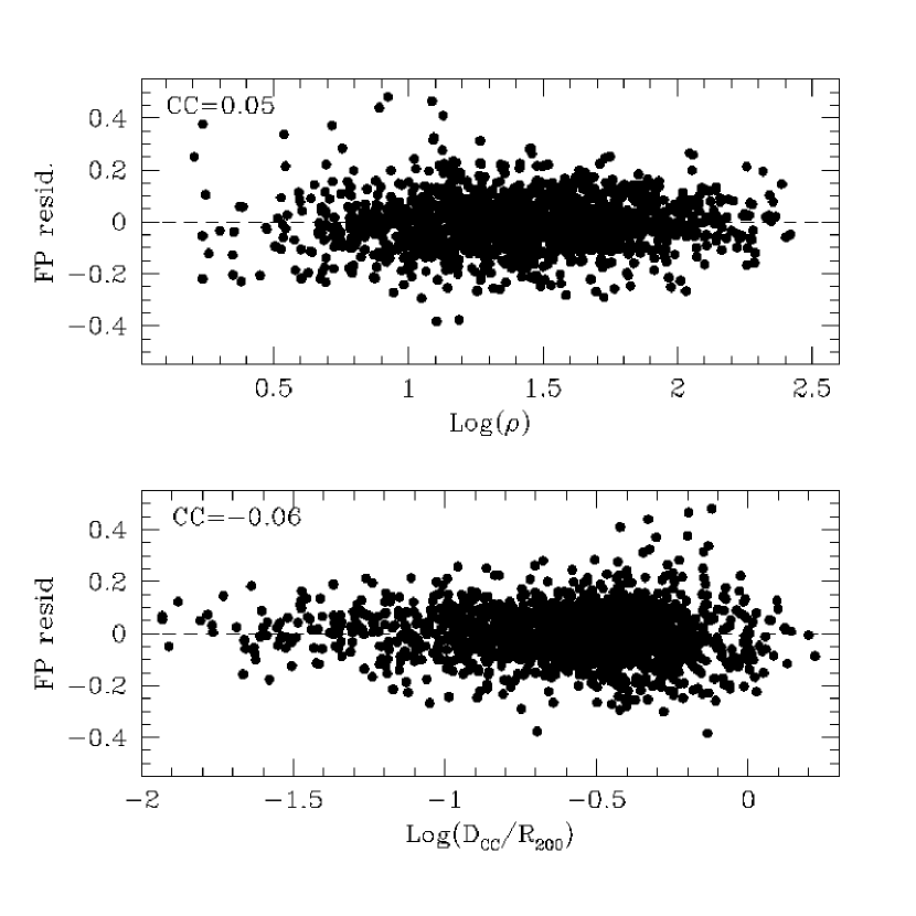
Figure 14: The residuals of the FP fit versus the local density (upper panel) and the normalized cluster-centric distance (bottom panel). Note the lack of correlation in this plots with respect to that found in Figure 15.

A simple way to perform such kind of analysis is to correlate the test quantities with the residuals of the FP relation obtained for the global galaxy sample (Jørgensen et al., 1996). For instance, in Figure 14 the FP residuals are reported as a function of both $D_{CC}$ and Log($\rho$). From this figure one would be led to conclude that these two parameters do not influence at all the FP coefficients. However, this method would be intrinsically unable to detect any correlation if the barycentre of galaxies in the FP parameter space does not change at varying the test quantity. In fact, in this case, any change of the slope alone would produce a symmetric distribution of the positive and negative residuals, keeping zero their average value. For this reason, we preferred to perform the analysis by evaluating the FP of galaxies in different bins of the test quantities. Moreover, in order to get similar uncertainties of the FP coefficients in the different bins, we decided to set free the bin sizes, fixing the number of galaxies in each bin ($N_{bin}$).

In Figure 15 the average values of the the FP coefficients in different bins of the test quantities are plotted as a function of the median values of the quantities themselves inside the bins. The panels also report the correlation coefficients ($CC$) of the different pairs of bin-averaged quantities. In these plots we set $N_{bin}$=150 and assumed the centers of the clusters to coincide with the position of the BCGs. However, the trends and the correlation coefficients in the figure remain almost unchanged if we set (for instance) $N_{bin}$=200 and assume that the cluster centers coincide with the maximum of the X-Ray emission.

It is worth stressing that the FPs we obtain with the outlined procedure for each bin of the test quantities do not refer to real clusters. They are actually relative to ideal samples for which some galaxy/environment property is almost constant (for instance: constant local density).

Figure 15: Average values of the the FP coefficients in different bins of color [($B-V$)], Sersic index [Log($n$)], axial ratio [$b/a$], clustercentric distance [Log($D_{CC}/R_{200}$)] and local density [Log($\rho$)] as a function of the median values of the same quantities inside the bins. The number of galaxies per bin is fixed to 150 and the BCGs are assumed to coincide with the centers of the clusters. The correlation coefficients of the different pairs of bin-averaged quantities are also reported in the panels. Note the strong correlations between the FP coefficients and the environment parameters $D_{CC}$ and $\rho$.

At variance with the conclusions one could draw from Figure 14, it is clearly show in Figure 15 that strong correlations exist between the FP coefficients and the environment parameters ($D_{CC}$ and $\rho$), while the correlations are less marked (or absent) with the galaxy properties. We have verified that the average (and median) absolute magnitudes do not vary significantly in the different bins of the test quantities Log($D_{CC}$) and Log($\rho$). Thus, the correlations among these quantities and the FP coefficients cannot be induced by the above mentioned dependence of the FP coefficients on the absolute magnitude (see Sec. 4.2). Moreover, the lack of correlation in the three uppermost panels of Figure 16 rules out the possibility that the above trends just reflect similar trends involving the very physical quantities that define the FP.

Figure 15 suggests that, in the FP, the dependences on both velocity dispersion and average surface brightness of galaxies become lower and lower as the distance from the cluster center increases. Looking at the two leftmost panels of Figure 15, one could wonder if the further dependences of the FP coefficients on both the Sersic index (stronger) and the color (weaker) are merely reflecting the correlation with the clustercentric distance. The lack of correlation in the two lowest panels of Figure 16 help to clarify this point, suggesting that light concentration and color could actually be additional (independent) physical ingredients of the FP recipe. It is also interesting to note in Figure 15 that the $b$ coefficient correlates quite well with the Sersic index $n$, while $a$ does not. This is likely because $b$ is the coefficient associated with the photometric parameter $\langle\mu\rangle_{\rm e}$ , which is in turn obviously related to the concentration index $n$. Finally, we note that, from the very (linear) expression of the FP, most of the dependences of the $c$ coefficient on the various test quantities in Figure 15 are likely induced by the corresponding dependences of the $a$ and $b$ coefficients, any increase of the last ones producing necessarily a decrease of the former one, and viceversa.

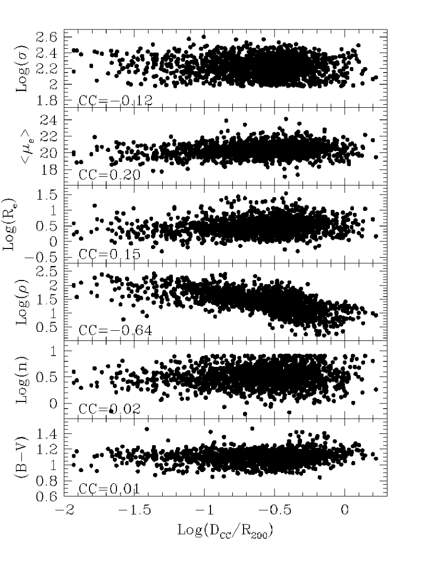
Figure 16: Normalized cluster-centric distance versus velocity dispersions, effective surface brightness, effective radii, local density, Sersic index and color for our sample of early-type galaxies with $M_{V}<-19.5$. Note the well known (obvious) dependence of the local density on the clustercentric distance, while the other panels display the substantial lack of correlations with the other variables. The obvious cut at large $Log(n)$ is due to the intrinsic limit of GASPHOT to give Sersic index $n>8$.

The trends observed in Figure 15 further confirm that the FP coefficients depend on the particular criteria used in selecting the galaxy sample. They are also likely able to explain the large scatter of the FP coefficients which is found even after removal of the luminosity-driven bias discussed in Section 4.2 (high values of $\chi^{2}_{\nu}$ and $P_{\nu}$ in Figure 7).

5.2 FP versus global cluster properties

We have also explored the possible dependence of the FP coefficients (in particular of the coefficient $a$) on several measured quantities related to the global cluster properties. Tentative correlations have been performed with the velocity dispersion of the galaxies in the clusters, with the X-Ray luminosity, with redshift, with the integrated V-band luminosity (within $M_{V}=-19.5$) of the clusters, with different kinds of cluster radii, with the average Sersic index of the cluster galaxies, with the average Log($M/L$), etc. Some of these plots are shown in Figure 17. No significant correlations have been found.

Figure 17: From top to bottom: the FP coefficient $a$ versus the number of galaxies (with $M_{V}<-19.5$) in the cluster, the radius of the cluster $R_{200}$, the X-ray luminosity, the $rms$ of peculiar velocities of galaxies in the cluster, the integrated V-band luminosity (again with $M_{V}<-19.5$) and the redshift. No significant correlations are found.

5.3 Can we provide a general recipe for deriving the FP ?

From the analysis performed in Section 4, the differences in the FP coefficients appear to be related to sampling aspects (i.e. the luminosity cut-off). In Section 5 we have shown that, although not depending on the global cluster properties, the FP coefficients are also strongly related to the environmental properties of galaxies ($D_{CC}$ and $\rho$) and to their internal structure (Sersic index). These dependences likely concern the very formation history of galaxies and clusters. They are not strictly referable as sampling effects, but we can of course always speak of sampling, as far as they translate into the photometric properties of galaxies. This let us understand that the various dependences are actually linked each other and it is not easy to isolate each of them. Moreover, it is worth stressing that the previous analyses (never tried before) have been made possible just because we have at our disposal a huge sample of galaxies, obtained putting altogether data from many different clusters. When dealing with the determination of the FP for individual (possibly far) clusters, we usually must settle for what we actually have, that are a few galaxies (a few dozens, in the most favourable cases) with different luminosities and structures, located in a great variety of environments. In this cases, we can hardly renounce to each single galaxy and the above dependences turn out to be irreparably entangled each one another.

From the previous remarks it stands to reason that, even with our large sample of galaxies, to provide a general recipe for determining unbiased coefficients of the FP in individual clusters is far from being a realistic objective. The best we can do is to remove from our global (W+N+S) sample the low-luminosity galaxies ($M_{V}>$-19.5; see Section 4.2) and to provide, for this restricted sample, the FP coefficients obtained with both MIST and ORTH fitting algorithms. They are:

$a=1.097\pm 0.020;b=0.318\pm 0.004;c=-8.41\pm 0.097$ (MIST)

$a=1.208\pm 0.052;b=0.318\pm 0.010;c=-8.65\pm 0.19$, (ORTH)

which we assume to define the global (unbiased, as far as possible), V-band FP of early-type galaxies in nearby clusters. The MIST coefficients are more suitable for distance determination, while the ORTH ones more properly define the physical relation among the quantities involved in the FP.

Columns 10-15 of Table 3 report the FP coefficients of the individual clusters obtained running MIST just for galaxies with $M_{V}<$-19.5.

6 THE $M/L_{V}$ RATIO OF EARLY-TYPE GALAXIES IN NEARBY CLUSTERS

The variation of the mass-to-light ratio with luminosity is the most popular explanation for the tilt of the FP with respect to the virial expectation. Therefore, it is important to analyse the $M/L$ ratio of cluster galaxies with our extensive photometric data, which account for the non homologous structure of the ETGs by means of the Sersic parameter $n$.

According to di Serego et al. (2005) (see also Michard, 1980), we calculate the dynamical mass of galaxies using the formula: $M/M_{\odot}=K_{V}(n)\sigma^{2}R_{e}/G$, where the virial coefficient $K_{V}(n)$ is a decreasing function of the Sersic index $n$ (Bertin et al., 2002) and $G$ is the gravitational constant.

Figure 18 shows the mass-to-light ratio as a function of mass for our global galaxy sample. The full straight line in the figure represents the linear fit obtained minimizing the weighted sum of perperdicular distances from the line itself [see the equation F(M) in the figure]. The open dots refer to the sample of galaxies in Coma given by Jørgensen et al. (1996), with the relative orthogonal fit represented by the dashed line. Note in particular that in our global sample the scatter of the residuals relative to the best-fit relation is greater than in the Coma sample (0.19 vs. 0.11; for the NFPS and SDSS samples the scatters are 0.18 and 0.21, respectively). However, we recall that Jørgensen et al. (1996) derived the photometric parameters ($R_{\rm e}$ and $\langle\mu\rangle_{\rm e}$ ) and the mass by assuming $r^{1/4}$ luminosity profiles, while we adopted the more general Sersic profiles. This might also explain the fact that the slope of the relation for our global sample [0.511($\pm$0.019)] is much larger that in the Coma sample [0.28($\pm$0.028)]. By the way, the slopes we found for the NFPS and SDSS samples separately, are quite consistent each other, within the errors [0.522($\pm$0.022) and 0.600($\pm$0.052), respectively].

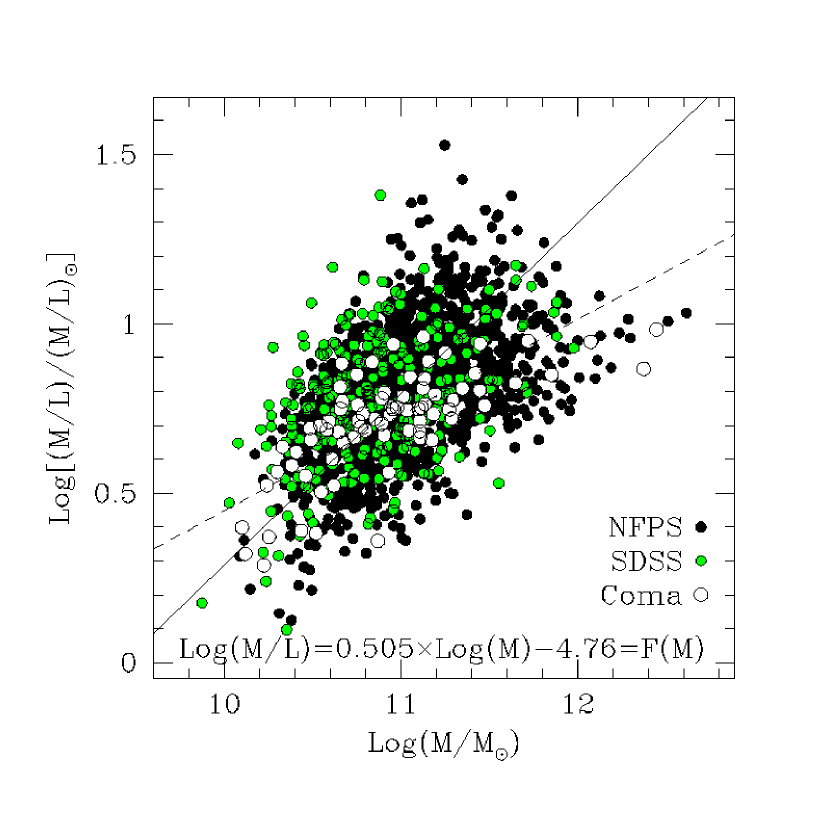
Figure 18: Mass-to-light ratio versus dynamical mass for our global galaxy sample. Black and gray (green in the electronic version) dots refer to W+N and W+S galaxies, respectively, while open dots refer to a sample of galaxies in Coma (see text). The solid line gives the orthogonal fit of the W+N+S data, while the dashed line reports the fit for the Coma sample.

Figure 19 reports several plots showing the correlations among different measured and evaluated quantities involving the mass-to-light ratio estimate. In particular we test (at the ordinate) dynamical masses, mass-to-light ratios and residuals [Log(M/L)-F(M)] of the relation in Figure 18 versus (at the abscissa) Sersic indices, velocity dispersions, effective radii and luminosities.

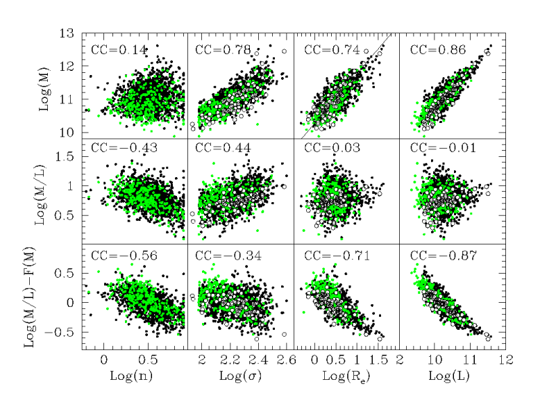
Figure 19: Correlations among measured (abscissa) and evaluated (ordinate) quantities involved in the mass-to-light ratio estimate. In each panel the proper correlation coefficient is also reported. Symbols are as in Figure 18. The straight line reported in the plot Log(M) - Log$R_{e}$ represents the orthogonal best-fit of the data we discuss in the last paragraph of this Section.

Some of the correlations in Figure 19 are well known (i.e. mass vs. luminosity), obvious (i.e. $M/L$ residuals vs. luminosity), or expected by definition (i.e. mass vs. $\sigma$ and $R_{\rm e}$ ). Less obvious seem to be some other correlations (i.e. $M/L$ vs. $\sigma$ and $M/L$ residuals vs. $\sigma$ and $R_{\rm e}$ ) or lack of correlations (i.e. $M$ vs. Sersic index, $M/L$ vs. $R_{\rm e}$ and luminosity). For instance, according to the formula we used to derive the dynamical mass, it should be a strongly decreasing function of the Sersic index (see Bertin et al., 2002), while the correlation coefficient of the plot $M$-$n$ in Figure 19 is slightly positive. Moreover, in the same figure the $M/L$ ratio does not seem to correlate at all with either radius or luminosity, while a correlation $M/L$-$L$ has been often claimed to explain the ’tilt’ of the FP.

In Figure 19 we find of particular interest the correlation between $M/L$ and Sersic index and that between $M/L$ residuals and Sersic index. The first one, coupled with the lack of correlation between $M/L$ and luminosity (which is indeed expected for non homologous ETGs, as suggested by Trujillo et al., 2004), indicates that, for a given luminosity, the galaxies showing lower light concentration (lower Sersic index) are more massive (more dark matter?).

The second, even stronger correlation is quite interesting as well. In fact, from the very definition of the $M/L$ residuals of the relation in Figure 18, for a given dynamical mass, the lower the residual, the brighter the galaxy. Therefore, the correlation in Figure 19 between $M/L$ residuals and Sersic indices implies that (again for a given mass) the higher the light concentration (Sersic index), the brighter the galaxy.

Thus, the picture emerging about the influence of the light concentration in determining dynamical mass and luminosity of ETGs is that: (i) for a given luminosity, the higher the light concentration, the lower the dynamical mass; (ii) for a given dynamical mass, the higher the light concentration, the higher the luminosity. This twofold dependence on the Sersic concentration index is expressed by the linear equation:

Log(n)=1.60$\times$Log(L)$-$1.16$\times$Log(M)$-$2.93,

we have derived minimizing the orthogonal distances from the fitting plane of the points in the parameter space ($n$,$L$,$M$). Note that the correlation coefficient between the Sersic index computed from this equation and the measured one is $CC$=0.59.

Still concerning the influence of the light concentration on the mass-to-light ratio of early-type galaxies, it is well known that the Sersic index $n$ correlates with the velocity dispersion (Graham, 2002). Thus, it is not meaningless wondering if the correlations involving $n$ in Figure 19 just reflect the correlations with $\sigma$. The upper and middle panels of the figure clearly rule out this hypothesis as far as the correlations with mass and mass-to-light ratio are concerned (both are positive for $\sigma$, while for $n$ they are close to zero and negative, respectively). Instead, the correlations of the $M/L$ residuals with $n$ and $\sigma$ (lower panels) have the same sign. It is worth noting, however, that the correlation turns out to be tighter with $n$ than with $\sigma$ and that the same happens (even if with opposite trends) also for the $M/L$ ratio in the middle panels of the figure. This might suggest that the driving parameter for $M/L$ is actually the light concentration and that the trends with $\sigma$ are just consequence of that.

We have previously guessed that the different slopes we find in the relation ($M/L$–$M$) between our sample and the Coma sample could be at least partially due to the different models of luminosity profiles used to derive the photometric parameters of galaxies (Sersic law and $r^{1/4}$ law, respectively). Now, we could legitimately guess that the correlations shown in the leftmost panels of Figure 19 are artificially produced by the use of the Sersic law in deriving the parameters $R_{e}$ and $K_{V}$, involved in the computation of the galaxy mass. Actually, $K_{V}$ turns out to be a decreasing function of the Sersic index (see Bertin et al., 2002), just like the $M/L$ ratio and the $M/L$ residuals in Figure 19 (but, in the same figure note the direct, although weak, correlation between the mass and the Sersic index!).

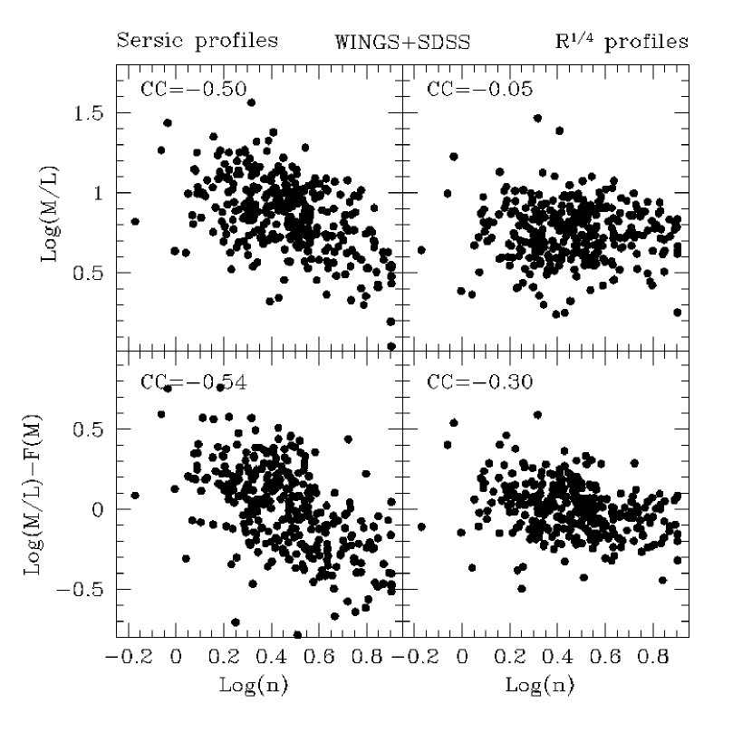
Figure 20: The $M/L$ ratio and the residuals of the $M/L$–$M$ relation versus the Sersic index for the W+S galaxy sample alone. Left and right panels illustrates the relations obtained using the Sersic and $R^{1/4}$ surface photometry parameters, respectively, in the computation of masses and luminosities. Again, the correlation coefficients are reported in each panel.

Trying to clarify these points, we have re-calculated the masses and the luminosities of the early-type galaxies in the original W+S sample (397 objects, before selection on $\sigma$ and $M_{V}$) using the surface photometry parameters provided by the SDSS database ($r^{1/4}$ profiles). In Figure 20 we plot the $M/L$ ratio and the residuals of the $M/L$–$M$ relation versus the Sersic index for the W+S galaxy sample alone. Left and right panels illustrate the relations obtained when masses and luminosities are computed using the Sersic and $r^{1/4}$ surface photometry parameters, respectively. In the former case, the correlation coefficients turn out to be undistinguishable from those obtained for the whole (W+N+S) galaxy sample (see Figure 19). In the latter case the correlations are less pronounced, but still they are in place, as indicated by 10,000 random extractions of couples of uncorrelated vectors having the same dimension (397) and distributions of the real ones. In fact, the probability that the correlation coefficients of the real sample in the right panels of Figure 20 are drawn from a parent population of uncorrelated quantities turns out to be very small: $\sim$0.005 and $\sim$0 for the correlations in the upper-right and lower-right panels, respectively. This enforces our previous conclusions about the dependence of masses and luminosities of early-type galaxies on the Sersic index. The weaker correlations found with the $r^{1/4}$ profiles if compared with the Sersic profiles, are likely the consequence of having forced the real luminosity structure of galaxies to obey the de Vaucouleurs law. Finally, we mention that the slope of the relation ($M/L$–$M$) for the W+S sample turns out to be 0.47 and 0.38 with the Sersic– and $r^{1/4}$–law approaches, respectively, thus confirming our previous guess that it is influenced by the assumption about the luminosity profile of galaxies (see the comparison between our sample and the Coma sample in Figure 18).

In a recent paper Robertson et al. (2006) claim that the tilt of the FP is closely linked to dissipation effects during galaxy formation. They show the results of their simulations in a plot of $M/M_{\odot}$ vs. the radius ($R$) of the galaxies. Figure 19 also shows a similar plot for our galaxy sample. Although a correlation between $M$ and $R_{e}$ is expected from the very definition of dynamical mass, we note in this plot that the more massive objects are preferably found below the orthogonal best-fit of the data distribution (by the way, these objects are those deviating in the high luminosity region from the FP projection in Figure 13). High luminosity objects also deviate with respect to the bulk of the early-type population in the $R-L$ relation, that for our global sample has the same slope found by Bernardi et al. (2007) ($R\propto L^{0.68}$). The systematically larger size of these galaxies in that relation may be consistent with the results of the simulations by Robertson et al. (2006), if one invokes the dry dissipationless merger mechanism for their formation. It again points towards the hypothesis that the FP relation might be non linear, this time in its high-mass region (see Section 4.2 for a similar finding in the low-mass region). Thus, in the parameter space of the FP the real surface defined by ETGs could be slightly bent, reflecting the different formation mechanisms producing the present day ETGs. In Section 4.2 we have seen that part of the scatter of the FP coefficients is just due to such an effect, coupled with the different statistical properties of the galaxy samples. As a consequence, to draw any conclusion about luminosity evolution and downsizing effect might be dangerous (the slopes of the relations depend on the sample selection rules/biases), unless the galaxy samples involved in these analyses, even spanning wide ranges of redshift, share the same distributions of photometric/kinematic properties of galaxies.

7 CONCLUSIONS

We have derived the Fundamental Plane of early-type galaxies in 59 nearby clusters ($0.04<z<0.07$) by exploiting the data coming from three big surveys: WINGS(W), to derive $R_{\rm e}$ and $\langle\mu\rangle_{\rm e}$ , and NFPS+SDSS(N+S), to derive $\sigma$. The fits of the FP, obtained for the global samples W+N and W+S, as well as for each cluster, have revealed that the FP coefficients span considerable intervals. By means of extensive simulations, we have demonstrated that this spread is just marginally consistent with the statistical noise due to the limited number of galaxies in each cluster. It seems at least partly due to a luminosity-driven bias depending on the statistical properties of the galaxy samples. These can be induced both by observing limitations and by selection rules. In fact, even if the best-fitting solution obtained for the global W+N+S dataset does not differ significantly from previous determinations in the literature, systematic different FP coefficients are found when the galaxy samples are truncated in the faint-end part at different cut-off absolute magnitudes. We speculate that, rather than a plane, the so called FP is actually a curved surface, which is approximated by different planes depending on the different regions of the FP space occupied by the galaxy samples under analysis. To this concern, we could go farther on in the speculation, suggesting that a bent FP could be, at least partially, reconciled with the numerical simulations in $\Lambda$CDM cosmology (see Borriello et al., 2003). By the way, such a speculation could also be supported by the large scatter we find in the $M/L$–$M$ relation, at variance with other determinations, whose tightness has been sometime invoked to rule out the hierarchical scenario.

Perhaps the most interesting result of the present analysis concerns the dependence of the FP coefficients on the local environment, which clearly emerges when we derive the FP in different bins of the cluster-centric distance and local density. Finally, we do not find any dependence of the FP coefficients on the global properties of clusters.

Concerning the $M/L$ ratio, we also find that both $M/L$ and the residuals of the $M/L$–$M$ relation turn out to be anti-correlated with the Sersic indices. These trends could imply that, for a given luminosity, more massive galaxies display a lower light concentration, while for a given dynamical mass, the higher the light concentration, the brighter the galaxy.

The main results of this work can be summarized as follows:

• the FP coefficients depend on the adopted fitting technique and (marginally) on the methods used to derive the photometric parameters $R_{\rm e}$ and $\langle\mu\rangle_{\rm e}$ ;

• The observed scatter in the FP coefficients cannot be entirely ascribed to the uncertainties due to the small number statistics;

• the FP coefficients depend on the distributions of photometric/kinematic properties of the galaxies in the samples (mainly on the faint-end luminosity cut-off);

• the FP coefficients are strongly correlated with the environment (cluster-centric distance and local density), while the correlations are less marked (or absent) with the galaxy properties (Sersic index, color and flattening);

• the FP coefficients do not correlate with the global properties of clusters (radius, velocity dispersion, X-ray emission, etc..);

• the distribution of galaxies in the FP parameter space suggest that the variables $R_{\rm e}$, $\langle\mu\rangle_{\rm e}$ , and $\sigma$ define a slightly warped surface. Forcing this surface to be locally a plane causes a systematic variation the FP coefficients, depending on the selection rules used to define the galaxy sample;

• using the FP as a tool to derive the luminosity/size evolution of ETGs may be dangerous, unless the galaxy samples involved in the analysis are highly homogeneous in their average photometric properties;

• the $M/L$ ratio is not correlated with $L$ when the non homology of ETGs is taken into account. This is an indication that most of the tilt of the FP is indeed due to dynamical and structural non-homology of ETGs;

• the mutual correlations among mass, luminosity and light concentration of ETGs indicate that, for a given mass, the greater the light concentration the higher the luminosity, while, for a given luminosity, the lower the light concentration, the greater the mass;

• the bending of the FP and the large scatter found in the $M/L$–$M$ relation could, at least partially, reconcile the FP phenomenology with the hierachical merging scenario of galaxy formation.

By exploiting the galaxy mass estimates coming from both the K-band WINGS data and the spectro-photometric analysis of the galaxies in the WINGS survey (Fritz et al., 2007), in a following paper we will go into more depth about the scaling relations involving mass, structure and morphology of galaxies in nearby clusters.

Table 1: The Cluster sample.

Cluster	z(NED)	$\Sigma$	$L_{X}$	$M_{tot}$	$R_{200}$	$M_{V}(BCG)$	$N_{W+N}$	$N_{W+S}$	$N_{W+[N\&S]}$
A0085	0.0551	1152	44.92	-25.75	2.590	-23.80	41	46	23
A119	0.0442	951	44.51	-25.74	2.149	-23.70	46	15	13
A133	0.0566	823	44.55	-25.28	1.849	-23.27	23	–	–
A160	0.0447	806	43.58	-25.13	1.822	-22.89	17	18	12
A168	0.0450	613	44.04	-25.15	1.385	-22.85	–	12	–
A376	0.0484	906	44.14	-25.45	2.044	-23.15	27	–	–
A548b	0.0416	928	43.48	-25.46	2.099	-22.96	22	–	–
A602	0.0619	754	44.05	-24.97	1.691	-22.52	14	13	9
A671	0.0502	938	43.95	-25.47	2.114	-23.58	–	16	–
A754	0.0542	1101	44.9	-26.02	2.476	-23.67	46	–	–
A780	0.0539	751	44.82	-25.07	1.689	-23.31	16	–	–
A957x	0.0460	710	43.89	-24.94	1.604	-23.44	17	22	9
A970	0.0587	865	44.18	-25.20	1.941	-22.31	25	–	–
A1069	0.0650	723	43.98	-25.39	1.618	-23.22	20	–	–
A1291	0.0527	479	43.64	-24.88	1.079	-22.41	–	13	–
A1631a	0.0462	803	43.86	-25.71	1.813	-22.93	22	–	–
A1644	0.0473	1092	44.55	-25.89	2.465	-23.72	41	–	–
A1668	0.0634	668	44.2	-25.32	1.496	-23.07	23	–	–
A1795	0.0625	883	45.05	-25.57	1.978	-23.56	27	–	–
A1831	0.0615	565	44.28	-25.63	1.266	-22.93	21	–	–
A1983	0.0436	563	43.67	-24.87	1.272	-22.08	14	–	–
A1991	0.0587	557	44.13	-25.51	1.250	-23.23	20	–	–
A2107	0.0411	634	44.04	-24.90	1.435	-23.28	27	–	–
A2124	0.0656	885	44.13	-25.51	1.980	-23.53	30	38	19
A2149	0.0650	393	43.92	-25.61	0.879	-23.24	–	20	–
A2169	0.0586	529	43.65	-24.80	1.188	-22.49	–	10	–
A2256	0.0581	1353	44.85	-26.37	3.038	-23.40	33	–	–
A2382	0.0618	998	43.96	-25.75	2.234	-22.84	20	–	–
A2399	0.0579	781	44	-25.32	1.754	-22.60	24	25	15
A2572a	0.0403	650	44.01	-24.94	1.472	-23.26	10	–	–
A2589	0.0414	972	44.27	-24.78	2.200	-23.45	22	–	–
A2593	0.0413	729	44.06	-24.97	1.650	-22.84	–	23	–
A2657	0.0402	673	44.2	-24.85	1.524	-22.68	21	–	–
A2734	0.0625	804	44.41	-25.06	1.802	-23.48	28	–	–
A3128	0.0599	976	44.33	-26.26	2.190	-23.33	47	–	–
A3158	0.0597	1117	44.73	-26.13	2.507	-23.82	41	–	–
A3266	0.0589	1465	44.79	-26.28	3.288	-23.89	40	–	–
A3376	0.0456	902	44.39	-25.04	2.037	-23.12	20	–	–
A3395	0.0506	1195	44.45	-25.97	2.692	-23.39	34	–	–
A3497	0.0677	787	44.16	-25.53	1.759	-22.45	16	–	–
A3528a	0.0535	1093	44.12	-25.71	2.459	-23.77	23	–	–
A3528b	0.0535	979	44.3	-25.74	2.203	-23.61	14	–	–
A3530	0.0537	685	43.94	-25.55	1.541	-23.73	26	–	–
A3532	0.0554	750	44.45	-25.91	1.686	-23.70	37	–	–
A3556	0.0479	644	43.97	-25.58	1.453	-23.34	25	–	–
A3558	0.0480	989	44.8	-26.38	2.232	-24.18	52	–	–
A3560	0.0489	844	44.12	-25.68	1.903	-22.09	19	–	–
A3667	0.0556	1170	44.94	-26.15	2.631	-23.97	54	–	–
A3716	0.0462	855	44	-25.95	1.932	-22.94	37	–	–
A3809	0.0620	631	44.35	-25.35	1.414	-22.85	27	–	–
A3880	0.0584	893	44.27	-25.02	2.005	-23.07	16	–	–
A4059	0.0475	843	44.49	-25.25	1.901	-23.64	29	–	–
IIZW108	0.0493	579	44.34	-25.41	1.306	-23.77	30	–	–
MKW3s	0.0450	575	44.43	-24.69	1.299	-22.72	22	–	–
RX1022	0.0534	777	43.54	-25.16	1.748	-22.66	–	11	–
RX1740	0.0430	596	43.7	-24.27	1.347	-22.41	11	–	–
Z2844	0.0500	559	43.76	-23.93	1.260	-23.31	21	–	–
Z8338	0.0473	747	43.9	-25.06	1.684	-23.15	12	–	–
Z8852	0.0400	795	43.97	-25.30	1.800	-23.41	18	–	–

Table 2: FP coeff. for different galaxy samples, fitting algorithms and surface photometries.

Sample	a	b	c	$rms_{a}$	$rms_{b}$	$rms_{c}$	$N_{g}$	Fitting	Phot.
W+N+S	1.152	0.320	$-$8.56	0.021	0.004	0.095	1550	MIST	WINGS
W+N+S	1.293	0.322	$-$8.91	0.021	0.003	0.002	1550	ORTH	WINGS
W+N	1.113	0.319	$-$8.45	0.021	0.004	0.102	1368	MIST	WINGS
W+N	1.258	0.329	$-$8.99	0.022	0.003	0.003	1368	ORTH	WINGS
W+S	1.332	0.318	$-$8.93	0.050	0.008	0.198	282	MIST	WINGS
W+S	1.306	0.303	$-$8.56	0.048	0.008	0.006	282	ORTH	WINGS
W+S	1.297	0.319	$-$8.87	0.050	0.008	0.198	282	MIST	SDSS
COMA	1.239	0.342	$-$9.15	0.080	0.013	0.310	80	MIST	JORG
COMA	1.439	0.345	$-$9.67	0.077	0.013	0.010	80	ORTH	JORG

Table 3: FP MIST coefficients of the individual clusters.

	All Galaxies							Galaxies with $M_{V}<$-19.5
Cluster	$N_{g}$	a	rms(a)	b	rms(b)	c	rms(c)	$N_{g}$	a	rms(a)	b	rms(b)	c	rms(c)
A0085	63	1.137	0.083	0.304	0.013	-8.24	0.33	52	1.013	0.076	0.289	0.014	-7.64	0.36
A1069	20	1.236	0.216	0.275	0.030	-7.81	0.75	20	1.236	0.216	0.275	0.030	-7.81	0.75
A119	48	1.289	0.127	0.289	0.018	-8.21	0.54	45	1.169	0.113	0.287	0.018	-7.90	0.52
A1291	13	1.415	0.222	0.381	0.016	-10.37	0.62	11	1.635	0.389	0.377	0.018	-10.78	1.09
A133	23	1.462	0.161	0.371	0.009	-10.27	0.41	23	1.462	0.161	0.371	0.009	-10.27	0.41
A160	23	1.580	0.247	0.350	0.040	-10.10	0.89	19	1.743	0.303	0.363	0.050	-10.73	1.22
A1631a	22	1.214	0.093	0.289	0.014	-8.06	0.23	21	1.187	0.106	0.290	0.014	-8.02	0.23
A1644	41	1.030	0.114	0.323	0.019	-8.35	0.56	40	1.088	0.124	0.329	0.020	-8.61	0.60
A1668	23	0.781	0.192	0.274	0.030	-6.80	0.90	23	0.781	0.192	0.274	0.030	-6.80	0.90
A168	12	1.279	0.129	0.344	0.058	-9.27	1.16	11	1.111	0.092	0.316	0.051	-8.32	1.03
A1795	27	0.774	0.120	0.255	0.029	-6.41	0.79	27	0.774	0.120	0.255	0.029	-6.41	0.79
A1831	21	0.725	0.116	0.325	0.020	-7.74	0.38	21	0.725	0.116	0.325	0.020	-7.74	0.38
A1983	14	1.044	0.156	0.271	0.039	-7.33	0.83	13	0.995	0.160	0.257	0.040	-6.93	0.85
A1991	20	0.933	0.183	0.253	0.051	-6.68	1.19	20	0.933	0.183	0.253	0.051	-6.68	1.19
A2107	27	0.993	0.127	0.269	0.028	-7.22	0.64	25	0.981	0.151	0.296	0.014	-7.72	0.46
A2124	49	1.065	0.131	0.317	0.014	-8.27	0.50	48	0.992	0.114	0.314	0.014	-8.05	0.44
A2149	20	1.159	0.127	0.321	0.023	-8.58	0.62	20	1.159	0.127	0.321	0.023	-8.58	0.63
A2169	10	1.500	0.165	0.331	0.047	-9.55	0.78	8	1.441	0.136	0.286	0.053	-8.48	0.98
A2256	33	0.885	0.129	0.302	0.018	-7.55	0.43	33	0.885	0.129	0.302	0.018	-7.55	0.44
A2382	20	1.547	0.199	0.314	0.019	-9.32	0.54	20	1.547	0.199	0.314	0.019	-9.32	0.54
A2399	34	1.154	0.113	0.338	0.017	-8.91	0.39	30	1.002	0.092	0.324	0.014	-8.28	0.33
A2572a	10	1.157	0.267	0.299	0.047	-8.20	1.45	10	1.157	0.267	0.299	0.047	-8.20	1.45
A2589	22	1.016	0.188	0.315	0.038	-8.20	1.06	20	0.854	0.163	0.303	0.039	-7.59	1.07
A2593	23	1.559	0.221	0.320	0.052	-9.48	1.28	15	0.698	0.089	0.189	0.028	-4.91	0.74
A2657	21	1.059	0.165	0.336	0.031	-8.70	0.84	21	1.059	0.165	0.336	0.031	-8.70	0.84
A2734	28	1.071	0.198	0.325	0.028	-8.52	0.93	28	1.071	0.198	0.325	0.028	-8.52	0.93
A3128	47	1.329	0.133	0.365	0.024	-9.86	0.63	47	1.329	0.133	0.365	0.024	-9.86	0.63
A3158	41	1.189	0.090	0.306	0.019	-8.34	0.40	41	1.189	0.090	0.306	0.019	-8.34	0.40
A3266	40	0.976	0.105	0.337	0.015	-8.51	0.40	40	0.976	0.105	0.337	0.015	-8.51	0.40
A3376	20	1.174	0.210	0.293	0.032	-8.07	1.01	20	1.174	0.210	0.293	0.032	-8.07	1.01
A3395	34	1.066	0.091	0.374	0.021	-9.47	0.44	34	1.066	0.091	0.374	0.021	-9.47	0.44
A3497	16	0.731	0.151	0.274	0.018	-6.64	0.59	16	0.731	0.151	0.274	0.018	-6.64	0.59
A3528a	23	0.730	0.150	0.334	0.019	-7.90	0.61	23	0.730	0.150	0.334	0.019	-7.90	0.61
A3528b	14	1.246	0.163	0.256	0.021	-7.53	0.64	13	1.236	0.197	0.256	0.025	-7.49	0.84
A3530	26	0.956	0.107	0.313	0.017	-8.03	0.35	26	0.956	0.107	0.313	0.017	-8.03	0.35
A3532	37	1.101	0.099	0.326	0.020	-8.60	0.42	37	1.101	0.099	0.326	0.020	-8.60	0.42
A3556	25	1.224	0.171	0.384	0.028	-10.08	0.76	24	1.155	0.177	0.381	0.027	-9.85	0.78
A3558	52	1.014	0.079	0.360	0.016	-9.06	0.38	52	1.014	0.079	0.360	0.016	-9.06	0.38
A3560	19	1.284	0.225	0.303	0.046	-8.52	0.78	19	1.284	0.225	0.303	0.046	-8.52	0.78
A3667	54	1.208	0.089	0.326	0.019	-8.82	0.47	54	1.208	0.089	0.326	0.019	-8.82	0.48
A3716	37	1.277	0.166	0.323	0.019	-8.85	0.48	37	1.277	0.166	0.323	0.019	-8.85	0.48
A376	27	1.067	0.108	0.307	0.019	-8.03	0.51	27	1.067	0.108	0.307	0.019	-8.03	0.51
A3809	27	0.903	0.073	0.329	0.017	-8.18	0.33	27	0.903	0.073	0.329	0.017	-8.18	0.33
A3880	16	1.096	0.115	0.397	0.057	-9.96	1.22	16	1.096	0.115	0.397	0.057	-9.96	1.22
A4059	29	1.149	0.134	0.336	0.020	-8.91	0.58	26	1.127	0.137	0.343	0.024	-9.00	0.66
A548b	22	0.991	0.120	0.325	0.015	-8.36	0.52	18	0.941	0.082	0.317	0.010	-8.09	0.32
A602	18	1.180	0.231	0.361	0.048	-9.40	1.37	16	0.948	0.175	0.330	0.038	-8.25	1.02
A671	16	1.123	0.161	0.273	0.020	-7.58	0.64	14	1.175	0.218	0.296	0.028	-8.16	0.96
A754	46	0.993	0.107	0.317	0.016	-8.17	0.40	46	0.993	0.107	0.317	0.016	-8.17	0.40
A780	16	1.364	0.215	0.325	0.032	-9.14	0.96	16	1.364	0.215	0.325	0.032	-9.14	0.96
A957x	29	1.266	0.113	0.319	0.014	-8.80	0.39	23	1.085	0.093	0.312	0.012	-8.24	0.31
A970	25	1.156	0.223	0.317	0.022	-8.49	0.73	25	1.156	0.223	0.317	0.022	-8.49	0.72
IIZW108	30	0.957	0.137	0.244	0.031	-6.64	0.79	29	0.932	0.138	0.243	0.031	-6.57	0.78
MKW3s	22	1.112	0.151	0.260	0.024	-7.31	0.59	20	1.099	0.132	0.259	0.028	-7.24	0.62
RX1022	11	1.230	0.146	0.305	0.030	-8.47	0.30	9	1.138	0.147	0.291	0.056	-7.97	1.04
RX1740	11	1.327	0.408	0.427	0.047	-11.08	1.41	11	1.327	0.408	0.427	0.047	-11.08	1.41
Z2844	21	0.961	0.192	0.213	0.021	-6.00	0.54	18	0.935	0.201	0.226	0.022	-6.21	0.53
Z8338	12	0.933	0.244	0.273	0.047	-7.12	1.27	10	0.685	0.194	0.230	0.033	-5.69	0.98
Z8852	18	0.761	0.097	0.339	0.023	-8.13	0.52	17	0.731	0.115	0.337	0.023	-8.02	0.54

Table 4: Statistics of the measured coefficients for the MIST fits of the FP.

Sample	Coefficient	Average	St. Dev.	Median	Notes
W+N+S	a	1.121$\pm$0.027	0.207	1.123	(all clusters)
	b	0.316$\pm$0.005	0.040	0.319
	c	$-$8.41$\pm$0.137	1.052	$-$8.35
W+N+S	a	1.108$\pm$0.037	0.207	1.071	(clusters with $N_{g}>N_{med}$)
	b	0.321$\pm$0.006	0.033	0.323
	c	$-$8.49$\pm$0.172	0.956	$-$8.49
W+N	a	1.081$\pm$0.029	0.211	1.066	(all clusters)
	b	0.311$\pm$0.006	0.041	0.315
	c	$-$8.23$\pm$0.140	1.012	$-$8.20
W+N	a	1.047$\pm$0.033	0.176	1.064	(clusters with $N_{g}>N_{med}$)
	b	0.319$\pm$0.006	0.034	0.323
	c	$-$8.31$\pm$0.180	0.953	$-$8.34
W+S	a	1.308$\pm$0.052	0.195	1.279	(all clusters)
	b	0.327$\pm$0.008	0.030	0.324
	c	$-$9.04$\pm$0.252	0.943	$-$8.73
W+S	a	1.226$\pm$0.115	0.230	1.201	(clusters with $N_{g}>N_{med}$)
	b	0.313$\pm$0.005	0.011	0.320
	c	$-$8.59$\pm$0.335	0.671	$-$8.08

References

- Barr et al. (2006) Barr, J., Jørgensen, I., Chiboucas, K., Davies, R., Bergmann, M., 2006, ApJ, 649, L1
- Bernardi et al. (2003) Bernardi, M., Sheth, R.K., Annis, J., Burles, S., Eisenstein, D.J., et al. 2003, ApJ, 125, 1866
- Bernardi et al. (2007) Bernardi, M., Hyde, J.B., Sheth, R.K., Miller, C.J., Nichol, R.C., 2007, AJ, 133, 1741
- Berta et al. (2006) Berta, S., Rubele, S., Franceschini, A. et al., 2006, A&AS, 451, 881
- Bertin and Arnouts (1996) Bertin, E. and Arnouts, S., 1996, A&AS, 117, 393
- Bertin et al. (2002) Bertin, G., Ciotti, L., Del Principe, M., 2002, A&A, 386, 149
- Blakeslee et al. (2002) Blakeslee, J.P., Lucey, J.R., Tonry, J.L., et al. 2002, MNRAS, 330, 443
- Bolton et al. (2007) Bolton, A.S., Burles, S., Treu, T., Koopmans, L.V.E., Moustakas, L.A., astro-ph/0701706v1
- Borriello et al. (2003) Borriello, A., Salucci, P., Danese, L., 2003, MNRAS, 341, 1109
- Caon, Capaccioli & D’Onofrio (1993) Caon, N., Capaccioli, M., D’Onofrio, M., 1993, MNRAS, 265, 1013
- Capaccioli et al. (1992) Capaccioli, M., Caon, N., D’Onofrio, M., 1992 MNRAS, 259, 323
- de la Rosa et al. (2001) de la Rosa, I.G., de Carvalho, R.R, Zepf, S.E., 2001, AJ, 122, 93
- Desroches et al. (2001) Desroches, L.B., Quataert, E., Ma, C.P., West, A.A., 2007, MNRAS, 377, 402
- Djorgovski & Davies (1987) Djorgovski, S., Davies, M., 1987, ApJ, 313, 59
- D’Onofrio et al. (2006) D’Onofrio, M., Valentinuzzi, T., Secco, L., Caimmi, R., Bindoni, D. 2006, New A Rev., 50, 447
- Dressler et al. (1987) Dressler, A., Lynden-Bell, D., Burstein, D., Davies, R.L., Faber, S.M., Terlevich, R.J., Wegner, G., 1987, ApJ, 313, 42
- Ebeling et al. (1996) Ebeling, H., Voges, W., Bohringer, H., Edge, A.C., Huchra, J.P., Briel, U.G. 1996, MNRAS, 281, 799
- Ebeling et al. (1998) Ebeling, H., Edge, A.C., Bohringer, H., Allen, S.W., Crawford, C.S., Fabian, A.C., Voges, W., Huchra, J.P., 1998, MNRAS, 301, 881
- Ebeling et al. (2000) Ebeling, H., Edge, A.C., Allen, S.W., Crawford, C.S., Fabian, A.C., Huchra, J.P., 2000, MNRAS, 318, 333
- Fasano et al. (2006) Fasano, G., Poggianti, B.M., Bettoni, D., Pignatelli, E., Marmo, C. et al. 2006, A&A, 445, 805
- Fritz et al. (2007) Fritz, J., Poggianti, B.M., Bettoni, D., Cava, A., Couch, W.J., D’Onofrio, M., et al. 2007, A&A, 470, 137
- Fukugita & et al. (1996) Fukugita, M., Ichikawa, T., Gunn, J., et al. 1996, AJ, 111, 1748
- Graham (2002) Graham A.W., 2002, MNRAS, 334, 859
- Held et al. (2001) Held E.V., Mould, J.R., Freeman, K.C., 1997, ESO workshop: Galaxy Scaling Relations: Origins, Evolution and Applications, Da Costa & Renzini Ed., p.113
- Hudson et al. (2001) Hudson M.J., Lucey, J.R., Russell, J.S., Schegel, D.J., Davies, R.L., 2001, MNRAS, 327, 265
- Jørgensen et al. (1995) Jørgensen, I., Franx, M., Kjærgaard, P., 1995, MNRAS, 276, 1341
- Jørgensen et al. (1996) Jørgensen, I., Franx, M., Kjærgaard, P., 1996, MNRAS, 280, 197 (JFK)
- Jørgensen et al. (2006) Jørgensen, I., Chiboucas, K., Flint, K., et al., 2006, ApJ, 639, L9
- Katgert et al. (1996) Katgert, P., Mazure, A., Perea, J., den Hartog, R., Moles, M., et al. 1996, A&A310, 8
- Kjæaegaard et al. (1993) Kjærgaard, P., Jørgensen, I., Moles, M., 1993, ApJ, 418, 617
- Kochanek et al. (2000) Kochanek, C.S., Falco, E.E., Impey, C.D., Lehár, J., McLeod, B.A., Rix, H.W., Keeton, C.R., Mu oz, J.A., Peng, C.Y., 2000. ApJ, 543, 131
- La Barbera et al. (2000) La Barbera, F., Busarello, G., Capaccioli, M., 2000, A&A, 362, 864
- Lynden-Bell et al. (1988) Lynden-Bell, D., Faber, S.M., Burstein, D., et al. 1988, ApJ326, 19
- Michard (1980) Michard, R., 1980, A&A, 91, 122
- Moles et al. (1998) Moles, M., Campos, A., Kjaegaard, P., Fasano, G., Bettoni, D., 1998, ApJ, 495, 31
- Nieto et al. (1990) Nieto, J.L., Bender, R., Davoust, E., Prugniel, P., 1990, A&A, 230, L17
- Pahre et al. (1998a) Pahre, M.A., Djorgovski, S.G., de Carvalho, R.R., 1998a, AJ, 116, 1591
- Pahre et al. (1998b) Pahre, M.A., De Carvalho, R.R., Djorgovski, S.G., 1998b, AJ, 116, 1606
- Peterson and Caldwell (1993) Peterson, R.C., Caldwell, N., 1993, AJ, 105, 1411
- Pignatelli et al. (2006) Pignatelli, E., Fasano, G., Cassata, P., 2006, A&A, 446, 373
- Poggianti et al. (2006) Poggianti, B.M., von der Linden, A., De Lucia, G., Desai, V., Simard, L., Halliday, C., Arag n-Salamanca, A., Bower, R., Varela, J., et al., 2006, ApJ, 642, 188
- Robertson et al. (2006) Robertson, B., Cox, T.J., Hernquist, L., Franx, M., Hopkins, P.F., Martini, P., Springel, V., 2006, ApJ, 641, 21
- Schlegel et al. (1998) Schlegel, D.J., Finkbeiner, D.P., Davis, M., 1998, ApJ, 500, 525
- Scodeggio et al. (1998) Scodeggio, M., Gavazzi, G., Belsole, E., et al., 1998, MNRAS, 301, 1001
- di Serego et al. (2005) di Serego Alighieri, S., Vernet, J., Cimatti, A., et al., 2005, A&A442, 125
- Shen et al. (2003) Shen, S., Mo, H.J., White, S.M.D., Blanton, M.R., Kauffmann, G., Voges, W., Brinkmann, J., Csabai, I., 2003, MNRAS343, 978
- Smith et al. (2004) Smith, R.J., Hudson, M.J., et al., 2004, AJ, 128, 1558
- Strauss & Willick (1995) Strauss, M.A., Willick, J.A., 1995, Phys. Rep. 261, 271
- Trujillo et al. (2004) Trujillo, I., Burkert, A., Bell, E., 2004, ApJ600, L39.
- Vazdekis et al. (2004) Vazdekis, A., Trujillo, I., Yamada, Y. 2004, ApJ601, L33
- Wegner et al. (1996) Wegner, G., Colless, M., Baggley, G., et al. 1996, ApJS106, 1
- Ziegler et al. (1999) Ziegler, B. L., Saglia, R.P., Bender, R., Belloni, P., Greggio, L., Seitz, S., 1999, A&A346, 13