Parking in the city: an example of limited resource sharing

Abstract

During the attempt to park a car in the city the drivers have to share limited resources (the available roadside). We show that this fact leads to a predictable distribution of the distances between the cars that depends on the length of the street segment used for the collective parking. We demonstrate in addition that the individual parking maneuver is guided by generic psychophysical perceptual correlates. Both predictions are compared with the actual parking data collected in the city of Hradec Kralove (Czech Republic).

1 Introduction

Everyone knows that to park a car in the city center is problematic. The amount of the available places is limited and has to be shared between an increasing number of cars. There are several attempts to tackle this challenge by introducing parking charges, building underground garages, implementing parking zones, advertising for public transport and many others. The problem seems however to persist. Deeper understanding of the related processes is therefore of a common interest.

There have been several mathematical attempts to tackle the parallel parking process. The classical way to do so is the "random car parking model" introduced by Renyi [1] - see [2], [3] for review. In this model the cars park on randomly chosen places and once parked the cars do not leave the street. All cars are usually assumed to be of the same length $l_{0}$ and the process continues as long as all available free places ale smaller then $l_{0}$. The model leads to predictions that can be easily verified. First of all it gives a relation between the mean bumper - to - bumper distance $\overline{D}$ and the car length: $\overline{D}\sim 0.337\ l_{0}$. Further: the probability density $p(D)$ of the car distances $D$ behaves like [4],[5], [6], [7] $p(D)\approx-ln(D)$. This means that small distances between cars are preferred.

To test this results real parking data were collected recently in the center of London [8]. The average distance between the parked cars was $152$ cm which fits nicely with the relation $\overline{D}\sim 0.337\ l_{0}$ for $l_{0}=450$ cm. The predicted probability density was however incompatible with the observed facts. The model leads to $p(D)\to\infty$ for $D\to 0$ whereby the data from London display $p(D)\to 0$ as $D\to 0$. The same behavior has been found also in other cities [9].

This results show that the parking process is not so simple as assumed by the "random car parking model". First of all: although the total available parking place remains unchanged the cars are reshuffled many times during the day since some parked cars leave and new cars park on the vacant places. Moreover the parking maneuver is not trivial. It is not just a simple positioning of the car to the parking lot.

Our aim here is to give and alternative approach to the parking process. We will show that it can be understood as a statistical partition of the limited parking space between the competing persons trying to park. The partition is described by the Dirichlet distribution with a parameter $g$. We will also show that this parameter is in fact fixed by the capability of the driver to exploit small distances during the parking maneuver.

Let us focus on the spacing distribution (bumper to bumper distances) between cars parked parallel to the curb. We will assume that the street segment used for parking starts and ends with some clear and nondisplaceable part unsuitable for parking. It can be a driveway or turning to a side street. Otherwise the parking segment is free of any kind of parking obstructions. We will assume that it has a length $L$. Moreover there are not marked parking lots or park meters inside it. So the drivers are free to park the car anywhere in the segment provided they find an empty space to do it. We suppose also that all cars have the same length $l_{0}$.

Many cars are cruising for parking in this part of the city. So there are not free parking lots and a car can park only when another parked car leaves. To simplify the further formulation of the problem and to avoid troubling with the boundary effects we assume that the street segment under consideration form a circle. The car spacing distribution is obtained as a steady solution of the repeated car parking and car leaving process.

Due to the parking maneuver one needs a lot of a length $\approx 1.3l_{0}$ to park. Hence in a segment of length $L$ the number of the parked cars equals to $N\approx[L/(1.3l_{0})]$. Denoting by $D_{k}$ the spacing between the car $k$ and $k+1$ we get $\sum_{k=1}^{N}D_{k}=L-Nl_{0}$ and after a simple rescaling finally

$$\sum_{k=1}^{N}D_{k}=1.$$ (1)

Since all parking lots are occupied the number of parked cars is supposed to be fixed. The repeated car parking and car leaving reshuffles however the distances $D_{k}$. We will treat them as independent random variables constrained by the simplex (1). The distance reshuffling goes as follows: In the first step one randomly chosen car leaves the street and the two adjoining lots merge into a single one. In the second step a new car parks into this empty space and splits it again into two smaller lots. Such fragmentation and coagulation processes were discussed intensively since they apply for instance to the computer memory allocation - see [10] for review. The related equations are simple. If a car leaves the street and the neighboring spacings - say the spacings $D_{n},D_{n+1}$ - merge into a single lot $D$ we get

$$D=D_{n}+D_{n+1}+l_{0}.$$ (2)

When a new car parks to $D$ it splits it into $\tilde{D}_{n},\tilde{D}_{n+1}$:

$$\tilde{D}_{n} = a(D-l_{0})$$

$$\tilde{D}_{n+1} = (1-a)(D-l_{0}).$$ (3)

where $a\in(0,1)$ is a random variable with a probability density $q(a)$. The distribution $q(a)$ describes the parking preference of the driver. We assume that all drivers have identical preferences, i.e. identical $q(a)$. (The meaning of the variable $a$ is straightforward. For $a=0$ the car parks immediately in front of the car delimiting the parking lot from the left without leaving any empty space. For $a=1/2$ it parks exactly to the center of the lot $D$ and for $a=1$ it stops exactly behind the car on the right.) Combining (2) and (3) gives the distance reshuffling

$$\tilde{D}_{n} = a(D_{n}+D_{n+1})$$

$$\tilde{D}_{n+1} = (1-a)(D_{n}+D_{n+1}).$$ (4)

(The car length $l_{0}$ drops out.) The simplex (1) is of course invariant under this transformation.

The mappings (4) are regarded as statistically independent for various choices of $n$. Moreover all cars are equal. So in the steady situation the joint distance probability density $P(D_{1},...,D_{N})$ has to be exchangeable ( i.e. invariant under the permutation of variables) and invariant with respect to (4). Its marginals $p(D)$ (the probability densities of the particular spacings) are identical:

$$p_{k}(D_{k})=p(D_{k})=\int_{D_{1}+..+D_{N}=1}P(D_{1},...,D_{N})dD_{1}..dD_{k-1}dD_{k+1}..dD_{N}.$$ (5)

A standard approach to deal with the simplex (1) is to regards $D_{k}$ as independent random variables normalized by a sum:

$$D_{k}=\frac{d_{k}}{\sum_{n=1}^{N}d_{n}}.$$ (6)

Here $d_{k}$ are statistically independent and identically distributed and it is preferable to work with them. Moreover: it is obvious that the distribution of $\{D_{1},..,D_{N}\}$ is invariant under the transform (4) merely when the distribution of $\{d_{1},..,d_{N}\}$ is invariant. So let us apply the relation (4) on the variables $d_{n}$:

$$\tilde{d}_{n} = a(d_{n}+d_{n+1})$$

$$\tilde{d}_{n+1} = (1-a)(d_{n}+d_{n+1})$$ (7)

where $a,d_{n},d_{n+1}$ are independent and $d_{n},d_{n+1}$ identically distributed . Giving the distribution $q(a)$ of $a$ we look for distributions of $d_{n}$ such that the transformed variables $\tilde{d}_{n},\tilde{d}_{n+1}$ preserve the distribution of $d_{n}$. The effort is to solve the equation

$$d\triangleq a(d+d^{\prime})$$ (8)

where $d^{\prime}$ is an independent copy of the variable $d$ and the symbol $\triangleq$ means that the left and right sides of (8) have identical statistical properties.

Distributional equations of this type are mathematically well studied - see for instance [12] - although not much is known about their exact solutions. In particular it is known that for a given distribution $q(a)$ (describing the parking habit) the equation (8) has an unique solution which can be obtained numerically. Since we are interested in explicit results we choose $q(a)$ from a two parametric class of $\beta$ distributions. Then the solution of (8) results from the following statement [11]:

Statement: Let $d_{1},d_{2}$ and $a$ be independent random variables with distributions: $d_{1}\sim\Gamma(a_{1},1)$, $d_{2}\sim\Gamma(a_{2},1)$ and $a\sim\beta(a_{1},a_{2})$. Then $a(d_{1}+d_{2})\sim\Gamma(a_{1},1)$.

(The symbol $\sim$ means that the related random variable has the specified probability density. $\Gamma(g,1),\beta(g_{1},g_{2})$ denote the standard gamma and beta distributions respectively.)

Since in our case the variables $d_{1},d_{2}$ are equally distributed we have $g_{1}=g_{2}=g$ and $a\sim\beta(g,g)$. So the probability density of $a$ is symmetric in this case, i.e. the variables $a$ and $1-a$ have the same distribution. In other words the drivers are not biased to park more closely to a car adjacent from the behind or from the front.

The solution of (8) is in this case equal to $d\sim\Gamma(g,1)$. The relation (6) returns the spacings $D_{k}$ and we find that the joint probability density $P(D_{1},...,D_{N})$ is nothing but a one parameter family of the multivariate Dirichlet distributions on the simplex (1) [13]:

$$P(D_{1},...,D_{N})=\frac{\Gamma(Ng)}{\Gamma(g)^{N}}D_{1}^{g-1}D_{2}^{g-1}...D_{N}^{g-1}$$ (9)

Its marginal (5) is simply $D\sim\beta(g,(N-1)g)$. Normalizing the mean of $D$ to $1$ we are finally left with

$$p(D)=\frac{1}{N}\beta\left(g,(N-1)g,\frac{D}{N}\right).$$ (10)

Despite of the symmetrical parking maneuver this distribution is asymmetric. This is a consequence of the persistent parked car exchange and can be regarded as a collective phenomenon.

The above considerations leave the parameter $g$ free. But we show that there is in fact a natural choice of $g$ leading to $g=3$. The point is that the behavior of $q(a)$ for small $a$ reflects the capability of the driver to estimate small distances. The collision avoidance during the parking maneuver is guided visually and this ability is shared equally by all drivers. If it applies the behavior of $q(a)$ for small $a$ has to be generic, i.e. independent on the particular city or parking situation. It is just fixed by the human perception of distance.

Distance perception is a complex task and there are several cues to do this. Some of them are monocular (linear perspective, monocular movement parallax etc.), others oculomotor (accommodation convergence) and finally binocular (i.e. based on stereopsis). All of them work simultaneously and are reliable under different conditions - see [14] for more details. For the parking maneuver however the crucial information is not the distance itself but the estimated time-to-collision between the bumper of the parking car and its neighbors. This time has to be evaluated using the knowledge of the distance and velocity. It has been argued in a seminal paper by Lee [15] that the estimated time to collision is psychophysically evaluated using a quantity named $\tau$ . It is defined as the inverse of the relative rate of expansion of the retinal image of the moving object. Behavioral experiments have indicated that $\tau$ is indeed controlling actions like contacting surfaces by flies, birds and mammals (including humans): see [16],[17],[18].

When the observer moves forward in the environment, the image on the retina expands. The rate of the expansion $\tau$ conveys information about the observer’s speed and the time to collision. Psychophysical and physiological studies have provided abundant evidence that $\tau$ is processed by specialized neural mechanisms in the brain [19]. We take $\tau$ to be the informative variable for the final braking - see [20] for review.

Let $\theta$ be the instantaneous angular size of the observed object (for instance the front of the car we are backing to during the parking maneuver). Then the estimated time to contact is given by

$$\tau=\frac{\theta}{d\theta/dt}$$ (11)

Since $\theta(t)=2\arctan(L_{0}/2D(t))$ with $L_{0}$ being the width of the approached object and $D(t)$ its instantaneous distance, we get

$$\tau(t)=-\frac{L_{0}^{2}+4D(t)^{2}}{2L_{0}(dD(t)/dt)}\arctan\left(\frac{L_{0}}{2D(t)}\right).$$ (12)

For $D>>L_{0}$ and a constant approach speed $v=-dD/dt$ the quantity $\tau$ simply equals to the physical arrival time: $\tau=D/v.$ For small distances (parking maneuver), however, $\tau\approx D^{2}/(vL_{0})$ and the estimated time to contact decreases quadratically with the distance.

Let us return to the equation (4). For a fixed parking lot the final stopping distance is proportional to $a$. Assuming that the courage to exploit small distances is proportional to the estimated time to contact we finally get for the probability density $q(a)$: $q(a)\approx a^{2}$ for small $a$. Since $q(a)=\beta(g,g,a)$ the behavior $q(a)\approx a^{2}$ fix the parameter $g$ to $g=3$ and the normalized clearance distribution (10) reads

$$p(D)=\frac{1}{N}\beta\left(3,3(N-1),\frac{D}{N}\right)=\left(\frac{1}{N}\right)^{3(N-1)}\frac{\Gamma(3N)}{2\Gamma(3(N-1))}D^{2}(N-D)^{3N-4}$$ (13)

SO the parameter $g$ is fixed to $3$. But the distribution still depend on the number of cars $N$ in the parking segment. It is a consequence of the constrain (1). For large number of cars, $N>>1$, the constrain (1) does not play a substantial role and $p(D)$ equals to $\Gamma(3,1,D)$ (this is true in the limit $N\to\infty$). In the other extreme case with $N=1$ (the parking segment is so short that it allows the parking of a single vehicle) the distribution $p(D)$ just reflects the parking maneuver and is equal to $q(D)$. For parking segments of intermediate size the theory predicts a dependence of the results on the segment length.

To verify the predictions of the model we measured the bumper to bumper distances between cars parked on two different streets in the center of Hradec Kralove (Czech Republic). Both streets were located in a place with large parking demand and usually without any free parking lots. In addition one of these street (street $1$) contained driveways to courtyards. This means that the actually available fixed parking segments were much shorter on this street. In the mean 3-4 cars were able to park among two subsequent driveways and we collected 773 car spacings under this conditions. The second street (street $2$) was free of any dividing elements. Here we measured altogether 699 spacings.

The probability distributions resulting from these data seems to be fairly compatible with the prediction of the model. First of all: the perceptual mechanism based on the estimated time to contact seems to be verified. We demonstrated that when the estimated time to contact is decisive for the final car stopping then the parameter $g$ in (10) fix to $g=3$. And exactly this value fits with the measured data. Moreover: the finite length of the street (the simplex (1)) leads to a dependence of the spacing distribution (13) on $N$. So the result obtained for short and long parking segments should be different. And this is indeed observed when the data from the street $1$ and $2$ are compared. We plot the results on the figure 1

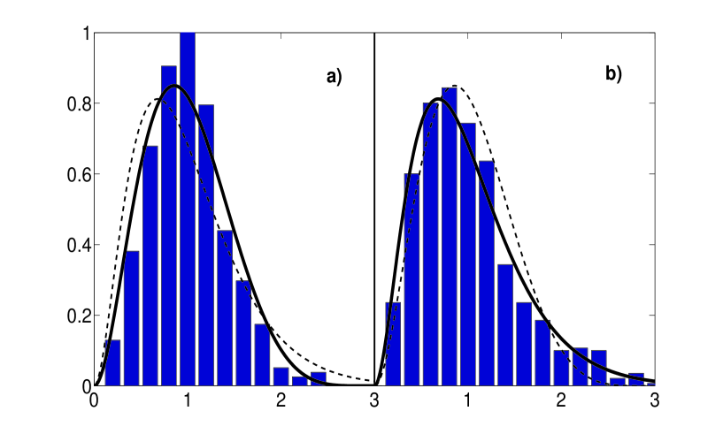
Figure 1: The measured distance distributions for cars parking on the the street $1$ and $2$ in the city of Hradec Kralove are compared with the prediction of the formula (13). The results for the street $1$ and $2$ are plotted on the panels a) and b) respectively. Bars mark the probability density extracted from the collected data. The full line stays for the formula (13) with $N=3$ (panel a)) and N=20 (panel b)). To guide the eyes the result of (13) for $N=20$ and $N=3$ are plotted on the panels a) and b) as a dashed line.

The difference between the results is not large but it is nevertheless clearly visible (compare the full and dashed lines).

To summarize we have shown that the clearance distribution for the cars parked in paralel can be described as a marginal distribution of the multivariate Dirichlet distribution with a parameter $g$. The parameter is fixed to $g=3$ by the psychophysically estimated time to collision during the parking maneuver. The measured data support this hypothesis. The theory leads further to a prediction that the clearance distribution depends on the length of the used parking segment. Also this fact is verified by the collected data.

Acknowledgement: The research was supported by the Czech Ministry of Education within the project LC06002. I appreciate the stimulating discussions with Balint Virag. The help of the PhD. students Michal Musilek and Jan Fator, who collected the parking data, is also gratefully acknowledged.

References

- [1] Renyi A.: Publ. Math. Inst. Hung. Acad. Sci. 3 (1958) 109.
- [2] Evans J.W.: Rev.Mod.Phys. 65 (4) (1993) 1281-1330
- [3] Cadilhe A.,, Araujo N.A.M. and Privman V.: J.Phys. Cond. Mat. 19 (2007) 065124
- [4] Araujo N.A.M., Coadilhe A.: Phys. Rev. E 73 (2006) 051602
- [5] D Orsogna M.R., Chou T.: J.Phys.A. 38 (2005) 531-542
- [6] Yang X.F., Knowles K.M.: J.Am.Ceram.Soc. 75 (1992) 141-147
- [7] Mackenzie J.K.: J.Chem.Phys. 37 (1962) 723-728
- [8] Rawal S., Rodgers G.J.: Physica A 246 (2005) 621-630
- [9] Seba P.: J.Phys.A 41 (2008) 122003
- [10] Bertoin J.: Random Fragmentation and Coagulation Processes. Cambridge University Press, Cambridge, 2006.
- [11] Dufresne D.: Adv. Appl. Math. 20 (1998) 285-299
- [12] Devroye L. and Neininger R.: Advances of Applied Probability, vol. 34 (2002) 441-468.
- [13] Wilks, S.S.: Mathematical Statistics. John Wiley Sons, New York
- [14] Jacobs R.A.: Trends in Cognitive Sciences Vol.6 No.8 (2002) 345
- [15] Lee, D. N.: A theory of visual control of braking based on information about time-to-collision. Perception 5 (1976), 437 459.
- [16] van der Weel F.R., van der Meer L.H., Lee N.D.: Human Movement Science 15 (1996) 253-283
- [17] Hopkins B.,Churchill A., Vogt S., Ronnqvist L.: Journal of Motor Behavior 36, Number 3 (2004) 3 - 12
- [18] Schrater P.R., Knill D.C., Simoncelli E.P.: Nature 410 (2001) 816
- [19] Farrow K., Haag J. and Borst A.: Nature Neuroscience 9 (2006) 1312 - 1320
- [20] Fajen B.R.: Journal of Experimental Psychology 31, No. 3 (2005) 480 501