The $E_{\rm peak}-E_{\rm iso}$ plane of long Gamma Ray Bursts and selection effects

Abstract

We study the distribution of long Gamma Ray Bursts in the $E_{\rm peak}-E_{\rm iso}$ and in the $E^{\rm obs}_{\rm peak}$–Fluence planes through an updated sample of 76 bursts, with measured redshift and spectral parameters, detected up to September 2007. We confirm the existence of a strong rest frame correlation $E_{\rm peak}\propto E_{\rm iso}^{0.54\pm 0.01}$. Contrary to previous studies, no sign of evolution with redshift of the $E_{\rm peak}-E_{\rm iso}$ correlation (either its slope and normalisation) is found. The 76 bursts define a strong $E^{\rm obs}_{\rm peak}$–Fluence correlation in the observer frame ($E^{\rm obs}_{\rm peak}\propto F_{\rm bol}^{0.32\pm 0.05}$) with redshifts evenly distributed along this correlation. We study possible instrumental selection effects in the observer frame $E^{\rm obs}_{\rm peak}$–Fluence plane. In particular, we concentrate on the minimum peak flux necessary to trigger a given GRB detector (trigger threshold) and the minimum fluence a burst must have to determine the value of $E^{\rm obs}_{\rm peak}$ (spectral analysis threshold). We find that the latter dominates in the $E^{\rm obs}_{\rm peak}$–Fluence plane over the former. Our analysis shows, however, that these instrumental selection effects do not dominate for bursts detected before the launch of the Swift satellite, while the spectral analysis threshold is the dominant truncation effect of the Swift GRB sample (27 out of 76 events). This suggests that the $E^{\rm obs}_{\rm peak}$–Fluence correlation defined by the pre–Swift sample could be affected by other, still not understood, selection effects. Besides we caution about the conclusions on the existence of the $E^{\rm obs}_{\rm peak}$–Fluence correlation based on our Swift sample alone

1 Introduction

One of the properties of long Gamma Ray Bursts (GRBs) that remains mysterious, but potentially fundamental for understanding their physics, is the observed correlation between the bolometric energy $E_{\rm iso}$ emitted during their prompt emission and the the peak of the spectrum $E_{\rm peak}$ in a $\nu F_{\nu}$ plot. In the observer frame a correlation between the total fluence and $E_{\rm peak}$ was found by Lloyd, Petrosian & Mallozzi (2000, LPM00 hereafter) with a sample of BATSE bursts without measured redshifts. In their pioneering work, LPM00 predicted the existence of an intrinsic $E_{\rm peak}\propto E_{\rm iso}^{a}$ correlation with $a\in[0.47,0.62]$. Later, Amati et al. (2002) indeed found such a correlation, based on a sample of 12 GRBs observed by the BeppoSAX satellite and with spectroscopically measured redshifts. The following updates (e.g. Lamb, Donaghy & Graziani 2005; Amati 2006; Ghirlanda et al. 2007) confirmed this correlation and showed that the exponent depends somewhat on the fitting method and on the sample under consideration, but is of the order of $a\sim 0.5$.

The current debate about the $E_{\rm peak}-E_{\rm iso}$ correlation concerns (a) the very existence of the correlation and the presence of outliers; (b) the evolution with redshift of the slope and normalisation of the correlation and (c) the presence of selection effects on this correlation.

The real existence of the Amati correlation has been questioned by Nakar & Piran (2005) and Band & Preece (2005) who considered different samples of GRBs, detected by BATSE, of known $E_{\rm peak}$ but without redshift determination. By considering all possible redshifts, they claimed that a large fraction of GRBs were in any case outliers to the original (Amati et al. 2002) Amati relation. They also claimed that the $E_{\rm peak}-E_{\rm iso}$ correlation was a boundary of a larger dispersion of points in the rest frame $E_{\rm peak}-E_{\rm iso}$ plane. Ghirlanda et al. (2005), using a large sample of 442 GRBs with pseudo–redshifts determined by the lag–luminosity relation (Norris, Marani & Bonnell 2000; Norris 2002; Band & Preece 2005), found that $E_{\rm peak}$ and $E_{\rm iso}$ strongly correlate. The correlation has a normalisation and scatter slightly larger than in the original Amati et al. (2002) paper. Although these pseudo–redshifts are based on the still uncertain lag–luminosity correlation, they could be used to show that there is no outlier of the $E_{\rm peak}-E_{\rm iso}$ correlation within the used sample of 442 GRB. Similar conclusions were reached by Bosnjak et al. (2007), using a different method. Consider that in all cases two GRBs (GRB 980425 and GRB 031203) were not included in the fits, being clear outliers of the correlation and also anomalous in many ways, even if there have been attempts to make them mainstream by considering them off–axis events (Ramirez–Ruiz et al. 2005), or sources whose prompt flux is dimmed by some scattering material, or spectral evolution (Ghisellini et al. 2006).

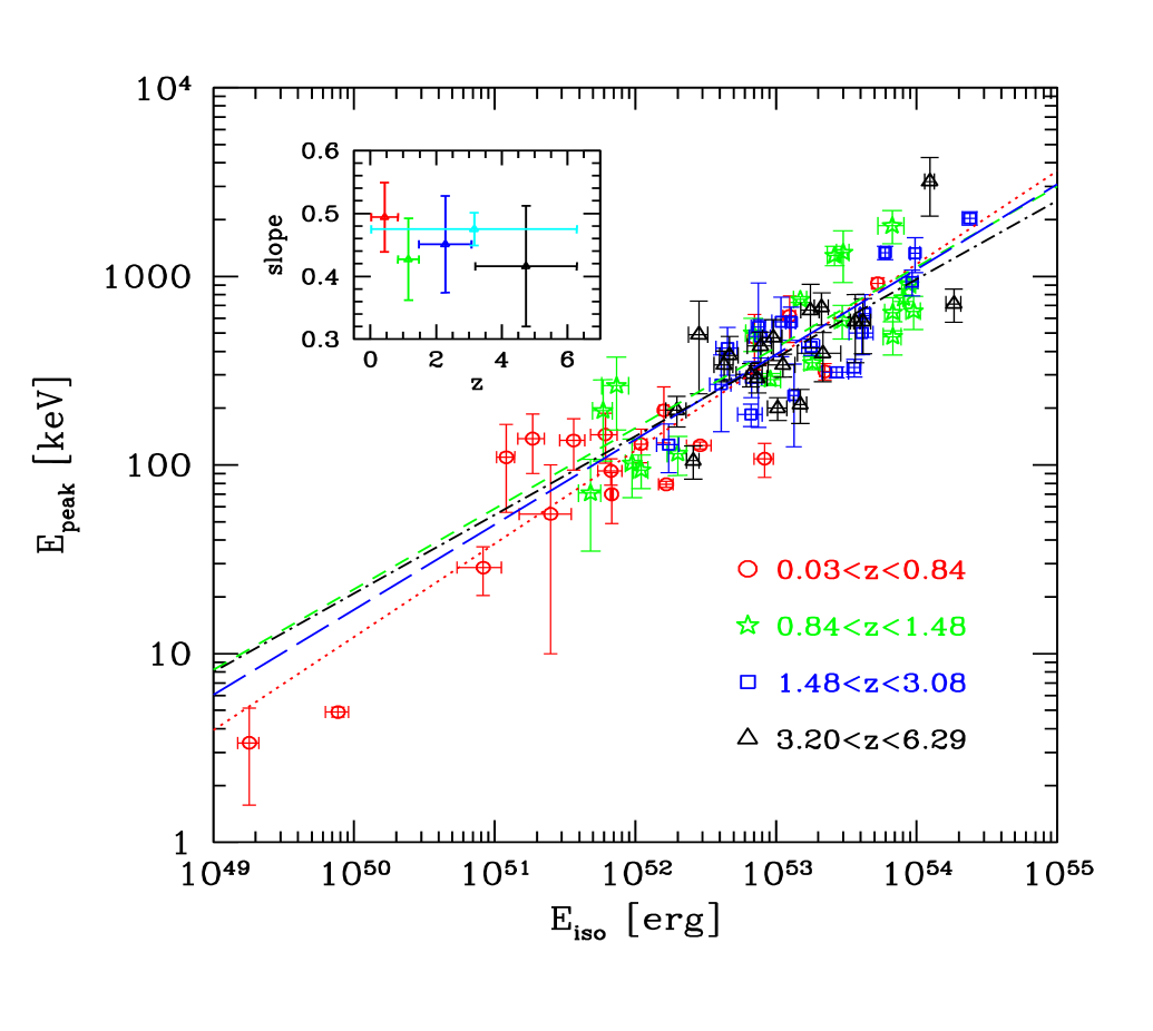
Figure 1: The 76 GRBs with known redshifts and well measured spectral properties (updated to September 2007) in the rest frame plane. Bursts are divided in four redshift bins (as labelled). The lines are the best fit obtained with the least squares method (dotted, short–dashed, long–dashed, dot–dashed from small to high redshift values, respectively). The insert represents the slope as a function of the 4 redshift bin. The slope of the correlation defined with the entire sample of 76 bursts is also shown (cyan symbol in the insert).

Li (2007, hereafter L07), considering a sample of 48 GRBs (from Amati 2006; 2007) investigated if the correlation evolves with redshift, finding that it does, becoming steeper (i.e. larger $a$) at higher redshifts.

Very recently, Butler et al. (2007, hereafter B07) claimed that the correlation exists, but it is probably the result of a selection effect, similar to the correlations often found when considering flux limited samples and calculating the correlation between the luminosities in different bands. They suggest that by multiplying the fluence and the observed peak energy by strong function of redshift can induce a correlation in the rest frame.

In this work we study these issues by updating the sample of bursts with known redshifts (§2). We study the evolution of the $E_{\rm peak}-E_{\rm iso}$ correlation with redshift in §3. In §4 we show the existence of a strong $E^{\rm obs}_{\rm peak}$–Fluence correlation. The GRB sample considered is heterogeneous in terms of the instruments that detected the bursts. This requires a deteailed analysis of the possible selection effects in order to understand if the $E_{\rm peak}-E_{\rm iso}$ correlation is an intrinsic correlation or if it is due to any selection effect. We study the instrumental selection effects in the $E^{\rm obs}_{\rm peak}$–Fluence observer frame and discuss their impact on the $E_{\rm peak}-E_{\rm iso}$ correlation (§4). The relation between the $E^{\rm obs}_{\rm peak}$–Fluence and the $E_{\rm peak}-E_{\rm iso}$ relation is briefly discussed in §5, and in §6 we draw our conclusions.

In this work we focus on the sample of bursts with measured redshifts and well defined spectral properties in order to study the issue of the redshift evolution (L07) and the selection effects on the $E_{\rm peak}-E_{\rm iso}$ correlation (see also B07). We will study the observer frame $E^{\rm obs}_{\rm peak}$–Fluence plane with larger samples of bursts of unknown $z$ in a forthcoming paper (Nava et al. in preparation).

We use $H_{0}=70$ km s^-1 Mpc^-1, $\Omega_{\rm M}=0.3$ and $\Omega_{\Lambda}=0.7$.

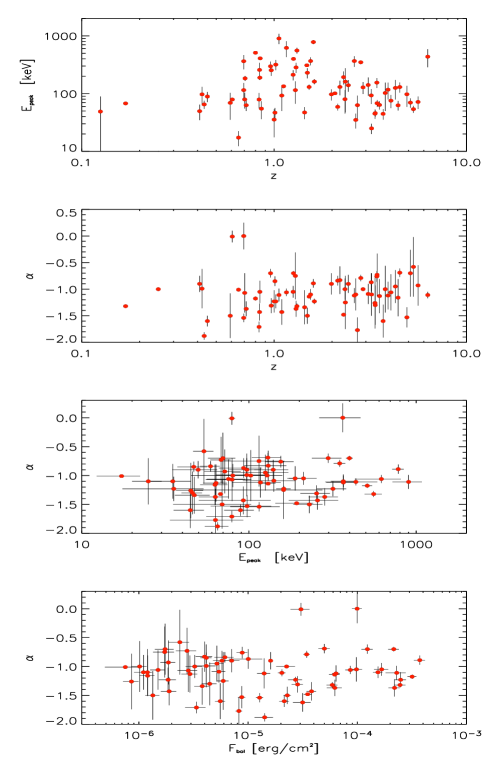
Figure 2: Correlation of the spectral parameters ($E^{\rm obs}_{\rm peak}$and $\alpha$) with redshift (top panels) and between the spectral parameters (bottom left) and the fluence (bottom right) for the sample of bursts with known redshift reported in Tab. 1.

Figure 3: Evolution of the slope of the $E_{\rm peak}-E_{\rm iso}$ correlation (defined as $E_{\rm iso}\propto E_{\rm peak}^{1/a}$ with redshift. The circles are the results obtained with the 48 GRBs of the L07 sample and the open stars are the results obtained with the 76 GRBs of our sample. The fit were performed by weighting for the erros on both $E_{\rm peak}$ and $E_{\rm iso}$ for consistency with the method adopted by L07.

2 The $E_{\rm peak}-E_{\rm iso}$ plane

The information required to put a GRB on the $E_{\rm peak}-E_{\rm iso}$ plane are (i) the redshift, (ii) the spectral parameters and (iii) the fluence. These are used to compute the bolometric isotropic energy $E_{\rm iso}$ (e.g. see Ghirlanda, Ghisellini & Lazzati 2004) and the rest frame peak energy $E_{\rm peak}$ of the $\nu F_{\nu}$ spectrum. Note that the fluence and peak energy are of the time integrated spectrum, i.e. integrated over the total duration of the burst.

We have collected all bursts with spectroscopically measured redshift and with known spectral properties. 35 GRBs were detected by instruments on-board different satellites (CGRO, BeppoSAX, Hete–II) before the Swift satellite was launched in Nov. 2004 (Gehrels et al. 2004) and 41 events were detected by different satellites (Konus–Wind, Swift, RHESSI, Suzaku, Hete–II ) since the end of 2004 in the so called “Swift era”. Among the latter in 27 cases the spectral parameters (peak energy and fluence) were derived from the analysis of the Swift–BAT data. For 19 out of 27 bursts the spectral parameters were taken from the compilation of Cabrera et al. 2007 (hereafter C07) and for the other 8 bursts the spectral parameters are from the literature. We refer to this sample of 27 bursts as the “Swift burst sample” and define the sample of all the other 49 bursts the non–Swift sample.

In Tab. 1 we report the redshifts, spectral properties and isotropic energy of the sample of the 76 GRBs. This is the most updated sample of bursts with published redshift, $E_{\rm peak}$ and fluence that can be put in the $E_{\rm peak}-E_{\rm iso}$ plane up to September 2007. For many bursts the time integrated spectrum was fitted with the Band model (Band et al. 1993) or with a cutoff power–law. There are indications (e.g. Kaneko et al. 2006, hereafter K06) that if a sufficiently broad energy range is covered by the available spectrum (e.g. up to few MeV), the time integrated spectrum is preferentially represented by the Band model. In order to uniformly estimate $E_{\rm iso}$, following Ghirlanda et al. (2007), for those bursts with a spectrum fitted by a cutoff power–law we computed the logarithmic average of $E_{\rm iso}$ derived with this model and the value derived with the Band function by fixing the high energy spectral index to –2.3 (i.e. the typical value reported in e.g. K06). For the GRBs taken from C07, $E_{\rm peak}$ was transformed into linear (and its error symmetrized), in order to have the same format of several other tables already published in the literature. Note however that for the points discussed below, our fits do not weight for the errors on the variables. All the burst before 2005 taken from Amati (2006) are corrected for the different assumption on $H_{0}$ (Amati 2006 used $H_{0}=65$ km s^-1 Mpc^-1).

In Fig. 1 we show the correlation defined by the 76 bursts listed in Tab. 1. Statistical analysis gives a Kendall’s tau correlation coefficient $\tau=0.68$ (18$\sigma$ significance). The correlation can be modelled with a power law. Actually, different fitting procedures have been adopted in the literature: (a) simple least square fit which minimizes the difference between the the data points and the model (along the ordinate direction) without wighting for the errors of the data points or (b) a fit that weights for the errors on both variables (see e.g. Press et al. 1986). The least square fit gives $\log E_{\rm peak}=(-22.59\pm 1.39)+\log E_{\rm iso}^{0.47\pm 0.03}$ with a $\chi^{2}=3.49$. The fit obtained by weighting for the errors is $\log E_{\rm peak}=(-26.66\pm 0.46)+\log E_{\rm iso}^{0.55\pm 0.01}$ with a $\chi^{2}=545$ for 74 degrees of freedom. In the latter case, the reduced $\chi^{2}$ is extremely large and this is due to the sample dispersion (see below) which is much larger than the statistical errors associated with the variables. Such a large $\chi^{2}$ also leads to underestimate the errors of the parameters of the fit. It has been proposed (Reichart et al. 2001, 2005, but see Guidorzi et al. 2005, see also D’agostini et al. 2006) that the fit should account for an additional parameter which is the sample variance. Amati (2006) performed this fit on his GRB sample and found a quite large value of the sample variance $\sigma=0.15$. Instead, we proposed (Ghirlanda et al. 2004, see also Liang & Zhang 2005) that the large dispersion of the data points in the $E_{\rm peak}-E_{\rm iso}$ plane is due to a third observable, i.e. the jet break time. Indeed, by correcting the isotropic energy for the collimation angle that can be derived from the jet break time of the optical light curve, the dispersion of the $E_{\rm peak}-E_{\rm iso}$ correlation is greatly reduced (Ghirlanda et al. 2007, Nava et al. 2007). In this work we will adopt the least square fitting method (Press et al. 1986 p.499) without weighting for the errors on the variables because the sample dispersion in the $E_{\rm peak}-E_{\rm iso}$ plane defined by the 76 GRBs ($\sigma$=0.22 - consistent with the values found with smaller GRB samples, e.g. Ghirlanda et al. 2004, 2005; Amati et al. 2006, C07) is clearly larger than the typical statistical errors associated with either $E_{\rm peak}$ and $E_{\rm iso}$($\langle\sigma_{logE_{\rm p}}\rangle=0.1$ and $\langle\sigma_{logE_{\rm iso}}\rangle=0.06$).

With the most updated sample of 76 GRBs reported in Tab. 1 we can also verify that no correlation exists between the spectral parameters or with the redshift (see Fig. 2). In particular, there is no correlation between $\alpha$ and $z$ nor between $\alpha$ and $E^{\rm obs}_{\rm peak}$(second and third panel in Fig. 2). A different, strong, correlation between $\alpha_{\rm pl}$ of the fit with a single power law and the peak energy of the fit with a cutoff–power law has been reported recently (Sakamoto et al. 2006; Butler et al. 2007) from the analysis of the Swift-BAT spectra. Note that in this correlation the two spectral parameters $\alpha_{\rm pl}$ and $E^{\rm obs}_{\rm peak}$ belong to two different models, i.e. a single power law and a cutoff–power law model, respectively. However, it has been shown in C07 that this correlation is spurious (Fig. 3 and Sec. 3.2 of that paper). Although a correlation indeed appears between the single power law spectral index $\alpha_{pl}$ and $E^{\rm obs}_{\rm peak}$ (of the cutoff–power law model – see bottom panel of Fig. 3 in C07), it has no physical meaning: it is the result of the attempt of the single power law model fit to account for the spectral data above the peak which have a smaller $\nu F_{\nu}$ flux. Spectra with lower $E^{\rm obs}_{\rm peak}$ will have a larger fraction of data points above the single power law fit and they will cause the fit with the single power law to be softer. This accounts for the observed positive correlation. It is then dangerous to use this correlation for those cases where $E^{\rm obs}_{\rm peak}$ is not measured, to derive it on the basis of $\alpha_{pl}$.

Recently B07 derived the spectral properties of almost all the bursts detected by Swift through a Bayesian method. The method proposed in B07 to estimate the peak energy, far outside the energy range of BAT/Swift (15–150 keV) is based on the assumption of a prior distribution for the observed peak energy which is the (gaussian) peak energy distribution of BATSE bright bursts (Kaneko et al. 2005), for $E^{\rm obs}_{\rm peak}$$>$300 keV, and a uniform distribution for energies below this value. However, as also noted by B07, from the comparison of these estimates of $E^{\rm obs}_{\rm peak}$ with those derived from the spectral fits of the Konus-Wind and Suzaku, for the common bursts, there could be a bias at high values of $E^{\rm obs}_{\rm peak}$ estimated from Swift data through the Bayesian method and this could influence the findings of B07.

In this paper, we adopt a conservative approach and we consider only the Swift GRBs for which the estimates of the peak energy is based on a standard (i.e. frequentist) fit of the BAT spectra of bursts with known redshifts (from C07).

3 No redshift evolution of the $E_{\rm peak}-E_{\rm iso}$ correlation

The 76 bursts of Tab. 1 are distributed in a large redshift range, up to $z=6.3$ (for GRB 050904 – Tagliaferri et al. 2005). It is worth to investigate if any evolution with $z$ can affect the $E_{\rm peak}-E_{\rm iso}$ correlation defined by this sample. Note that the simple evolution of the burst energetics ($E_{\rm iso}$) with $z$ does not necessarily implies the evolution of the $E_{\rm peak}-E_{\rm iso}$ correlation. Indeed, if $E_{\rm peak}$ evolves in the same way as $E_{\rm iso}$ (i.e. if the link between $E_{\rm iso}$ and $E_{\rm peak}$ is physically robust) then we should see no evolution of the slope and normalisation of the $E_{\rm peak}-E_{\rm iso}$ correlation with $z$.

The possible redshift evolution of the $E_{\rm peak}-E_{\rm iso}$ correlation has been investigated by Li 2007 (L07, hereafter). He used the sample of 48 GRBs (from Amati 2006, 2007), restricting to long events and excluding the peculiar GRB060614 (Gherels et al. 2006) and dividing the sample into 4 redshift bins. Comparing the slopes of the correlation corresponding to each redshift bin he found that the $E_{\rm peak}-E_{\rm iso}$ correlation becomes steeper for increasing redshift. Note that the slope defined by L07 refers to the $E_{\rm iso}\propto E_{\rm peak}^{1/a}$ correlation, i.e. the reverse of that defined in this paper. This is opposite to what one naively expects, namely that for larger $z$ we select, on average, more energetic bursts with the same $E_{\rm peak}$, resulting in a flattening of the $E_{\rm peak}-E_{\rm iso}$ slope. Note also from Fig. 1 that bursts with different redshifts are distributed along the $E_{\rm peak}-E_{\rm iso}$ correlation with no evident segregation along the correlation itself (except for the excess of low redshift bursts in the low end of the $E_{\rm peak}-E_{\rm iso}$ plane).

In our study we examine first the possible evolution with redshift of the $E_{\rm peak}-E_{\rm iso}$ correlation defined as $E_{\rm peak}\propto E_{\rm iso}^{a}$. Our sample of Tab. 1 extends the original sample of 48 GRBs, used by L07, both in number and redshift. To verify his results, we have divided the 76 GRB sample into four redshift bins, chosen to have an equal number of 19 bursts per bin. These $z$ bins are very similar to those adopted by L07. We fit the $E_{\rm peak}-E_{\rm iso}$ correlation in each sub–sample through the least square method (see Sec. 2). The results are shown in the insert of Fig. 1. The analysis of the $E_{\rm peak}-E_{\rm iso}$ correlation in each redshift bin excludes the evolution of the slope of the $E_{\rm peak}-E_{\rm iso}$ correlation with $z$, given the present sample of 76 events. Indeed, the slopes of the $E_{\rm peak}-E_{\rm iso}$ correlations defined by the four redshift sub–samples are consistent among themselves and also with the slope of the correlation defined by the entire sample (insert of Fig. 1). We have also verified that the normalisation of the correlations defined by the four redshift bins are consistent.

We then investigated the possible reasons for the discrepancy of our results with respect to L07. We reconstructed the sample of 48 GRBs used by L07 (with data taken from Amati et al. 2006, 2007). Using this sub–sample we find the same results of Li (2007), concerning the evolution of the slope and normalization of the $E_{\rm peak}-E_{\rm iso}$ correlation with redshift (circles in Fig. 3). However, when extending this sample to the 76 GRBs of our present sample, we do not find any evolution with redshift (star symbols in Fig. 3). Note that for this comparison we used the same fitting method of L07, which weights for the errors on both variables, and fitted the $E_{\rm iso}\propto E_{\rm peak}^{1/a}$ correlation. We then conclude that the Li (2007) results were affected by too low statistics, and that there is no evidence that the $E_{\rm peak}-E_{\rm iso}$ correlation evolves.

GRB	$z$	$\alpha$	$\beta$	Fluence	Range	$E_{\rm peak}$	$E_{\rm iso}$	Ref
				erg cm-2	keV	keV	erg
970228	0.695	$-$1.54 [0.08]	$-$2.5 [0.4 ]	1.1e–5 [0.1e–5]	40–700	195 [64]	1.60e52 [0.12e52]	1
970508a	0.835	$-$1.71 [0.1 ]	$-$2.2 [0.25 ]	1.8e–6 [0.3e–6]	40–700	145 [43]	6.12e51 [1.3e51]	1
970828	0.958	$-$0.70 [0.08]	$-$2.1 [0.4 ]	9.6e–5 [0.9e–5]	20–2000	583 [117]	2.96e53 [0.35e53]	2
971214	3.42	$-$0.76 [0.1 ]	$-$2.7 [1.1 ]	8.8e–6 [0.9e–6]	40–700	685 [133]	2.11e53 [0.24e53]	1
980326	1.0	$-$1.23 [0.21]	$-$2.48 [0.31 ]	7.5e–7 [1.5e–7]	40–700	71 [36]	4.82e51 [0.86e51]	1
980613	1.096	$-$1.43 [0.24]	$-$2.7 [0.6 ]	1.e–6 [0.2e–6]	40–700	194 [89]	5.9e51 [0.95e51]	1
980703	0.966	$-$1.31 [0.14]	$-$2.39 [0.26 ]	2.3e–5 [0.2e–5]	20–2000	499 [100]	6.90e52 [0.82e52]	3
990123	1.600	$-$0.89 [0.08]	$-$2.45 [0.97 ]	3.e–4 [0.4e–4]	40–700	2031 [161]	2.39e54 [0.28e54]	1
990506	1.30	$-$1.37 [0.15]	$-$2.15 [0.38 ]	1.9e–4 [0.2e–4]	20–2000	653 [130]	9.5e53 [1.13e53]	2
990510	1.619	$-$1.23 [0.05]	$-$2.7 [0.4 ]	1.9e–5 [0.2e–5]	40–700	423 [42]	1.78e53 [0.26e53]	1
990705	0.843	$-$1.05 [0.21]	$-$2.2 [0.1 ]	7.5e–5 [0.8e–5]	40–700	348 [28]	1.82e53 [0.23e53]	1
990712	0.433	$-$1.88 [0.07]	$-$2.48 [0.56 ]	6.5e–6 [0.3e–6]	40–700	93 [15]	6.72e51 [1.29e51]	1
991208	0.706	… …	…. …	1.6e–4 [5.0e–6]	20–10000	313 [31]	2.23e53 [0.18e53]	5
991216	1.02	$-$1.23 [0.13]	$-$2.18 [0.39 ]	1.9e–4 [0.2e–4]	20–2000	642 [129]	6.75e53 [0.81e53]	2
000131	4.50	$-$0.69 [0.08]	$-$2.07 [0.37 ]	4.2e–5 [0.4e–5]	20–2000	714 [142]	1.84e54 [0.22e54]	2
000210	0.846	… …	…. …	7.6e–5 [5.0e–6]	20–10000	753 [26]	1.49e53 [0.16e53]	5
000418	1.12	… …	…. …	2.6e–6 [4.0e–5]	20–10000	284 [21]	0.91e53 [0.17e53]	5
000911	1.06	$-$1.11 [0.12]	$-$2.32 [0.41 ]	2.2e–4 [0.2e–4]	15–8000	1856 [371]	6.7e53 [1.4e53]	5
000926	2.07	… …	…. …	2.6e–5 [4.e–6]	20–2000	310. [20]	2.7e53 [0.58e53]	5
010222	1.48	… …	…. …	1.4e–4 [8.e–6]	20–2000	766 [30]	8.1e53 [0.86e52]	5
010921	0.45	$-$1.60 [0.1 ]	…. …	1.84e–5 [0.1e–5]	2–400	129. [26]	1.1e52 [0.11e52]	5
011211b	2.140	$-$0.84 [0.09]	…. …	2.6e–6 [0.3e–6]	40–700	185 [25]	6.64e52 [1.32e52]	(7) 2
020124	3.198	$-$0.87 [0.17]	$-$2.6 [0.65 ]	8.1e–6 [0.9e–6]	2–400	390 [113]	2.15e53 [0.73e53]	8
020405	0.695	$-$0.00 [0.25]	$-$1.87 [0.23 ]	7.4e–5 [0.7e–5]	15–2000	617 [171]	1.25e53 [0.13e53]	2
020813b	1.255	$-$1.05 [0.11]	…. …	1.0e–4 [0.1e–4]	30–400	478 [95]	6.77e53 [1.00e53]	3
020819B	0.41	$-$0.90 [0.15]	$-$2.0 [0.35 ]	8.8e–6 [9.e–7]	2–400	70. [21]	6.8e51 [0.17e51]	(7) 5
020903b	0.25	$-$1.00 [0.0 ]	… …	5.9e–8 [1.4e–8]	2–10	3.37 [1.79]	1.8d49 [0.31d49]	9
021004b	2.335	$-$1.00 [0.2 ]	…. …	2.6e–6 [0.6e–6]	2–400	267 [117]	4.09e52 [0.71e52]	7
021211	1.01	$-$0.85 [0.09]	$-$2.37 [0.42 ]	2.2e–6 [0.2e–6]	30–400	94 [19]	1.1e52 [0.13e52]	2
030226b	1.986	$-$0.90 [0.2 ]	…. …	5.6e–6 [0.6e–6]	2–400	290 [63]	6.7e52 [1.20e52]	7
030328	1.520	$-$1.14 [0.03]	$-$2.1 [0.3 ]	3.7e–5 [0.14e–5]	2–400	328 [35]	3.61e53 [0.40e53]	3
030329	0.169	$-$1.32 [0.02]	$-$2.44 [0.08 ]	1.2e–4 [0.12e–4]	3–400	79 [3]	1.66e52 [0.20e52]	3
030429b	2.656	$-$1.10 [0.3 ]	… …	8.5e–7 [1.4e–7]	2–400	128 [37]	1.73e52 [0.31e52]	7
040924c	0.859	… …	…. …	2.6e–6 [0.0]	30–400	102 [35]	0.95e52 [0.1e52]	5
041006b	0.716	$-$1.37 [0.14]	… …	2.0e–5 [0.2e–5]	25–100	108 [22]	8.30e52 [1.3e52]	3
050126b	1.29	$-0$.75 [0.44]	… …	8.55e–7 [1.82e–7]	15–150	263 [110]	7.36e51 [1.60e51]	10
050223d,b	0.5915	$-$1.50 [0.42]	… …	6.14e–7 [0.83e–7]	15–150	110 [54]	1.21e51 [1.77e50]	10
050318b	1.44	$-$1.34 [0.32]	… …	2.1e–6 [0.2e–7]	15–350	115 [27]	2.00e52 [0.31e52]	11
050401e	2.9	$-$1.00 [0.0 ]	$-$2.45 …	1.93e–5 [0.04e–5]	20–2000	501 [117]	4.1e53 [0.8e53]	13
050416A	0.653	$-$1.01 [0.0 ]	$-$3.4 …	3.5e–7 [0.3e–7]	15–150	28.6 [8.3]	8.3e50 [2.9e50]	14
050505b	4.27	$-$0.95 [0.31]	… …	2.58e–6 [3.06e–7]	15–150	661 [245]	1.76e53 [2.61e52]	10
050525Ab	0.606	$-$0.01 [0.11]	…. …	2.01e–5 [0.05e–5]	15–350	127 [5.5]	2.89e52 [0.57e52]	25
050603	2.821	$-$0.79 [0.06]	$-$2.15 [0.09]	3.41e–5 [0.06e–5]	20–3000	1333 [107]	5.98e53 [0.4e53]	15
050803b	0.422	$-$0.99 [0.37]	… …	2.08e–6 [2.57e–7]	15–150	138 [48]	1.86e51 [3.99e50]	10
050814b	5.3	$-$0.58 [0.56]	… …	1.46e–6 [1.16e–7]	15–150	339 [47]	1.12e53 [2.43e52]	10
050820Ab	2.612	$-$1.12 [0.14]	… …	5.27e–5 [1.2e–5]	20–1000	1325 [277]	9.75e53 [0.77e53]	16
050904	6.29	$-$1.11 [0.06]	$-$2.2 [0.4]	5.4e–6 [1.e–7]	15–150	3178 [1094]	1.24e54 [0.1e54]	26
050908b	3.344	$-$1.26 [0.48]	… …	4.36e–7 [0.46e–7]	15–150	195 [36]	1.97e52 [3.21e51]	10
050922Cb	2.198	$-$0.83 [0.26]	…. …	2.6e–6 [0.26e–6]	30–400	417 [118]	4.53e52 [0.78e52]	17
051022b	0.80	$-$1.17 [0.038]	…. …	2.61e–4 [0.8e–4]	20–2000	918 [63]	5.3e53 [0.5e53]	27
051109Ab	2.346	$-$1.25 [0.5 ]	…. …	4.0e–6 [1.0e–6]	20–500	539 [381]	7.52e52 [0.88e52]	18
060115b	3.53	$-$1.13 [0.32]	… …	1.6e–6 [1.07e–7]	15–150	288 [47]	7.38e52 [1.23e52]	10
060124b	2.297	$-$1.48 [0.02]	… …	2.5e–5 [0.35e–5]	20–2000	636 [162]	4.3e53 [0.34e53]	19
060206b	4.048	$-$1.06 [0.34]	…. …	8.4e–7 [0.4e–7]	15–150	381 [98]	4.68e52 [0.71e52]	20
060210b	3.91	$-$1.12 [0.26]	… …	6.92e–6 [3.74e–7]	15–150	575 [186]	4.15e53 [5.7e52]	10
060218b	0.0331	$-$1.62 [0.16]	… …	3.7e–6 [0.37e–6]	15–150	4.9 [0.3]	7.7e49 [1.42e49]	29 (31)
060223Ab	4.41	$-$1.16 [0.35]	… …	6.54e–7 [0.52e–7]	15–150	339 [63]	4.29e52 [6.64e51]	10
060418b	1.489	$-$1.50 [0.15]	… …	1.6e–5 [0.16e–5]	20–1100	572 [114]	1.28e53 [0.10e53]	21
060510Bb	4.9	$-$1.53 [0.19]	…. …	3.86e–6 [2.88e–7]	15–150	575 [227]	3.67e53 [2.87e52]	10
060522b	5.11	$-$0.70 [0.44]	…. …	1.05e–6 [1.04e–7]	15–150	427 [79]	7.77e52 [1.52e52]	10

Table 1: continue….

GRB	z	$\alpha$	$\beta$	Fluence	Range	$E_{\rm peak}$	$E_{\rm iso}$	Ref
				erg cm-2	keV	keV	erg
060526f	3.21	$-$1.1 [0.4 ]	$-$2.2 [0.4]	4.9e–7 [0.6e–7]	15–150	105.25 [21.1]	2.58e52 [0.26e52]	26
060605b	3.78	$-$1.0 [0.44]	… …	5.33e–7 [1.12e–7]	15–150	490 [251]	2.83e52 [4.5e51]	10
060607Ab	3.082	$-$1.09 [0.19]	… …	2.49e–6 [1.58e–7]	15–150	575 [200]	1.09e53 [1.55e52]	10
060614	0.125	$-$10 [0 ]	… …	2.2e–5 [0.22e–5]	15–150	55 [45]	2.51e51 [1.0e51]	28
060707b	3.43	$-$0.73 [0.4 ]	… …	1.63e–6 [1.13e–7]	15–150	302 [42]	6.62e52 [1.39e52]	10
060714b	2.711	$-$1.77 [0.24]	… …	3.06e–6 [3.96e–7]	15–150	234 [109]	1.34e53 [9.12e51]	10
060814	0.84	$-$1.43 [0.16]	… …	2.69e–5 [0.26e–5]	20–1000	473 [155]	7.01e52 [0.7e52]	32
060904Bb	0.703	$-$1.07 [0.37]	… …	1.48e–6 [1.91e–7]	15–150	135 [41]	3.64e51 [7.43e50]	10
060906b	3.686	$-$1.6 [0.31]	… …	2.38e–6 [1.92e–7]	15–150	209 [43]	1.49e53 [1.56e52]	10
060908b	2.43	$-$0.9 [0.17]	… …	2.66e–6 [1.11e–7]	15–150	479 [110]	7.79e52 [1.35e52]	10
060927b	5.6	$-$0.93 [0.38]	… …	1.1e–6 [0.1e–6]	15–150	473 [116]	9.55e52 [1.48e52]	22
061007	1.261	$-$0.7 [0.04]	$-$2.61 [0.21]	2.5e–4 [0.15e–4]	20–10000	902 [43]	8.82e53 [0.98e53]	23
061121b	1.314	$-$1.32 [0.05]	…. …	5.7e–5 [0.4e–5]	20–5000	1289 [153]	2.61e53 [0.3e53]	24
061126b	1.1588	$-$1.06 [0.07]	… …	3.0e–5 [0.4e–5]	15–2000	1337 [410]	3.0e53 [0.3e53]	12
061222Bb	3.355	$-$1.3 [0.37]	… …	2.24e–6 [1.23e–7]	15–150	200 [28]	1.03e53 [1.6e52]	10
070125	1.547	$-$1.1 [0.1 ]	$-$2.08 [0.13]	1.74e–4 [0.17e–4]	20–10000	934 [148]	9.3e53 [0.93e53]	30

Table 1: ^a GRB 970508 is included following Amati (2006), but it was excluded in Ghirlanda et al. (2004) and Ghirlanda et al. (2007) because of the inconsistency of the BATSE and $Beppo$SAX spectrum (i.e. it is a candidate outlier if the BATSE spectrum is assumed). In the sample of bursts before 2005 there are some $E_{\rm peak}$ and $E_{\rm iso}$  values which are different from the recent compilation of Amati (2006). This is because he takes the average when two or more instruments (e.g. Konus and Hete) made the spectrum. This is correct when the spectral results are consistent, but we do not adopt the same values if the spectral results are inconsistent. ^b $E_{\rm iso}$ has been computed as the logarithmic average of the values found with the Band (with $\beta$ fixed at –2.3) and cutoff power–law model (see also Ghirlanda et al. 2007, Firmani et al. 2005). ^c We adopt the peak energy and isotropic energy values reported in Amati et al. (2006). There are only two GCNs for this burst giving the fluence and peak energy derived by Hete–II and Konus, which are consistent. We then take the average of the two values. $\alpha$ values are not given in the GCN. ^d The redshift is known but although it is present in B07 they do not report the redshift. ^e We adopt an average of the spectral properties of the two peaks reported by the GCNs. Note that the two spectra are consistent. ^f This is the burst discussed on our webpage (http://www.brera.inaf.it/utenti/gabriele/060526.html). This burst is an outlier of the Amati relation if the peak energy is much larger. References: before 2005: (1) Amati et al. (2002); (2) Ghirlanda et al. (2004, and references therein); (3) Nava et al. (2006 and references therein); (4) Ulanov et al. (2005); (5) Amati (2006 and references therein); (6) Firmani et al. (2006); (7) Sakamoto et al. (2005); (8) Atteia et al. (2005); (9) Sakamoto et al. (2004); Since 2005: (10) Cabrera et al. (2007). For the error the geometric mean is computed from the extremes of the logarithmic values); (11) Perri et al. (2005); (12) Perley et al. (2007, spectral analysis of the BAT+RHESSI spectrum); (13) Golenetskii et al. (2005); (14) Sato et al. (2005); (15) Golenetskii et al. (2005a); (16) Cenko et al. (2006); (17) Crew et al. (2005); (18) Golenetstkii et al., (2005b); (19) Romano et al. (2006); (20) Palmer et al. (2006); (21) Golenetskii et al. (2006); (22) Stamatikos et al. (2006); (23) Golenetskii et al. (2006a); (24) Golenetskii et al. (2006b, $E_{\rm peak}$ and $E_{\rm iso}$ are the average of the values found by the RHESSI and Konus spectra, while the spectral parameters are of the Konus spectrum); (25) Blustin et al. (2005); (26) Schaefer (2007); (27) Golenetskii et al. (2006c); (28) Mangano et al. (2007); (29) Campana et al. (2006); (30) Golenetskii et al. (2007). The burst was also seen by RHESSI (Bellm et al. 2007) whose spectrum is inconsistent with that of Konus. However, the two $E_{\rm peak}$ and the fluences values given in the GCN are inconsistent with the average $E_{\rm peak}$ reported in the same GCN (for RHESSI). For this reason we report and use the Konus spectral data; (31) Ghisellini et al. (2006); (32) Golenetskii et al. (2006d).

4 The $E^{\rm obs}_{\rm peak}$–Fluence correlation

The rest frame $E_{\rm peak}-E_{\rm iso}$ correlation is defined by multiplying the observed peak energy by $(1+z)$ and the observed (bolometric) fluence by $4\pi d_{\rm L}^{2}/(1+z)$, where $d_{\rm L}$ is the luminosity distance. Therefore, in principle, the $E_{\rm peak}-E_{\rm iso}$ correlation could be only apparent, being the result of multiplying $E^{\rm obs}_{\rm peak}$ and the fluence $F$ by strong functions containing the redshifts (as argued by B07).

To study if this is the case, it is necessary to study what region of the observational plane $E^{\rm obs}_{\rm peak}$–Fluence is accessible to observations. Any detector, in fact, can only observe GRBs above a limiting fluence and within a limited energy range.

Other selection effects could be related to the requirement of measuring the redshift: for instance (in the absence of X–ray lines) we require the burst to be located precisely enough to make possible the optical follow up and we also require its afterglow to be visible in the optical. If only bright bursts had an optical afterglow, this would affect the resulting correlation in the $E_{\rm peak}-E_{\rm iso}$ plane.

We focus here on the selection effects introduced by requiring that the burst is not only detected, but it must be bright enough to allow the determination of the spectrum of its prompt emission.

Consider first how our 76 GRBs with known redshift are located in the $E^{\rm obs}_{\rm peak}$–Fluence plane, as illustrated in Fig. 4. Different symbols correspond to GRBs in different redshift bins. Note that:

• These bursts define a strong correlation in this plane. The Kendall’s correlation coefficient is $\tau=0.53$ (9$\sigma$ significance). The least square fit has a slope 0.39$\pm$0.04. However, it is very likely that this correlation is affected by truncation effects which should be considered when computing the correlation strength and when recovering its “true” slope (LPM00).

• There is no segregation in redshift. We do not find that nearby bursts are brighter and bluer, and distant bursts are fainter and redder, as we would expect if there were no intrinsic correlation between $E_{\rm peak}$ and $E_{\rm iso}$.

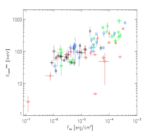
Figure 4: $E^{\rm obs}_{\rm peak}$–bolometric fluence plane for the sample of 76 bursts of Tab. 1. We show with different symbols the redshift bins corresponding to 0.03–0.843 (circles), 0.846–1.48 (stars), 1.49–3.1 (squares) and 3.2–6.29 (triangles). The least square fit to the data is $E^{\rm obs}_{\rm peak}$$\propto F_{\rm bol}^{0.4}$ where $F_{\rm bol}$ is the fluence in the energy range 1 keV – 10 MeV. The scatter of these bursts around the best fit has a $\sigma=0.21$.

The existence of a $E^{\rm obs}_{\rm peak}$–Fluence correlation is not new: it was discovered with a relatively small sample of BATSE bursts by LPM00 and subsequently confirmed with the discovery of the class of X–Ray Flashes by BeppoSAX and Hete–II (e.g. Lamb, Donaghy & Graziani 2005). Sakamoto et al. (2005) showed that a correlation between these two observables exists in the Hete–II burst sample and extends from the softest $E^{\rm obs}_{\rm peak}$ of a few keV to the few hundred keV range (e.g. Preece et al. 2000 and K06 for the BATSE sample). We will discuss the sample of bursts with no redshift, but with measured $E^{\rm obs}_{\rm peak}$, in a forthcoming paper (Nava et al. 2008, in preparation).

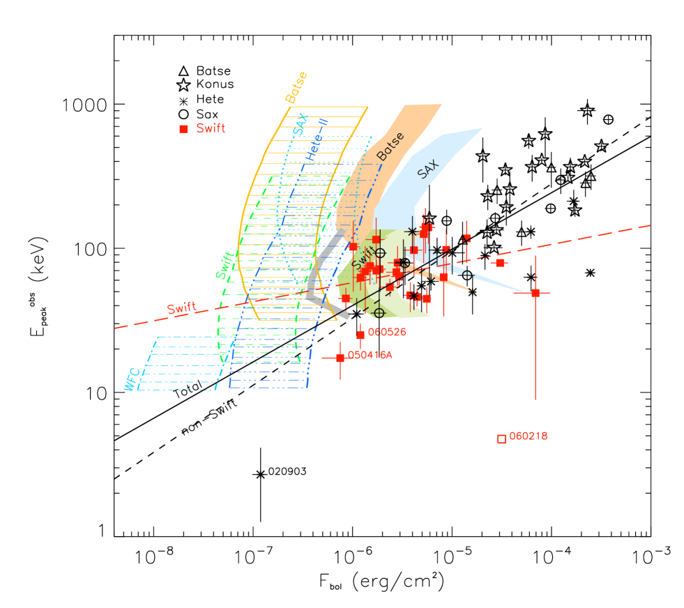
Figure 5: Observer frame plane of the peak energy and bolometric fluence (1–10⁴ keV). Bursts whose peak energy has been derived by the analysis of the BAT data are shown with filled squares. The open symbols are all the other bursts with redshift. The shades regions represent the minimum fluence that a burst can have (for different duration of the burst – 5 s and 20 s for the left and right boundary of each shaded region, respectively) in order to perform the spectral analysis and derive constraints on $E^{\rm obs}_{\rm peak}$. For Swift we also report (narrow grey stripe) the limiting curve derived by slightly different criteria (see text for details). The single lines represent the trigger sensitivity for Swift (dashed), BATSE (solid), BeppoSAX (dotted), Hete-II (triple dot–dashed). The best fit of the sample of Swift bursts (long–dashed line) and non–Swift bursts (dashed line) and of the total sample (solid line) are also reported. These fits, however, do not take into account the truncation effects (see text for details). The open red square represents GRB 060218 whose peak energy has been determined by the analysis of the Swift–XRT data (Campana et al. 2006).

4.1 Instrumental biases in the $E^{\rm obs}_{\rm peak}$–Fluence plane

Consider the two regions in the $E^{\rm obs}_{\rm peak}$–Fluence plane of Fig. 4 below and above the correlation where we have a paucity of points. Region 1 is characterized by large fluences and low/moderate $E^{\rm obs}_{\rm peak}$; region 2 comprises small fluences, large/moderate $E^{\rm obs}_{\rm peak}$. In region 1 there are no (or very few) bursts, although there is no instrumental effect against their detection. This implies that they really do not exist (or, rather, they are very few). In region 2, instead, the paucity of points in the $E^{\rm obs}_{\rm peak}$–Fluence plane could be affected by some instrumental selection effect.

The detectors (past and present) dedicated to study GRBs introduce at least two selection effects on the population of bursts that they observe: (a) the trigger sensitivity which is the ability to detect a burst as a transient event significantly above the average background (see e.g. Band 2003; 2006); (b) the “spectral analysis threshold” which is the minimum fluence required to constrain the peak energy from the spectral analysis.

For any $E^{\rm obs}_{\rm peak}$, a minimum photon flux is required to trigger the burst. This minimum flux depends on the spectral properties of the burst (especially its peak energy – e.g. Band 2003), on the detector design and on the total background rate seen by the instrument. The ability to detect a GRB for a non–imaging instruments (like BATSE, Konus, HeteII–Fregate, $Beppo$SAX–GRBM), is related to the significance of the burst intensity (i.e. its peak flux) with respect to an average background (see e.g. Band et al. 2003). For imagers this threshold is modified by the coding aperture of the mask and it can be even lower (Band 2006). The trigger sensitivity curves as a function of the burst peak spectral energy for different instruments has been computed by Band (2003) (see also Band 2006). We show them for BATSE, Swift, Hete-II, BeppoSAX in Fig. 5. These curves correspond to the sensitivity limit of each instrument to burst with a varying $E^{\rm obs}_{\rm peak}$and are computed by Band (2003) in the peak flux – peak energy space. In order to report them on our $E^{\rm obs}_{\rm peak}$–Fluence plane we have (i) to assume a typical burst duration to cumpute the fluence and (ii) to assume a burst spectrum to convert from the photon units to the energy units. To make this conversion we assumed a burst with a 1 s duration which represents a lower limit for the detection sensivity of long GRBs and we also assumed a burst with a typical Band spectrum (with $\alpha=-1.0$ and $\beta=-2.3$) and with a variable $E^{\rm obs}_{\rm peak}$. As discussed by Band 2003, however, these curves are only an estimate of the burst detection sensitivity for any given instrument because the trigger strongly depends on the burst time profile and on the background. In particular we tried to account for the unknown burst duration when converting the Band (2003) limiting curves in the fluence plane of Fig 5. In the simplest case of a burst with a single pulse with a triangular shape, the conversion is $F(E_{\rm peak})=P(E_{\rm peak})T/2$ where $F(E_{\rm peak})$ and $P(E_{\rm peak})$ are the fluence and peak flux as a function of the peak energy of the burst and $T$ is the burst duration. Under this simple hypothesis, our curves for the trigger threshold would move in the plot of Fig. 5 proportionally to $T/2$. However, GRBs light curves are all but simple single peaked triangles. A more realistic conversion factor between the peak flux and the fluence, which also accounts for the typical variation of the flux with time, can be obtained from the ratio of the fluence and the peak flux $F/P$ for the complete GRBs of the BATSE sample (taking into account only the long burst population). We found that the distribution of the ratio $F/P$ peaks at $\sim$6 and has a tail towards lower values. In Fig. 5 we report the two limiting curves for the trigger defined with a burst of duration 1 s and with the above ratio. Note that the WFC trigger thresholds are on the left of the plot and are clearly not affecting the distribution of bursts with known redshifts. Moreover, these curves are here plotted in the very narrow energy range corresponding to the WFC trigger but their behaviour at higher $E^{\rm obs}_{\rm peak}$ values has been shown to be very weak (see Fig. 3 of Band 2003). The WFC thresholds were taken from Band (2003) and they are consistent with what reported by Vetere et al. (2007). This is contrary to what one could think, i.e. that due to the requirement to accurately locate the burst in order to measure its redshift, it is the WFC trigger threshold to bias the GRBs (of the pre–Swift sample) with measured redshift in the $E^{\rm obs}_{\rm peak}$–Fluence plane (but see also the discussion at the end of this section). These results, taken at face values, imply that the distribution of GRBs of our heterogeneous sample in the $E^{\rm obs}_{\rm peak}$–Fluence plane are not affected by the trigger sensitivity of the different istruments that detected these bursts.

However, in order to perform the spectral analysis and to constrain any model parameters we also require a minimum number of total (time integrated) photons. To derive the threshold fluence $F_{\rm min}$ required to perform the spectral analysis, we have simulated several spectra with different $E^{\rm obs}_{\rm peak}$ and fluence values. For this simulation we need the detector response and a typical background spectrum. These two files are available for BATSE and Swift at the respective web sites. Unfortunately, no public response file was found for the BeppoSAX–GRBM instrument. For the Swift simulations we used the batphasimerr tool of the latest HASOFTv6.3.2 release (C. Markwardt, private communication).

We made two sets of simulations, assuming a burst durations of 5 and 20 seconds, respectively, with a corresponding different amount of background.

For each simulation we assumed an intrinsic spectrum described by the Band model with typical spectral slopes (see e.g. K06) $\alpha=-1$ and $\beta=-2.3$, a given peak energy and a given bolometric fluence. The resulting simulated spectrum is then fitted with a Band model (for BATSE bursts) or with a cutoff–power law model (CPL, for Swift bursts) and with a simple power law (PL). The analysis returns the values of the spectral parameters and the corresponding value of the reduced $\chi^{2}$, for both the Band or CPL model and for the PL one. We then repeat this procedure 500 times, constructing the distributions of the “output” values of $E^{\rm obs}_{\rm peak}$ (for the Band and CPL models) and the associated error. We then fit the two distributions with a Gaussian to find the average value of $E^{\rm obs}_{\rm peak}$, the average value of the error with the associated $\sigma_{\rm E}$ value. The average value of the “output” $E^{\rm obs}_{\rm peak}$ is consistent with the assumed $E^{\rm obs}_{\rm peak}$ value. We then decide if the fitting is returning an acceptable value of $E^{\rm obs}_{\rm peak}$ adopting two criteria:

• The error on $E^{\rm obs}_{\rm peak}$is less than 100% in the majority (97.7%) of the 500 simulations.

• The fit with the Band or CPL models are significantly better than the fit with a single power law. This is measured by the $F$–test, and we set the threshold to 2$\sigma$ (corresponding to a probability of 95.45%).

Note that for Swift bursts we do not ask that an intrinsic spectrum following the Band function can be better fitted with the same model, requiring only that we can reconstruct $E^{\rm obs}_{\rm peak}$, even if only with a CPL model. If both these conditions are fulfilled, we repeat the set of simulations with a smaller fluence and the same $E^{\rm obs}_{\rm peak}$, until one or both the conditions are not met. This defines the minimum fluence (for a given $E^{\rm obs}_{\rm peak}$). This is illustrated in Fig. 5 by the shaded regions (they are not lines because they correspond to two different duration times). The values reported in Fig. 5 are the “output” values of $E^{\rm obs}_{\rm peak}$ and bolometric fluence, since we want to compare them with the GRBs actually detected. Our simulations have been performed assuming a peak energy between 30 and 140 keV for Swift and 50 and 1000 keV for BATSE. For values of $E_{\rm peak}$ outside this range it is difficult to fit a cutoff–power law or Band spectrum due to the few spectral bins between the peak energy and the end of the energy range.

In another set of simulations, performed only for Swift bursts, we relaxed the above criteria, replacing them by the condition that the “output value” of $E^{\rm obs}_{\rm peak}$ determined by a cut off power law model, and its associated 1$\sigma$ error, is contained in the 15–200 keV band. In other words, $E^{\rm obs}_{\rm peak}$$+\sigma_{E}$ has to be less then 200 keV, and $E^{\rm obs}_{\rm peak}$$-\sigma_{E}$ must be larger than 15 keV. For these simulations we performed the same spectral fitting procedure described in Section 2 of C07 (in particular a logarithmic spacing of $E^{\rm obs}_{\rm peak}$ was used). The resulting limiting curve is shown by the grey narrow stripe in Fig. 5 (corresponding to burst durations of 5 seconds).

Note that the simulations assume a burst observed on–axis for both Swift and BATSE. While in the case of BATSE the LAD sensitivity does not strongly change for off–axis incidence, in the case of Swift–BAT the sensitivity strongly depends on the photon incidence angle. For this reason we also considered for Swift the case of a 60 deg off–axis burst (light shaded region in Fig. 5). We also tested the dependence of the simulations from the assumed shape of the spectrum: we repeated the simulations with $\alpha=-0.5$ (i.e. in the tail of the distribution of this parameter for the BATSE bright burst population – K06) and found that the limiting curves in Fig. 5 move to the left by a factor 2 on average.

To understand the shape of the limiting region in Fig. 5 we can make a simple argument. It is reasonable to assume that the determination of $E^{\rm obs}_{\rm peak}$ (within a given confidence level) requires a minimum number of photons $N_{\rm min}$ around the peak of the spectrum. This $N_{\rm min}$ does not depend on the value of $E^{\rm obs}_{\rm peak}$, and corresponds to a minimum fluence $F_{\rm min}$. We have:

$$F_{\rm min}\,=\,N_{\rm min}\,{E^{\rm obs}_{\rm peak}\over A_{\rm eff}(E^{\rm obs}_{\rm peak})}$$ (1)

where $A_{\rm eff}$ is the effective area of the detector. Inverting Eq. 1 we have a threshold curve $E^{\rm obs}_{\rm peak}$$(F_{\rm min})$: only for bursts with fluence larger than this curve we can derive $E^{\rm obs}_{\rm peak}$. For a constant $A_{\rm eff}$, bursts with larger $E^{\rm obs}_{\rm peak}$ have larger $F_{\rm min}$ (since $N_{\rm min}$ is the same), and this in principle might explain why only few faint bursts have large $E^{\rm obs}_{\rm peak}$. For a fixed $N_{\rm min}$ and constant $A_{\rm eff}$, the limiting curve in the $E^{\rm obs}_{\rm peak}$–Fluence plane is linear. This is indeed very similar to the shape of the limiting regions for BATSE, Swift, and BeppoSAX–GRBM reported in Fig. 5.

In Fig. 5 we also show the limiting region for the spectral analysis for BeppoSAX–GRBM. Although the response files of this instrument has not been yet released, the GRBM and BATSE are similar scintillators and their effective area are similar in the $\sim$20–800 keV range. For this reason we can have an approximate idea of the limiting fluence by rescaling the limiting $E^{\rm obs}_{\rm peak}$$(F_{\rm min})$ curves of BATSE for the ratio of the effective areas of BATSE and GRBM.

We note that the “spectral threshold” is not affecting the sample of BATSE and BeppoSAX bursts (solid open symbols in Fig. 5). It is therefore compelling to investigate if there exists bursts detected by BATSE or BeppoSAX which lie between the limiting threshold curves and the sample of GRBs with measured redshifts shown in Fig. 5. These bursts would not have a measured redshift and would not be affected by the selection effect (if any) intervening when asking that GRB has its redshift measured. In order to investigate these issues, however, it is necessary to have a complete GRB sample down to the limiting fluence represented by the curves of Fig. 5 and we leave this to a forthcoming paper (Nava et al. 2008).

We can see that the “spectral threshold” is affecting the Swift bursts (filled red squares in Fig. 5): due to the the limited BAT energy range, Swift can only add bursts in the $\sim$ 15–150 keV range of the $E^{\rm obs}_{\rm peak}$–Fluence plane. Note that there are 3 Swift bursts which are below the spectral thresholds defined above. One of these is GRB 060218 (open square in Fig. 5) whose spectral peak energy has been found by combining the BAT and XRT Swift data (Campana et al. 2006). The other two are GRB 050416A and GRB 060526. For GRB 050416A we adopted the spectral results reported in Sato et al. (2007) which were derived through a fit with a Band model with a fixed low energy spectral index in order to account for the softness of the burst (see also Sakamoto et al. 2006). The spectrum of this burst can be well fitted also with a single power law softer than $\Gamma=2$. For GRB 060526 we adopted the spectral parameters reported in Schaefer et al. (2006). However, our analysis of the BAT data were consistent also with a single power law with $\Gamma\sim 1.7$.

Figure 6: Simulation of the dependence of the slope of the $E^{\rm obs}_{\rm peak}$–Fluence correlation on the energy interval width $\log(E_{\rm u}/E_{\rm l})$ in $E^{\rm obs}_{\rm peak}$ used to compute it. Here $E_{\rm u}$ and $E_{\rm l}$ represent the boundary of the interval in $E^{\rm obs}_{\rm peak}$. The original correlation (with slope 0.39) and its 90% confidence level are shown by the solid and dotted orizontal lines, respectively. The solid line and the dashed lines represent the slope of the correlation obtained by selecting a sub–sample of bursts with peak energy comprised within a range of width $\log(E_{\rm u}/E_{\rm l})$.

Having shown that at least the low end of the correlation in the $E^{\rm obs}_{\rm peak}$–Fluence is affected by a truncation effect, acting mainly on the Swift burst population, we proceed to analyze the correlation following the method proposed by LPM00. This method, however, can be applied only to the sub-samples of bursts for which the dominant truncation effect is known. We have shown that nor the trigger detection threshold neither the spectral analysis threshold of the different instruments that contributed to the heterogeneous GRB sample are affecting the GRBs with redshifts except for the Swift sample. We therefore can apply the correlation analysis on the Swift sub–sample taking into account its spectral analysis truncation effect.

We calculate the Kendall’s correlation coefficient with only those Swift pairs of bursts which lie above each other’s spectral analysis thresholds. We obtained $\tau=0.1$ (0.6$\sigma$ significant). The significance has been computed with the boostrap method described in the Appendix of LPM00. This result suggests that there is no $E^{\rm obs}_{\rm peak}$–Fluence correlation in the Swift GRB sample considered. However, we stress that the Swift bursts suffer from another strong truncation effect: the bursts peak energy can be computed only if it lies in the 15–150 keV energy range where the spectra are fitted (but see B07 for a different approach). This is clearly shown in Fig. 5 by the clustering of the Swift bursts (red squares) in this limited energy range. This energy range is smaller than the dispersion of the $E^{\rm obs}_{\rm peak}$–Fluence correlation defined by the pre–Swift sample and this implies that it cannot be used to probe the existence of the $E^{\rm obs}_{\rm peak}$–Fluence correlation. Indeed, the dispersion of the Swift bursts along the fluence axis is much larger than the dispersion along the $E^{\rm obs}_{\rm peak}$ axis only due to the limited energy range where the Swift burst peak energy is computed. To prove this we performed a simulation: assume that the correlation defined by the 76 GRBs in the $E^{\rm obs}_{\rm peak}$–Fluence plane is true and extract randomly a subsample of bursts with $E^{\rm obs}_{\rm peak}$ within the range $[E_{\rm l}$–$E_{\rm u}]$. We vary the width of this range and compute the correlation of the resulting subsample. The result is shown in Fig. 6. Note that the energy range in $E^{\rm obs}_{\rm peak}$ of Swift bursts (red squares in Fig. 5, excluding 050416A, 060526 and 060218 - see above) corresponds to $E_{\rm u}/E_{\rm l}\sim 5$. With this small energy range we do not recover the true correlation. Only if $E_{\rm u}/E_{\rm l}\lower 3.22916pt\hbox{$\sim$}\hbox to0.0pt{\hss\raise 1.1625pt\hbox{$>$}}25$ we have a correlation consistent with the simulated one. Based on this result, we conclude that while the Swift bursts alone do not show the $E^{\rm obs}_{\rm peak}$–Fluence correlation shown by the pre–Swift bursts, this sample cannot be used to rule out the existence of the very same correlation due to its limited range of $E^{\rm obs}_{\rm peak}$. Considering instead all the other bursts we can conclude that the selection effects considered are not affecting their distribution in the $E^{\rm obs}_{\rm peak}$–Fluence plane but still we cannot exlcude that other, unknown and still to be studied, selection effects could be present. In this paper we studied two of the most relevant selection effects, i.e. the condition of detecting a burst and that (more constraining) of properly fitting its spectrum to derive $E^{\rm obs}_{\rm peak}$ and its fluence.

Finally, there could be another selection effect responsible for the fact that the bursts of measured redshift have on average larger fluences. This selection effect could be associated to the requirement of deriving their position with an accuracy high enough to start the ground based follow–up. Indeed, while in the Swift era the X–ray afterglow position is known with a typical few arcsec accuracy, in the pre–Swift era the positioning of the X–ray transient was given by the WFC and WXM. In order to test this possibility we considered the sample of bursts detected by the WFC and GRBM on board BeppoSAX (Frontera 2004). In this case, as shown by the trigger threshold reported in Fig. 5, it was the GRBM trigger threshold to dominate over the WFC one. However, by comparing the distribution of the fluence of the sub–sample of BeppoSAX bursts with and without redshifts (Fig. 7), we see that there is no preference for bursts with redshifts to have larger fluences (the Kolmogorov–Smirnov probability test is 0.38). The bursts with redshift are about half of those detected by both the GRBM and WFC onboard BeppoSAX. This is expected, due to the fraction of dark bursts, and the visibility constraints of the ground based optical telescopes.

This result, regarding the BeppoSAX GRB sample, is puzzling. In fact, in Fig. 5, the WFC limiting curves are a factor 100 on the left side of the distribution of the corresponding BeppoSAX bursts (also shown in Fig. 7). We would have expected that the GRBs detected by both the WFC and the GRBM, without requiring the redshift to be measured, had minimum fluences corresponding to the limit posed by the GRBM. Instead they all lie at larger fluences, and we did not find any reason to explain this puzzle.

Figure 7: Distribution of the observed fluence (2–700 keV) of bursts detected by both the GRBM and the WFC on board BeppoSAX (Frontera 2004). The two histograms correspond to GRBs with (hatched) and without (empty) redshifts. The two distribution Kolmogorov–Smirnov test probability is 0.38.

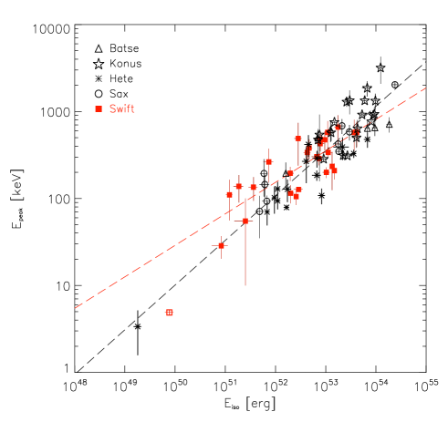
Figure 8: Rest frame $E_{\rm peak}-E_{\rm iso}$ correlation. The Swift bursts whose peak energy has been derived from the analysis of the BAT data are shown with filled red squares (their fit – excluding GRB 060218 – is represented by the solid red line). The non–Swift bursts are shown by the open symbols and their fit by the long–dashed black line.

In Fig. 8 we show in the $E_{\rm peak}-E_{\rm iso}$ plane, separately, the pre–Swift bursts and those whose spectral parameters have been determined only by Swift data. The best least square fit to the two sets of data yields a slope $a=0.51\pm 0.03$ for the pre–Swift GRBs and $a=0.36\pm 0.05$ for the Swift bursts. The two slopes become consistent if one performs a fit that weights for the errors on both quantities, as found by C07. However, for the Swift bursts of our sample, we have found the dominant selection effect. By accounting for this truncation we find a very weak correlation in the rest frame ($a=0.1$, Kendall’s $\tau=0.12$ at 0.58$\sigma$).

5 Summary and conclusions

In this paper we have studied the $E_{\rm peak}-E_{\rm iso}$ correlation defined with the most updated sample (up to Sep. 2007) of GRBs with measured redshift and well defined spectral properties: 35 GRBs detected before the launch of the Swift satellite (Nov. 2004) and 41 events detected since then. The latter sample is composed by 27 events whose spectral properties were obtained through the analysis of the Swift-BAT spectra and 14 bursts (in most cases also detected by Swift) but with a spectrum detected by other satellites (Konus, Suzaku, RHESSI) with a larger spectral energy window. With this large GRB sample we have studied the possible evolution with redshift, the existence of other correlations among the spectral parameters or with redshift, the possible instrumental selection effects acting on this sample of 76 GRBs with measured redshift.

Our main results show that in the rest frame $E_{\rm peak}-E_{\rm iso}$ plane the 76 GRBs define a strong correlation with no new outlier (with respect to the classical GRB 980425 and GRB 031203 (see e.g. Ghisellini et al. 2006). We find no correlation between the spectral parameters and the redshift nor between the peak energy and the spectral photon index.

By dividing the GRB sample into redshift bins we compared the slope of the $E_{\rm peak}$ correlation for each redshift bin. We do not find any evidence that this correlation evolves with redshift (as also found by B07) contrary to what has been found with a smaller GRB sample (Li 2007).

The analysis of the observer frame $E^{\rm obs}_{\rm peak}$–Fluence plane shows the existence of a strong correlation between the observed peak energy and the fluence. This correlation is of the form $E^{\rm obs}_{\rm peak}$$\propto$(Fluence)^0.4 and GRBs of different redshift are evenly distributed along it. The $E^{\rm obs}_{\rm peak}$–Fluence plane is where the possible selection effects on the $E_{\rm peak}$ correlation should be investigated. Two regions of this plane are defined by the $E^{\rm obs}_{\rm peak}$–Fluence correlation: bursts with large fluence and small/intermediate peak energy should not exist (or be very rare) as nothing prevents their detection, while bursts of intermediate/large $E^{\rm obs}_{\rm peak}$ and small fluence could be affected by some instrumental selection effect. We consider two of these: (a) the minimum flux to trigger a burst and (b) the minimum fluence required to fit its spectrum and constrain its peak energy. We have used the threshold curves derived by Band (2003) to represent the first selection effect in the $E^{\rm obs}_{\rm peak}$–Fluence plane. We have converted these curves into the fluence–$E^{\rm obs}_{\rm peak}$ plane, assuming a range of burst durations. We found that the trigger threshold does not affect the distribution of bursts with known redshifts in the $E^{\rm obs}_{\rm peak}$–Fluence plane. The second selection effect that we considered (to our knowledge this is the first time that such a selection effect is considered for the GRB detectors) is related to the requirement to have enough photons in the spectrum to fit it with a curved spectral model (either the Band model – Band et al. 1996 – or a cutoff–power law model) and constrain the peak energy of the burst. To this aim we performed detailed spectral simulations which account for the detector response and the typical GRB background. We also accounted for some parameters (burst duration and GRB off–axis position) which contribute to determine these threshold curves. Our results (shown in Fig. 5) demonstrate that the latter selection effect dominates the first in the $E^{\rm obs}_{\rm peak}$–Fluence plane as shown in Fig. 5. Our results show that the pre–Swift GRB sample, containing a fraction of bursts detected by BeppoSAX and BATSE  is not affected by the corresponding limiting curves, while the Swift sample is. Indeed, in the case of Swift most of the GRB whose spectra are well fitted by a cutoff–power law model have an $E^{\rm obs}_{\rm peak}$ which is in the range 15–150 keV. The correlation in the $E^{\rm obs}_{\rm peak}$–Fluence plane defined by the Swift sample is flat and very weak compared to that defined with all the other bursts. However, we cautiously note that the Swift sample is distributed in a very narrow range in $E^{\rm obs}_{\rm peak}$, smaller than the scatter of the $E^{\rm obs}_{\rm peak}$–Fluence correlation as defined by all the pre–Swift bursts. As a consequence, although Swift bursts do not show a $E^{\rm obs}_{\rm peak}$–Fluence correlation, we cannot rule out the existence of the very same correlation defined by the non–Swift bursts, extending over 2 orders of magnitudes in both $E^{\rm obs}_{\rm peak}$ and Fluence.

Our results do not exclude that other selection effects affect the $E^{\rm obs}_{\rm peak}$–Fluence plane, and in particular the non-Swift bursts. The lack of many bursts with known redshift with intermediate/large $E^{\rm obs}_{\rm peak}$and small fluence (i.e. between the present sample of GRBs and the BATSE limiting curves of Fig. 5) could be due to the additional presence of a still not understood selection effect, different from those considered in the present paper (see also Nakar & Piran 2005). The first step to investigate this possibility is to search if there exist GRBs which populate the region on the left side of the $E^{\rm obs}_{\rm peak}$–Fluence correlation. This issue cannot be solved by including, in the $E^{\rm obs}_{\rm peak}$–Fluence plot, the BATSE bursts already spectrally analyzed by Kaneko et al. (2006), since they all have large fluences. Furthermore, the sample of Yonetoku et al. (2004) could be biased by their requirement of having a pseudo–redshift not exceeding 12, as measured by the $E_{\rm peak}$–luminosity relation. Therefore we need a new, representative sample of BATSE bursts with measured $E^{\rm obs}_{\rm peak}$ and fluences close to the limiting fluence curve (see again Fig. 5). This is what we will present in a forthcoming paper (Nava et al. 2008, in preparation). We anticipate here that these bursts exist and therefore the conclusion that can be drawn from the present work is that other selection effects, different from the the GRB trigger threshold or the spectral threshold considered in the present paper, are very likely affecting the $E^{\rm obs}_{\rm peak}$–Fluence correlation and, as a consequence, the rest frame $E_{\rm peak}-E_{\rm iso}$ correlation.

References

- [] Amati, L., Frontera, F., Tavani, M., et al. 2002, A&A, 390, 81
- [] Amati, L., 2006, MNRAS, 372, 233
- [] Atteia J.-L., 2005, NCimC, 28, 647
- [] Band, D. L. et al., 1993, ApJ, 413, 281
- [] Band, D. L., 2003, ApJ, 588, 945
- [] Band, D. L., 2006, ApJ, 644, 378
- [] Band, D.L. & Preece, R.D., 2005, ApJ, 627, 319
- [] Bellm, E. C., Hurley, K., Palśhin, V., 2007, arXiv:0710.4590
- [] Blustin, A. J., Band, D., Barhelmy, S., 2006, ApJ, 637, 901
- [] Bosnjak, Z., Celotti, A., Longo, F., Barbiellini, G., 2007, MNRAS subm., astro-ph/0502185
- [] Butler, N.R., Kocevski, D., Bloom, J.S. & curtis, J.L., 2007, arXiv:0706.1275
- [] Cabrera, I., 2007, MNRAS, in press (C07), arXiv:0704.0791
- [] Campana, S., Mangano, V., Blustin, A. J., et al., 2006, Nat., 442, 1008
- [] Cenko, S. B., Kasliwal, M., Harrison, F. A., 2006, ApJ, 652, 490
- [] Crew G., Ricker, G., Atteia, J.-L., 2005, GCN 4021
- [] D’Agostini, G., 2005, arXiv:physics/0511182
- [] Eichler, D. & Levinson, A., 2004, ApJ, 614, L13
- [] Firmani C., Ghisellini, G., Avila-Reese, V. et al., 2006, MNRAS, 370, 185
- [] Frontera F., AIP conf proc. (astro-ph/ 0407633)
- [] Gehrels, N., Chincarini, G., Giommi P., et al., 2004, ApJ, 611, 1005
- [] Ghirlanda, G., Ghisellini, G. & Lazzati, D. 2004, ApJ, 616, 331
- [] Ghirlanda, G., Ghisellini, Firmani C., 2005, MNRAS, 361, 10L
- [] Ghirlanda, G, Nava, L., Ghisellini G., Firmani C., 2007, A&A, 466, 127
- [] Ghisellini, G., Ghirlanda, G., Mereghetti, S., Bosnjak, Z., Tavecchio, F., & Firmani, C., 2006, MNRAS, 372, 1699
- [] Golenetskii S., Aptekar R., Mazets E., et al., 2005, GCN 3179
- [] Golenetskii S., Aptekar R., Mazets E., et al., 2005a, GCN 3518
- [] Golenetskii S., Aptekar R., Mazets E., et al., 2005b, GCN 4328
- [] Golenetskii S., Aptekar R., Mazets E., et al., 2006, GCN 4989
- [] Golenetskii S., Aptekar R., Mazets E., et al., 2006a, GCN 5722
- [] Golenetskii S., Aptekar R., Mazets E., et al., 2006b, GCN 5837
- [] Golenetskii S., Aptekar R., Mazets E., et al., 2006c, GCN 4150
- [] Golenetskii S., Aptekar R., Mazets E., et al., 2006d, GCN 5460
- [] Golenetskii S., Aptekar R., Mazets E., et al., 2007, GCN 6049
- [] Guidorzi, C., Frontera, F., Montanari E., et al., 2005, MNRAS, 363, 315
- [] Kaneko, Y., Preece, R.D., Briggs, M.S., Paciesas, W.S., Meegan, C.A. & Band, L., 2006, ApJS, 166, 298 (K06)
- [] Lamb, D.Q., Donaghy, T.Q. & Graziani, C., 2005, ApJ, 620, 355
- [] Li, L.–X., 2007, MNRAS, 379, L55 (L07)
- [] Liang, E. & Zhang, B., 2005, ApJ, 633, L611
- [] Lloyd–Ronning, N. & Ramirez–Ruiz, E., 2002, ApJ, 576, 101L
- [] Lloyd–Ronning, N., Petrosian, V. & Mallozzi, R. S., 2000, ApJ, 534, 227 (LPM00)
- [] Mangano, V., Holland, S. T., Malesani, D., 2007, A&A, 470, 105
- [] Nakar, E. & Piran, T., 2005, MNRAS, 360, L73
- [] Nava, L., Ghisellini, G., Ghirlanda, G., Tavecchio, F. & Firmani, C. 2006, A&A, 450, 471
- [] Nava, L., Ghisellini, G., Ghirlanda, G., Cabrera, J.I., Firmani, C. & Avila-Reese, V., 2007, MNRAS, 377, 1464
- [] Norris, J. P., Marani, G. F., Bonnell, J. T., 2000, ApJ, 534, 248
- [] Norris, J. P., 2002, ApJ, 579, 386
- [] Palmer, D., Barbier, L., Barthelmy, S., 2006, GCN 4697
- [] Perri, M., Giommi, P., Capalbi M., et al., 2005, A&A, 442, L1
- [] Perley, D. A., Bloom, J. S., Butler, N. R., et al., 2007, ApJ, subm., astro-ph/0703538
- [] Preece, R. D., Briggs, M. S., Mallozzi, R. S., et al., 2000, ApJS, 126, 19
- [] Reichart D., Lamb D. Q., Fenimore E. E. et al., 2001, ApJ, 552, 57
- [] Reichart D., astro-ph/0508529
- [] Ramirez–Ruiz, E., Granot, J., Kouveliotou, C., Woosley, S.E., Patel, S.K. & Mazzali, P.A., 2005, ApJ, 625, L91
- [] Romano P., Campana, S., Chincarini, G., 2006, A&A, 456, 917
- [] Sakamoto, T., Nakagawa, Y., Torii, K., et al., 2004, AIPC, 727, 106
- [] Sakamoto, T., Lamb, D.Q., Kawai, N., et al., 2005, ApJ, 629, 311
- [] Sakamoto, T., Sato, G., Barbier, L., et al., 2006, HEAD Meeting Bullettin, 38, 380
- [] Sato, G., Yamazaki, R., Ioka, K., 2007, ApJ, 657, 359
- [] Schaefer, B. E., 2007, ApJ, 660, 16
- [] Stamatikos, M., Barbier, L., Barthelmy, S. D., 2006, GCN 5639
- [] Tagliaferri, G., Antonelli, L. A., Chincarini, G., et al., 2005, A&A, 443, L1
- [] Ulanov, M. V., Golenetskii, S. V., Frederiks, D. D., et al., 2005, NCimC, 20, 351
- [] Vetere, M.L., et al. 2007, A&A, 473, 347
- [] Willingale, R., O’Brien, P.T., Osborne, J.P., et al., 2007, ApJ, 662, 1093
- [] Yonetoku, D., Marakami, T., Nakamura, T., et al., 2004, ApJ, 609, 935