Generalized Navier Boundary Condition and Geometric Conservation Law for surface tension

Abstract

We consider two-fluid flow problems in an Arbitrary Lagrangian Eulerian (ALE) framework. The purpose of this work is twofold. First, we address the problem of the moving contact line, namely the line common to the two fluids and the wall. Second, we perform a stability analysis in the energy norm for various numerical schemes, taking into account the gravity and surface tension effects.

The problem of the moving contact line is treated with the so-called Generalized Navier Boundary Conditions. Owing to these boundary conditions, it is possible to circumvent the incompatibility between the classical no-slip boundary condition and the fact that the contact line of the interface on the wall is actually moving.

The energy stability analysis is based in particular on an extension of the Geometry Conservation Law (GCL) concept to the case of moving surfaces. This extension is useful to study the contribution of the surface tension.

The theoretical and computational results presented in this paper allow us to propose a strategy which offers a good compromise between efficiency, stability and artificial diffusion.

1 Introduction

A difficult problem in the modelling of two-fluid flows in a bounded domain concerns the displacement of the contact line, namely the points which are at the intersection of the solid boundary of the domain and the interface separating the two fluids. The difficulty comes from the fact that:

• the interface follows the fluid motion: the normal velocity of a point on the interface is the normal velocity of the fluid particle at the same point,

• the fluid particles near the boundary of the domain tend to have the same velocity as the points of the boundary.

Thus, if the velocity of the points on the boundary of the domain is zero (classical no-slip condition for a viscous fluid on a fixed wall), the moving contact line does not move: this is the so-called moving contact line problem. We refer to the review papers [20, 17] for an introduction to this problem.

We have to keep in mind that the no-slip boundary condition for viscous flows is only an approximation of the Navier boundary conditions (which relates the slip velocity relative to the wall to the shear rate boundary). The Navier boundary conditions has been assessed by molecular dynamics (MD) simulations, but fails in the vicinity of the contact line. One might think that continuum mechanics models (at the macroscopic level) are not able to represent the movement of the contact line. Nevertheless, hybrid experiments reported in [11, 12, 24] which consists in imposing the slip velocity obtained by MD simulation in a continuum model, have shown that continuum models may provide good results. Recently, Qian, Wang and Sheng [16, 17] have proposed a boundary conditions, the so-called Generalized Navier Boundary Condition (GNBC), which is completly defined at the continuum level and which seems to be in good agreement with MD results, including in the vicinity of the contact line. We also refer to [18] for a careful study using MD, also showing that continuum models can be used to described the dynamics of the contact line.

In [16, 17], this boundary condition is used with a finite difference scheme and the displacement of the interface between the two fluids is handled with a phase-field approach. In this paper, we show that the GNBC is very natural with a discretization method based on a variational formulation, like the finite element method. In addition, the ALE formulation we adopt is convenient to study the energy balance and it uses less numerical parameters than in a phase-field formulation (for which a free energy for the order parameter needs to be introduced, for example). The main drawback of the ALE method compared to other methods to follow a moving interface (like volume of fluid methods [13, 9], level set methods [22, 19] or phase-field formulation) is that it does not allow very large motion of the interface without remeshing, and it does not allow a change of topology of the domains occupied by each fluid. On the other hand, it is generally admitted that it is the method of choice when a precise computation of the position of the interface is required, with good robustness and conservation properties. The ALE formulation has been used in number of applications involving two-fluid flows. We refer for example to [7] for an application to the modelling of aluminium electrolysis cells, and to Section 6 for an application to flows in narrow channels.

For efficiency and simplicity, many numerical schemes for two-fluid flows decouple the fluid resolution and the movement of the interface. The interface displacement is therefore solved explicitly with respect to the computation of the fluid velocity and pressure. The variational formulation proposed in this study being well-suited to study the discrete energy of the system, we propose to quantify the spurious energy due the gravity and the surface tension when the interface displacement is handled explicitly. The Geometric Conservation Law (GCL) is a natural tool to perform this study. To analyse the contribution of the surface tension terms, we will have to extend the GCL to surface integral.

Here is the outline of the paper. In Section 2, the GNBC is introduced. The ALE formulation used to implement this boundary condition is detailed in Section 3. We prove some lemmata on Geometric Conservation Law in Section 4. We then study the energy conservation properties of the numerical scheme in Section 5. Finally, Section 6 is devoted to some numerical experiments which illustrate the theoretical results and investigate some alternative schemes.

2 The Generalized Navier Boundary Condition

We are interested in the two-fluid Navier-Stokes equations, posed on a bounded smooth domain $\Omega\subset\mathbb{R}^{d}$ (with $d=2$ or $d=3$), and the time interval $(0,T)$:

$$\left\{\begin{array}[]{l}\displaystyle{\frac{\partial(\rho{\boldsymbol{u}})}{\partial t}+{\rm div}(\rho{\boldsymbol{u}}\otimes{\boldsymbol{u}})-{\rm div}\left(\eta\left(\nabla{\boldsymbol{u}}+\nabla{\boldsymbol{u}}^{T}\right)\right)=-\nabla p+\gamma H{\boldsymbol{n}}_{\Sigma}\delta_{\Sigma}+\rho{\boldsymbol{g}}},\\ {\rm div}({\boldsymbol{u}})=0,\\ \displaystyle{\frac{\partial\rho}{\partial t}+{\rm div}(\rho{\boldsymbol{u}})=0}.\end{array}\right.$$ (1)

The equation is posed in the distributional sense. The velocity is denoted by ${\boldsymbol{u}}$, the density by $\rho$, the viscosity by $\eta$ and the pressure by $p$. The vector ${\boldsymbol{g}}$ denotes the gravity acceleration:

$${\boldsymbol{g}}=-g{\boldsymbol{e}}_{3}$$

where $({\boldsymbol{e}}_{1},{\boldsymbol{e}}_{2},{\boldsymbol{e}}_{3})$ is an orthonormal basis of the physical space. The term $\gamma H{\boldsymbol{n}}_{\Sigma}\delta_{\Sigma}$ is the surface tension term that we will describe in detail below. The system is complemented by initial conditions $({\boldsymbol{u}}(t=0),\rho(t=0))$. We suppose that $\rho(t=0)$ takes two different values $\rho_{1}$ and $\rho_{2}$. This property is then conserved as time evolves for the function $\rho$ so that each fluid is distinguished from the other by its density. In the following we denote by

$$\Omega_{i}(t)=\left\{{\boldsymbol{x}}\in\mathbb{R}^{d},\,\rho(t,{\boldsymbol{x}})=\rho_{i}\right\}$$ (2)

the domain occupied at time $t$ by the fluid $i$. We suppose that $\Omega_{i}(t)$ is a smooth domain, and we denote by

$$\Sigma(t)=\partial\Omega_{1}(t)\cap\partial\Omega_{2}(t)$$ (3)

the interface between the two liquids. The viscosity $\eta$ may depend on the fluid, so that $\eta=\eta(\rho)$ in (1). We denote in the following by

$${\boldsymbol{\sigma}}=\eta\left(\nabla{\boldsymbol{u}}+\nabla{\boldsymbol{u}}^{T}\right)$$ (4)

the viscous stress tensor. In the surface tension term $\gamma H{\boldsymbol{n}}_{\Sigma}\delta_{\Sigma}$, $\gamma$ is the surface tension coefficient between the two fluids (which is supposed to be constant in the following), ${\boldsymbol{n}}_{\Sigma}$ is the unit outward vector normal to $\Omega_{1}$ (see Figure 1) and $H$ is the mean curvature of the interface $\Sigma$ positively counted with respect to the normal ${\boldsymbol{n}}_{\Sigma}$. The distribution $\delta_{\Sigma}$ is defined by: for any smooth function $\psi$

$$\langle\delta_{\Sigma},\psi\rangle=\int_{\Sigma}\psi d\sigma_{\Sigma}$$ (5)

where $\sigma_{\Sigma}$ denotes the Lebesgue measure (i.e. the surface measure) on $\Sigma$.

Figure 1: The domain $\Omega$ and various unit vectors. The 2d picture (in the dotted line circle) represents the vectors contained in the plane orthogonal to ${\boldsymbol{t}}_{\partial\Sigma}$.

Let us now describe the boundary conditions. We first suppose the non-penetration condition:

$$({\boldsymbol{u}}-{\boldsymbol{u}}^{b})\cdot{\boldsymbol{n}}_{\partial\Omega}=0\text{ on $\partial\Omega$},$$ (6)

where ${\boldsymbol{n}}_{\partial\Omega}$ denotes the unit outward vector normal to $\Omega$ (see Figure 1) and ${\boldsymbol{u}}^{b}$ is the velocity of the boundary (${\boldsymbol{u}}-{\boldsymbol{u}}^{b}$ is the slip velocity, ${\boldsymbol{u}}^{b}=0$ for a fixed wall). In addition, we will suppose for the sake of simplicity that

$${\boldsymbol{u}}^{b}\cdot{\boldsymbol{n}}_{\partial\Omega}=0,$$

which implies that the the fluid lives in a fixed domain $\Omega$.

The fluid being viscous, we have to set another boundary condition on $\partial\Omega$. As explained in the introduction, the classical no-slip boundary condition (${\boldsymbol{u}}={\boldsymbol{u}}^{b}$ on $\partial\Omega$) would stick the interface on the wall, which is clearly unacceptable.

It may be worth recalling that the no-slip boundary condition is in fact an approximation of the Navier boundary condition:

$$\beta\left({\boldsymbol{u}}-{\boldsymbol{u}}^{b}\right)\cdot{\boldsymbol{\tau}}+{\boldsymbol{\sigma}}{\boldsymbol{n}}_{\partial\Omega}\cdot{\boldsymbol{\tau}}=0,$$ (7)

where $\beta$ is the slip coefficient. The coefficient $\beta$ is in practice very large, which explains that $({\boldsymbol{u}}-{\boldsymbol{u}}^{b}).{\boldsymbol{\tau}}=0$ is a good approximation in many cases.

As explained in the introduction, the Navier boundary condition is not appropriate to describe the moving contact line. This is the motivation of the Generalized Navier Boundary Conditions (GNBC) introduced in [16]. To state the GNBC, we need to define (see Figure 1) the following vectors, defined on the boundary $\partial\Sigma$ of the interface: ${\boldsymbol{t}}_{\partial\Sigma}={\boldsymbol{n}}_{\Sigma}\times{\boldsymbol{n}}_{\partial\Omega}$ the tangent vector to $\partial\Sigma$, ${\boldsymbol{m}}={\boldsymbol{t}}_{\partial\Sigma}\times{\boldsymbol{n}}_{\Sigma}$ and ${\boldsymbol{t}}_{\partial\Omega}={\boldsymbol{n}}_{\partial\Omega}\times{\boldsymbol{t}}_{\partial\Sigma}$. Both sets of vectors $({\boldsymbol{t}}_{\partial\Sigma},{\boldsymbol{n}}_{\Sigma},{\boldsymbol{m}})$ and $({\boldsymbol{t}}_{\partial\Sigma},{\boldsymbol{t}}_{\partial\Omega},{\boldsymbol{n}}_{\partial\Omega})$ are positively oriented orthonormal basis. The GNBC writes: for any vector ${\boldsymbol{\tau}}$ tangent to $\partial\Omega$,

$$\beta\left({\boldsymbol{u}}-{\boldsymbol{u}}^{b}\right)\cdot{\boldsymbol{\tau}}+{\boldsymbol{\sigma}}{\boldsymbol{n}}_{\partial\Omega}\cdot{\boldsymbol{\tau}}+\gamma\left({\boldsymbol{m}}\cdot{\boldsymbol{t}}_{\partial\Omega}-\cos(\theta_{s})\right){\boldsymbol{t}}_{\partial\Omega}\cdot{\boldsymbol{\tau}}\,\delta_{\partial\Sigma}=0,$$ (8)

where as above $\beta$ is the slip coefficient, $\gamma$ is the surface tension coefficient between the two fluids, and $\theta_{s}$ is the static contact angle at the solid surface. The distribution $\delta_{\partial\Sigma}$ is defined accordingly with (5) by: for any smooth function $\psi$

$$\langle\delta_{\partial\Sigma},\psi\rangle=\int_{\partial\Sigma}\psi dl_{\partial\Sigma}$$ (9)

where $l_{\partial\Sigma}$ denotes the Lebesgue measure (i.e. the length measure) on the curve $\partial\Sigma$.

Compared to the classical Navier boundary condition (7), we notice the extra term

$$\left({\boldsymbol{m}}\cdot{\boldsymbol{t}}_{\partial\Omega}-\cos(\theta_{s})\right),$$

which is called the uncompensated Young stress in [17]. This quantity measures the difference between the dynamic contact angle $\theta$ made by the interface $\Sigma$ and the boundary $\partial\Omega$ (we choose the convention that this angle is measured in the fluid $1$, see Figure 1) and the static contact angle $\theta_{s}$. In general, the definition of $\theta_{s}$ is a difficult problem both from the experimental and the theoretical standpoints. In our framework, $\theta_{s}$ is assumed to be a part of the data. The uncompensated Young stress is concentrated along the boundary of the interface and vanishes when the dynamic contact angle is equal to the static contact angle.

3 Variational formulation and discretization

The aim of this section is to derive a variational formulation of the system of equations (1), together with the boundary conditions (6)–(8).

3.1 The weak ALE formulation

We assume that for any time $t\geq 0$, there exists a smooth and bijective mapping $\hat{\mathcal{A}}_{t}$ from a reference domain $\hat{\Omega}$ (divided into two separate subdomains $\hat{\Omega}_{1}$ and $\hat{\Omega}_{2}$ such that $\overline{\hat{\Omega}}=\overline{\hat{\Omega}_{1}}\cup\overline{\hat{\Omega}_{2}}$) to the current domain $\Omega$ such that $\hat{\mathcal{A}}_{t}(\hat{\Omega}_{i})=\Omega_{i}(t)$ (see Figure 2). The inverse function (with respect to the space variable) of $\hat{\mathcal{A}}_{t}$ is denoted $\hat{\mathcal{A}}_{t}^{-1}$.

Figure 2: The partition of the domain $\Omega$ and the ALE mapping.

The velocity of the domain $\hat{\boldsymbol{w}}$ is defined by:

$$\hat{\boldsymbol{w}}(t,\hat{\boldsymbol{x}})=\frac{\partial}{\partial t}\hat{\mathcal{A}}_{t}(\hat{\boldsymbol{x}}).$$ (10)

For any function $\psi(t,.)$ defined on $\Omega$, we denote by $\hat{\psi}(t,.)$ the corresponding function defined on the reference domain $\hat{\Omega}$ by

$$\hat{\psi}(t,\hat{{\boldsymbol{x}}})=\psi(t,\hat{\mathcal{A}}_{t}(\hat{{\boldsymbol{x}}})).$$ (11)

For example, the velocity of the domain ${\boldsymbol{w}}$ on the current frame is defined by

$${\boldsymbol{w}}(t,{\boldsymbol{x}})=\hat{\boldsymbol{w}}(t,\hat{\mathcal{A}}_{t}^{-1}({\boldsymbol{x}})).$$ (12)

Notice that the functions $\psi$ and $\hat{\psi}$ are such that:

$$\frac{\partial\hat{\psi}}{\partial t}(t,\hat{{\boldsymbol{x}}})=\frac{\partial\psi}{\partial t}(t,\hat{\mathcal{A}}_{t}(\hat{{\boldsymbol{x}}}))+{\boldsymbol{w}}(t,\hat{\mathcal{A}}_{t}(\hat{{\boldsymbol{x}}}))\cdot\nabla\psi(t,\hat{\mathcal{A}}_{t}(\hat{{\boldsymbol{x}}})).$$ (13)

The fact that $\hat{\mathcal{A}}_{t}$ maps $\hat{\Omega}_{i}$ to $\Omega_{i}(t)$ ($i=1$ or $2$) implies that the velocity of the domain satisfies

$${\boldsymbol{w}}\cdot{\boldsymbol{n}}_{i}={\boldsymbol{u}}\cdot{\boldsymbol{n}}_{i}\mbox{ on $\partial\Omega_{i}$, }$$ (14)

where $i=1$ or $i=2$ and ${\boldsymbol{n}}_{i}$ denotes the unit outward vector normal to $\Omega_{i}$. The density $\rho$ of the fluid is such that:

$$\rho(t,{\boldsymbol{x}})=\hat{\rho}(\hat{\mathcal{A}}_{t}^{-1}({\boldsymbol{x}})),$$ (15)

where $\hat{\rho}$ is equal to $\rho_{1}$ on $\hat{\Omega}_{1}$ and $\rho_{2}$ on $\hat{\Omega}_{2}$.

The following functional spaces will be needed, respectively for the velocity ${\boldsymbol{u}}$ and the pressure $p$:

$$V=L^{2}(0,T;\mathbb{H}^{1}_{\boldsymbol{n}}(\Omega)),\quad M=L^{2}(0,T;L^{2}_{0}(\Omega)),$$

where

$$\mathbb{H}^{1}_{\boldsymbol{n}}(\Omega)=\left\{{\boldsymbol{u}}\in\left(H^{1}(\Omega)\right)^{d},{\boldsymbol{u}}\cdot{\boldsymbol{n}}_{\partial\Omega}=0\mbox{ on $\partial\Omega$}\right\},$$

and

$$L^{2}_{0}(\Omega)=\left\{p\in L^{2}(\Omega),\,\int_{\Omega}p=0\right\}.$$

We also introduce the test function spaces on the reference domain

$$\hat{V}=\mathbb{H}^{1}_{\boldsymbol{n}}(\hat{\Omega}),\qquad\hat{M}=L^{2}_{0}(\hat{\Omega}).$$

In the moving frame, the test function spaces are defined by

$$V_{T}=\{{\boldsymbol{v}}:[0,T]\times\Omega\rightarrow\mathbb{R}^{d},\,{\boldsymbol{v}}(t,{\boldsymbol{x}})=\hat{\boldsymbol{v}}(\hat{\mathcal{A}}_{t}^{-1}({\boldsymbol{x}})),\,\hat{\boldsymbol{v}}\in\hat{V}\},$$

$$M_{T}=\{q:[0,T]\times\Omega\rightarrow\mathbb{R},\,q(t,{\boldsymbol{x}})=\hat{q}(\hat{\mathcal{A}}_{t}^{-1}({\boldsymbol{x}})),\,\hat{q}\in\hat{M}\}.$$

Thus, the test functions do not depend on time in the reference frame $\hat{\Omega}$ whereas they do on the current one: more precisely, let ${\boldsymbol{v}}$ be in $V_{T}$, then for a fixed $\hat{\boldsymbol{x}}\in\hat{\Omega}$, ${\boldsymbol{v}}(t,\hat{\mathcal{A}}_{t}(\hat{\boldsymbol{x}}))$ does not depend on time while for a fixed ${\boldsymbol{x}}\in\Omega$, ${\boldsymbol{v}}(t,{\boldsymbol{x}})$ does.

We are now in position to state the weak ALE formulation. It is the following coupled problem: we look for a function $\hat{\mathcal{A}}_{t}:\hat{\Omega}\to\Omega$ and $({\boldsymbol{u}},p)$ in $V\times M$ such that ${\boldsymbol{u}}(t=0,.)={\boldsymbol{u}}_{0}$ and:

• The function $\hat{\mathcal{A}}_{t}$ is smooth and maps $\hat{\Omega}_{i}$ to $\Omega_{i}(t)$ ($i=1$ or $2$). The domains $\Omega_{i}(t)$ occupied by each fluid are thus defined by $\hat{\mathcal{A}}_{t}$ and the density of the fluid $\rho$ is defined by:

  $$\rho(t,{\boldsymbol{x}})=\hat{\rho}(\hat{\mathcal{A}}_{t}^{-1}({\boldsymbol{x}}))=\rho_{i},\qquad\mbox{ for }{\boldsymbol{x}}\in\Omega_{i}(t).$$ (16)

• For all $({\boldsymbol{v}},q)$ in $V_{T}\times M_{T}$,

  $$\left\{\begin{array}[]{l}\displaystyle{\frac{d}{dt}\int_{\Omega}\rho{\boldsymbol{u}}\cdot{\boldsymbol{v}}+\int_{\Omega}\rho({\boldsymbol{u}}-{\boldsymbol{w}})\cdot\nabla{\boldsymbol{u}}\cdot{\boldsymbol{v}}-\int_{\Omega}{\rm div}({\boldsymbol{w}})\rho{\boldsymbol{u}}\cdot{\boldsymbol{v}}}\\ \quad\displaystyle{+\int_{\Omega}\frac{\eta}{2}\left(\nabla{\boldsymbol{u}}+\nabla{\boldsymbol{u}}^{T}\right):\left(\nabla{\boldsymbol{v}}+\nabla{\boldsymbol{v}}^{T}\right)-\int_{\Omega}p\,{\rm div}({\boldsymbol{v}})}\\ \quad\displaystyle{=-\gamma\int_{\Sigma}\mathrm{tr}(\nabla_{\Sigma}{\boldsymbol{v}})\,d\sigma_{\Sigma}-\beta\int_{\partial\Omega}({\boldsymbol{u}}-{\boldsymbol{u}}^{b})\cdot{\boldsymbol{v}}}\\ \qquad\displaystyle{+\gamma\int_{\partial\Sigma}\cos(\theta_{s}){\boldsymbol{t}}_{\partial\Omega}\cdot{\boldsymbol{v}}\,dl_{\partial\Sigma}+\int_{\Omega}{\boldsymbol{f}}\cdot{\boldsymbol{v}},}\\ \displaystyle{\int_{\Omega}q\,{\rm div}({\boldsymbol{u}})=0.}\end{array}\right.$$ (17)

Of course, $\hat{\mathcal{A}}_{t}$ is not uniquely defined by the condition (16): this is the arbitrary feature of the ALE scheme. The function $\hat{\mathcal{A}}_{t}$ will be precisely defined at the discrete level in Section 3.3.3.

Notation: In (13), (17) and in the sequel, the spatial differential operators are taken with respect to the Eulerian variable ${\boldsymbol{x}}$. We omit to denote this explicitly for conciseness.

3.2 Derivation of the weak ALE formulation

Let us explain how this weak ALE formulation is obtained from the strong formulation (1), with the boundary conditions (6)–(8).

The starting point of this derivation is based on the following Lemma.

Lemma 1

For any smooth function $\psi$ depending on time $t$ and space ${\boldsymbol{x}}$, and any smooth function $\phi$ such that $\hat{\phi}$ (defined by $\hat{\phi}(t,\hat{{\boldsymbol{x}}})=\phi(t,\hat{\mathcal{A}}_{t}(\hat{{\boldsymbol{x}}}))$) is time-independent, we have:

$$\frac{d}{dt}\int_{\Omega}\psi(t,{\boldsymbol{x}})\,\phi(t,{\boldsymbol{x}})\,d{\boldsymbol{x}}$$

$$= \int_{\Omega}\phi(t,{\boldsymbol{x}})\frac{\partial\psi}{\partial t}(t,{\boldsymbol{x}})+\phi(t,{\boldsymbol{x}}){\boldsymbol{w}}(t,{\boldsymbol{x}})\cdot\nabla\psi(t,{\boldsymbol{x}})+\phi(t,{\boldsymbol{x}}){\rm div}({\boldsymbol{w}}(t,{\boldsymbol{x}}))\psi(t,{\boldsymbol{x}})\,d{\boldsymbol{x}}.$$

The first line in (17) is obtained by multiplying the material derivative in the equation on ${\boldsymbol{u}}$ in (1) by the test function ${\boldsymbol{v}}\in V_{T}$ and integrating over $\Omega$:

$$\int_{\Omega}\frac{\partial(\rho{\boldsymbol{u}})}{\partial t}\cdot{\boldsymbol{v}} +{\rm div}(\rho{\boldsymbol{u}}\otimes{\boldsymbol{u}})\cdot{\boldsymbol{v}}=\int_{\Omega}\rho\frac{\partial{\boldsymbol{u}}}{\partial t}\cdot{\boldsymbol{v}}+\rho{\boldsymbol{u}}\cdot\nabla{\boldsymbol{u}}\cdot{\boldsymbol{v}},$$

$$=\frac{d}{dt}\int_{\Omega}\rho{\boldsymbol{u}}\cdot{\boldsymbol{v}}-\int_{\Omega}\rho{\boldsymbol{w}}\cdot\nabla{\boldsymbol{u}}\cdot{\boldsymbol{v}}-{\rm div}({\boldsymbol{w}})\rho{\boldsymbol{u}}\cdot{\boldsymbol{v}}+\rho{\boldsymbol{u}}\cdot\nabla{\boldsymbol{u}}\cdot{\boldsymbol{v}},$$

where we used successively the equation on $\rho$ in (1) and then (1). The weak formulation of the terms involving the pressure are classically obtained by integration by parts. It is straightforward to obtain the following variational formulation for the term involving the viscous stress and the surface tension term:

$$\int_{\Omega}\frac{\eta}{2}\left(\nabla{\boldsymbol{u}}+\nabla{\boldsymbol{u}}^{T}\right):\left(\nabla{\boldsymbol{v}}+\nabla{\boldsymbol{v}}^{T}\right)-\int_{\partial\Omega}{\boldsymbol{\sigma}}{\boldsymbol{n}}_{\partial\Omega}\cdot{\boldsymbol{v}}-\int_{\Sigma}\gamma H{\boldsymbol{v}}\cdot{\boldsymbol{n}}_{\Sigma}d\sigma_{\Sigma}.$$ (19)

We now use the surface divergence formula (see [25] Equation (24) p. 239 or [1], Equation (3.8)). For any smooth hypersurface $\Sigma$ in $\mathbb{R}^{d}$ (i.e. a submanifold of $\mathbb{R}^{d}$ with codimension $1$) with a smooth boundary $\partial\Sigma$ and normal ${\boldsymbol{n}}_{\Sigma}({\boldsymbol{x}})$ at point ${\boldsymbol{x}}$, one has: for any smooth function ${\boldsymbol{\Phi}}:\Sigma\to\mathbb{R}^{d}$,

$$-\int_{\Sigma}H{\boldsymbol{\Phi}}\cdot{\boldsymbol{n}}_{\Sigma}\,d\sigma_{\Sigma}=\int_{\Sigma}\mathrm{tr}(\nabla_{\Sigma}{\boldsymbol{\Phi}})\,d\sigma_{\Sigma}-\int_{\partial\Sigma}{\boldsymbol{\Phi}}\cdot{\boldsymbol{m}}\,dl_{\partial\Sigma},$$ (20)

where the surface gradient $\nabla_{\Sigma}$ is defined by: for any smooth vector field ${\boldsymbol{X}}$,

$$\nabla_{\Sigma}{\boldsymbol{X}}=P_{\Sigma}({\boldsymbol{x}})\nabla{\boldsymbol{X}},$$ (21)

where $P_{\Sigma}({\boldsymbol{x}})$ is the orthogonal projector onto the tangent space to $\Sigma$ at point ${\boldsymbol{x}}$:

$$P_{\Sigma}({\boldsymbol{x}})=\rm Id-{\boldsymbol{n}}_{\Sigma}({\boldsymbol{x}})\otimes{\boldsymbol{n}}_{\Sigma}({\boldsymbol{x}}).$$

Notice that the surface gradient of ${\boldsymbol{X}}$ only depends on the values of ${\boldsymbol{X}}$ on the surface $\Sigma$. The vector ${\boldsymbol{m}}$ is the normal vector to $\partial\Sigma$ in the tangent space of $\Sigma$ pointing outwards of $\Sigma$ (see Figure 1). The measure $l_{\partial_{\Sigma}}$ is the Lebesgue measure on $\partial\Sigma$.

Using the surface divergence formula (20), the last two terms in (19) writes:

$$-\int_{\partial\Omega}{\boldsymbol{\sigma}}{\boldsymbol{n}}_{\partial\Omega}\cdot{\boldsymbol{v}}-\int_{\Sigma}\gamma H{\boldsymbol{v}}\cdot{\boldsymbol{n}}_{\Sigma}d\sigma_{\Sigma} =-\int_{\partial\Omega}{\boldsymbol{\sigma}}{\boldsymbol{n}}_{\partial\Omega}\cdot{\boldsymbol{v}}+\gamma\int_{\Sigma}\mathrm{tr}(\nabla_{\Sigma}{\boldsymbol{v}})\,d\sigma_{\Sigma}$$

$$\quad-\gamma\int_{\partial\Sigma}{\boldsymbol{v}}\cdot{\boldsymbol{m}}\,dl_{\partial\Sigma}.$$ (22)

We now use the GNBC (8) to rewrite the first and last terms in the right-hand side of (22):

$$- \int_{\partial\Omega}{\boldsymbol{\sigma}}{\boldsymbol{n}}_{\partial\Omega}\cdot{\boldsymbol{v}}-\gamma\int_{\partial\Sigma}{\boldsymbol{v}}\cdot{\boldsymbol{m}}\,dl_{\partial\Sigma}$$

$$=\beta\int_{\partial\Omega}({\boldsymbol{u}}-{\boldsymbol{u}}^{b})\cdot{\boldsymbol{v}}+\gamma\int_{\partial\Sigma}\left({\boldsymbol{m}}\cdot{\boldsymbol{t}}_{\partial\Omega}-\cos(\theta_{s})\right){\boldsymbol{t}}_{\partial\Omega}\cdot{\boldsymbol{v}}\,dl_{\partial\Sigma}-\gamma\int_{\partial\Sigma}{\boldsymbol{v}}\cdot{\boldsymbol{m}}\,dl_{\partial\Sigma},$$

$$=\beta\int_{\partial\Omega}({\boldsymbol{u}}-{\boldsymbol{u}}^{b})\cdot{\boldsymbol{v}}-\gamma\int_{\partial\Sigma}\cos(\theta_{s}){\boldsymbol{t}}_{\partial\Omega}\cdot{\boldsymbol{v}}\,dl_{\partial\Sigma},$$

where we have used the fact that ${\boldsymbol{v}}\cdot{\boldsymbol{m}}=\left({\boldsymbol{v}}\cdot{\boldsymbol{t}}_{\partial\Omega}\right)\left({\boldsymbol{m}}\cdot{\boldsymbol{t}}_{\partial\Omega}\right)$ (since ${\boldsymbol{v}}\cdot{\boldsymbol{n}}_{\partial\Omega}=0$).

With the divergence formula, we eliminate the mean curvature $H$ (which is difficult to approximate at the discrete level), and we naturally enforce the GNBC.

3.3 Discretization

The discretization is based on a finite element method in space, and an implicit Euler time-discretization. The domain $\overline{\Omega}^{n}=\overline{\Omega}^{n}_{1}\cup\overline{\Omega}^{n}_{2}$ at the beginning of the $n$-th timestep, where $\Omega^{n}_{i}$ is the domain occupied by the fluid $i$ at time $t_{n}$, plays the role of the reference domain $\overline{\hat{\Omega}}=\overline{\hat{\Omega}}_{1}\cup\overline{\hat{\Omega}}_{2}$.

Given the mesh ${\mathcal{M}}^{n}={\mathcal{M}}_{1}^{n}\cup{\mathcal{M}}_{2}^{n}$ of the domain $\overline{\Omega}^{n}=\overline{\Omega}_{1}^{n}\cup\overline{\Omega}_{2}^{n}$ and the velocity ${\boldsymbol{u}}^{n}$ discretized in a finite element space at time $t_{n}$, we aim to propagate these two items to time $t_{n+1}$, using the weak ALE formulation (17).

In addition to $({\mathcal{M}}^{n},{\boldsymbol{u}}^{n})$, let us give ourselves a space discretization of the domain velocity ${\boldsymbol{w}}^{n}$ at time $t_{n}$. Depending on the scheme (implicit or explicit treatment of the displacement of the domain) the velocity ${\boldsymbol{w}}^{n}$ may depend on ${\boldsymbol{u}}^{n}$ or on ${\boldsymbol{u}}^{n+1}$. We will come back to its computation below, in Section 3.3.3. We introduce the application

$${\mathcal{A}}_{n,n+1}:\left\{\begin{array}[]{ccc}(\Omega^{n}_{i})_{i=1,2}&\to&(\Omega^{n+1}_{i})_{i=1,2}\\ {\boldsymbol{y}}&\mapsto&{\boldsymbol{x}}={\boldsymbol{y}}+\delta t\,{\boldsymbol{w}}^{n}({\boldsymbol{y}})\end{array}\right.,$$ (23)

which might be seen as an approximation of $\hat{\mathcal{A}}_{t_{n+1}}\circ\hat{\mathcal{A}}_{t_{n}}^{-1}$. This application defines the domain occupied by each fluid at time $t_{n+1}$: $\Omega^{n+1}_{i}={\mathcal{A}}_{n,n+1}(\Omega^{n}_{i})$, for $i=1,2$. Without loss of generality, the time-step $\delta t=t_{n+1}-t_{n}$ is supposed to be constant. In the sequel, our convention is that ${\boldsymbol{y}}$ denotes a point in $(\Omega^{n}_{i})_{i=1,2}$ and ${\boldsymbol{x}}$ a point in $(\Omega^{n+1}_{i})_{i=1,2}$.

3.3.1 Discretization in space

We consider a finite element discretization of the domain $(\Omega^{n}_{i})_{i=1,2}$. It is transported by the application ${\mathcal{A}}_{n,n+1}$ to a finite element discretization of the domain $(\Omega^{n+1}_{i})_{i=1,2}$. The finite element spaces at time $t_{n}$ for the velocity and the pressure are respectively denoted by

$$V_{h,n}\subset\mathbb{H}^{1}_{\boldsymbol{n}}(\Omega),\qquad\qquad M_{h,n}\subset L^{2}_{0}(\Omega).$$

These finite element spaces depend on the time index $n$, since the mesh is moving. They are supposed to satisfy the inf-sup condition (see [4, 8] for example).

As explained above, we use test functions which follow the deformation of the domain given by ${\mathcal{A}}_{n,n+1}$: the test functions at time $t_{n+1}$ belong to the following spaces:

$$V_{h,n+1}=\{{\boldsymbol{v}}(t_{n+1},.):\Omega\rightarrow\mathbb{R}^{N},{\boldsymbol{v}}(t_{n+1},{\boldsymbol{x}})={\boldsymbol{v}}(t_{n},{\mathcal{A}}_{n,n+1}^{-1}({\boldsymbol{x}})),{\boldsymbol{v}}(t_{n},.)\in V_{h,n}\},$$

$$M_{h,n+1}=\{q(t_{n+1},.):\Omega\rightarrow\mathbb{R},q(t_{n+1},{\boldsymbol{x}})=q(t_{n},{\mathcal{A}}_{n,n+1}^{-1}({\boldsymbol{x}})),q(t_{n},.)\in M_{h,n}\}.$$

Unless there is a risk of confusion, we omit the index $h$ for the functions belonging to the finite element spaces $V_{h,n}$ or $M_{h,n}$.

3.3.2 Time discretization and linearization

We use the following semi-implicit Euler discretization of (17): for a given ${\boldsymbol{u}}^{n}\in V_{h,n}$, $(\Omega^{n}_{i})_{i=1,2}$, ${\boldsymbol{w}}^{n}$ and $(\Omega^{n+1}_{i})_{i=1,2}$, compute $({\boldsymbol{u}}^{n+1},p^{n+1})\in V_{h,n+1}\times M_{h,n+1}$ such that, for all $({\boldsymbol{v}}(t_{n},.),q(t_{n},.))\in V_{h,n}\times M_{h,n}$,

$$\left\{\begin{array}[]{l}\displaystyle{\frac{1}{\delta t}\int_{\Omega^{n+1}}\rho{\boldsymbol{u}}^{n+1}\cdot{\boldsymbol{v}}+\int_{\Omega^{n+1}}\rho({\boldsymbol{u}}^{n}-{\boldsymbol{w}}^{n})\cdot\nabla{\boldsymbol{u}}^{n+1}\cdot{\boldsymbol{v}}-\int_{\Omega^{n+1}}{\rm div}({\boldsymbol{w}}^{n})\rho{\boldsymbol{u}}^{n+1}\cdot{\boldsymbol{v}}}\\ \displaystyle{\quad+\int_{\Omega^{n+1}}\frac{\eta}{2}(\nabla{\boldsymbol{u}}^{n+1}+(\nabla{\boldsymbol{u}}^{n+1})^{T}):(\nabla{\boldsymbol{v}}+\nabla{\boldsymbol{v}}^{T})-\int_{\Omega^{n+1}}p^{n+1}{\rm div}({\boldsymbol{v}})}\\ \displaystyle{\quad+\int_{\Omega^{n+1}}\frac{\rho}{2}\,{\rm div}({\boldsymbol{u}}^{n})\,{\boldsymbol{u}}^{n+1}\cdot{\boldsymbol{v}}+\frac{\delta\rho}{2}\int_{\Sigma^{n+1}}({\boldsymbol{u}}^{n}-{\boldsymbol{w}}^{n})\cdot{\boldsymbol{n}}_{\Sigma^{n+1}}\,{\boldsymbol{u}}^{n+1}\cdot{\boldsymbol{v}}\,d\sigma_{\Sigma^{n+1}}}\\ \displaystyle{\qquad=\frac{1}{\delta t}\int_{\Omega^{n}}\rho{\boldsymbol{u}}^{n}\cdot{\boldsymbol{v}}-\gamma\int_{\Sigma^{n+1}}\mathrm{tr}(\nabla_{\Sigma^{n+1}}{\boldsymbol{v}})d\sigma_{\Sigma^{n+1}}-\beta\int_{\partial\Omega^{n+1}}({\boldsymbol{u}}^{n+1}-{\boldsymbol{u}}^{b})\cdot{\boldsymbol{v}}}\\ \displaystyle{\qquad\quad+\gamma\int_{\partial\Sigma^{n+1}}\cos(\theta_{s}){\boldsymbol{t}}_{\partial\Omega}\cdot{\boldsymbol{v}}\,dl_{\partial\Sigma^{n+1}}+\int_{\Omega^{\star}}\rho{\boldsymbol{g}}\cdot{\boldsymbol{v}},}\\ \displaystyle{\int_{\Omega^{n+1}}q{\rm div}({\boldsymbol{u}}^{n+1})=0.}\end{array}\right.$$ (24)

Notice that the superscript $n$ (in $\Omega^{n}$) emphasizes that we consider the domain at time $t^{n}$, even if the boundary of the domain is not moving. When we integrate over $\Omega^{n+1}$, this is to indicate that the test functions and the functions $\rho$, $\eta$ (whose values are deduced from the domains occupied by each fluid) are taken at time $t_{n+1}$. If a function defined on $\Omega^{n}$ appears in an integral over $\Omega^{n+1}$, it means that this function is transported on $\Omega^{n+1}$ by ${\mathcal{A}}_{n,n+1}$. For example,

$$\int_{\Omega^{n+1}}\frac{\rho}{2}\,{\rm div}({\boldsymbol{u}}^{n})\,{\boldsymbol{u}}^{n+1}\cdot{\boldsymbol{v}}=\sum_{i=1}^{2}\frac{\rho_{i}}{2}\int_{\Omega_{i}^{n+1}}{\rm div}({\boldsymbol{u}}^{n}\circ{\mathcal{A}}_{n,n+1}^{-1})\,{\boldsymbol{u}}^{n+1}\cdot{\boldsymbol{v}}(t_{n+1},.).$$

The discretization (24) is obtained from the weak ALE formulation (17). In the third line of (24) appear two terms which are required for better stability properties of the scheme. The term $\displaystyle{\int_{\Omega^{n+1}}\frac{\rho}{2}\,{\rm div}({\boldsymbol{u}}^{n})\,{\boldsymbol{u}}^{n+1}\cdot{\boldsymbol{v}}}$ is standard. It is analogous to the well-known modification introduced by Temam of the convective term (see Section III.5 in [23]) which allows to recover at the discrete level the skew-symmetry property of the advection term. The second term $\displaystyle{\frac{\delta\rho}{2}\int_{\Sigma^{n+1}}({\boldsymbol{u}}^{n}-{\boldsymbol{w}}^{n})\cdot{\boldsymbol{n}}_{\Sigma}\,{\boldsymbol{u}}^{n+1}\cdot{\boldsymbol{v}}\,d\sigma}$ where we have used the notation

$$\delta\rho=\rho_{2}-\rho_{1},$$ (25)

is in the same vein, but is specific to the context of two-fluid flows. Notice that both these terms are strongly consistent: they vanish for the exact solution. They are introduced in order to reproduce at the discrete level the energy estimates that can be derived at the continuous level (see Section 5).

The body force is integrated on a domain denoted by $\Omega^{\star}$. We will consider in the sequel different choices: $\Omega^{\star}=\Omega^{n}$ or $\Omega^{n+1}$ or $\Omega^{n+1/2}$. By convention, we define the quantity $\int_{\Omega^{n+1/2}}\rho{\boldsymbol{g}}\cdot{\boldsymbol{v}}$ as

$$\int_{\Omega^{n+1/2}}\rho{\boldsymbol{g}}\cdot{\boldsymbol{v}}=\frac{1}{2}\int_{\Omega^{n+1}}\rho{\boldsymbol{g}}\cdot{\boldsymbol{v}}+\frac{1}{2}\int_{\Omega^{n}}\rho{\boldsymbol{g}}\cdot{\boldsymbol{v}}.$$

It is worth noticing that the three choices have the same computational cost as soon as the mesh velocity ${\boldsymbol{w}}^{n}$ is explicitly obtained from the known velocity ${\boldsymbol{u}}^{n}$.They nevertheless lead to very different behaviors, as shown in Section 6.1.

3.3.3 The complete algorithm

To complete the presentation of the numerical scheme, it remains to describe how the domain velocity ${\boldsymbol{w}}^{n}$ is computed. The basic requirement is the kinematic condition (14), which ensures in particular that the nodes of the mesh which are initially on the interface remain on the interface. In addition, ${\mathcal{A}}_{n,n+1}$ defined from ${\boldsymbol{w}}^{n}$ by (23) must be sufficiently smooth so that the mesh remains regular enough for finite element computations.

In the practical problems we are interested in, it is sufficient to adopt the very standard method that consists in solving a simple Poisson problem to compute the velocity of the mesh. Moreover, we choose the displacement to be along one direction only, so that we actually solve a scalar Poisson problem. This choice, which is definitely reasonable in the physical situations that we consider, has important favorable consequences on the quality of the algorithm. This will be made precise in Section 5.2. In addition, we discretize the velocity of the domain ${\boldsymbol{w}}^{n}$ in space using the same finite element space as for the components of ${\boldsymbol{u}}^{n}$.

We may now write the complete algorithm. Suppose that $(\Omega^{n}_{i})_{i=1,2}$ and $({\boldsymbol{u}}^{n},p^{n})$ are known. Then ${\boldsymbol{w}}^{n}$, $(\Omega^{n+1}_{i})_{i=1,2}$ and $({\boldsymbol{u}}^{n+1},p^{n+1})$ are computed as follows:

• Compute the terms defined on $\Omega^{n}$ $\bigg{(}$like $\displaystyle{\frac{1}{\delta t}\int_{\Omega^{n}}\rho{\boldsymbol{u}}^{n}\cdot{\boldsymbol{v}}\,d{\boldsymbol{x}}}$$\bigg{)}$ in the system (24).

• Compute ${\boldsymbol{w}}^{n}=(0,0,w^{n})$. We consider two options:

  • Scheme (M1) : explicit treatment of the displacement of the interface

    $$\left\{\begin{array}[]{rcll}-\Delta w^{n}&=&0,&\mbox{ on }\Omega_{i}^{n},i=1,2,\\ w^{n}&=&\displaystyle{\frac{{\boldsymbol{u}}^{n}\cdot{\boldsymbol{n}}_{\Sigma^{n}}}{n_{\Sigma^{n}}^{3}}},&\mbox{ on }\Sigma^{n},\\ \displaystyle{\frac{\partial w^{n}}{\partial{\boldsymbol{n}}}}&=&0,&\mbox{ on }\partial\Omega,\end{array}\right.$$ (26)

  • Scheme (M2) : implicit treatment of the displacement of the interface

    $$\left\{\begin{array}[]{rcll}-\Delta w^{n}&=&0,&\mbox{ on }\Omega_{i}^{n+1},i=1,2,\\ w^{n}\circ{\mathcal{A}}_{n,n+1}^{-1}&=&\displaystyle{\frac{{\boldsymbol{u}}^{n+1}\cdot{\boldsymbol{n}}_{\Sigma^{n+1}}}{n_{\Sigma^{n+1}}^{3}}},&\mbox{ on }\Sigma^{n+1},\\ \displaystyle{\frac{\partial w^{n}}{\partial{\boldsymbol{n}}}}&=&0,&\mbox{ on }\partial\Omega.\end{array}\right.$$ (27)

  where the components of the normal ${\boldsymbol{n}}_{\Sigma}$ are denoted by $(n_{\Sigma}^{1},n_{\Sigma}^{2},n_{\Sigma}^{3})$.

• Move the nodes of the mesh according to ${\mathcal{A}}_{n,n+1}$ defined by (23).

• Compute the remaining terms (defined on $\Omega^{n+1}$) in the system (24).

• Solve (24) to determine $({\boldsymbol{u}}^{n+1},p^{n+1})$. The resolution is typically performed by a GMRES iterative procedure with an ILU preconditioner and $({\boldsymbol{u}}^{n},p^{n})$ as the initial guess.

In step (ii), the implementation of the Dirichlet boundary condition on $w$ is made easier by defining the normals ${\boldsymbol{n}}_{\Sigma}$ at each node of the discretized surface $\Sigma^{n}$. Such a definition is delicate, since $\Sigma^{n}$ is only piecewise smooth, and the nodes are typically singular points of $\Sigma^{n}$. In practice, following [3], we use approximated normals ${\boldsymbol{n}}_{\Sigma,h}$ at each node of the interface, by requiring that the Stokes integration by parts formula holds at the discrete level. This is one of the ingredient which ensures the exact mass conservation of each fluids on the discretized system. We refer to Section 5.1.3.2 in [7] or to [6] for more details.

Note that scheme (M2) is much more expensive than scheme (M1) since it requires the resolution of a nonlinear system (the velocity ${\boldsymbol{u}}^{n+1}$ and the domains $\Omega^{n+1}_{i}$ being unknown when ${\boldsymbol{w}}^{n}$ is computed). The resulting nonlinear system can be typically solved with a Newton algorithm (see for example [21]). For this study, we chose a relaxed fixed-point method, solving iteratively systems (24) and (27) at each time step.

4 Surface Geometric Conservation Law

We establish in this section a few technical results that will be useful to study the discrete energy of the system.

Let $\phi$ be a test function such that $\hat{\phi}$ (defined by $\hat{\phi}(t,\hat{{\boldsymbol{x}}})=\phi(t,\hat{\mathcal{A}}_{t}(\hat{{\boldsymbol{x}}}))$) is time-independent. Taking $\psi=1$ in (1), we readily have

$$\frac{d}{dt}\int_{\Omega}\phi(t,{\boldsymbol{x}})\,d{\boldsymbol{x}}=\int_{\Omega}\phi(t,{\boldsymbol{x}})\,{\rm div}{\boldsymbol{w}}(t,{\boldsymbol{x}})\,d{\boldsymbol{x}},$$ (28)

There is an analogous formula to compute the time derivative of the surface integral of $\phi$ (see [2], formula (4.17) p. 355):

$$\frac{d}{dt}\int_{\Sigma_{t}}\phi(t,.)\,d\sigma_{\Sigma_{t}}=\int_{\Sigma_{t}}\phi\,\mathrm{tr}(\nabla_{\Sigma_{t}}({\boldsymbol{w}}))\,d\sigma_{\Sigma_{t}}.$$ (29)

The so-called Geometric Conservation Law (GCL) is related to equation (28). The precise definition of GCL may differ from an author to another (see e.g. [15, 14, 10, 5]). Here we will say that the GCL is satisfied when the equality in (28) is preserved after time discretization. The following lemma states that the GCL is satisfied as soon as the mesh velocity has only one nonvanishing component.

Lemma 2 (GCL)

Suppose that the domain velocity ${\boldsymbol{w}}^{n}$ has the form $(0,0,w^{n})$. Let $\phi$ be a function defined on $\Omega_{i}^{n+1}$, for $i=1$ or $2$. Then the ALE scheme satisfies the GCL in the following sense:

$$\int_{\Omega_{i}^{n+1}}\!\!\!\!\!\phi({\boldsymbol{x}})\,d{\boldsymbol{x}}-\int_{\Omega_{i}^{n}}\!\!\!\phi\circ{\mathcal{A}}_{n,n+1}({\boldsymbol{y}})\,d{\boldsymbol{y}}$$ (30)

$$= \delta t\int_{\Omega_{i}^{n}}\!\!\!\phi\circ{\mathcal{A}}_{n,n+1}({\boldsymbol{y}}){\rm div}_{\boldsymbol{y}}{\boldsymbol{w}}^{n}({\boldsymbol{y}})\,d{\boldsymbol{y}},$$

$$= \delta t\int_{\Omega_{i}^{n+1}}\!\!\!\!\!\phi({\boldsymbol{x}}){\rm div}_{\boldsymbol{x}}\left({\boldsymbol{w}}^{n}\circ{\mathcal{A}}_{n,n+1}^{-1}({\boldsymbol{x}})\right)\,d{\boldsymbol{x}}.$$ (31)

We refer to [6] or to [7] for the proof of this result. Formulas (30) and (31) are useful to establish the following lemma which will be used to study the effect of the gravity on the energy balance.

Lemma 3

Under the assumption of Lemma 2, we have:

$$\int_{\Sigma^{n}}gx_{3}\,\delta\rho\,{\boldsymbol{w}}^{n}\cdot{\boldsymbol{n}}_{\Sigma^{n}} =\int_{\Sigma^{n}}gx_{3}\,\delta\rho\,w^{n}n^{3}_{\Sigma^{n}},$$

$$=-\frac{1}{\delta t}\left(\int_{\Omega^{n+1}}\rho gx_{3}d{\boldsymbol{x}}-\int_{\Omega^{n}}\rho gx_{3}d{\boldsymbol{x}}\right)-\frac{\delta t}{2}\int_{\Sigma^{n}}\delta\rho g(w^{n})^{2}n^{3}_{\Sigma^{n}},$$ (32)

and

$$\int_{\Sigma^{n+1}}gx_{3}\,\delta\rho\, {\boldsymbol{w}}^{n}\circ{\mathcal{A}}_{n,n+1}^{-1}\cdot{\boldsymbol{n}}_{\Sigma^{n+1}}=\int_{\Sigma^{n+1}}gx_{3}\,\delta\rho\,w^{n}\circ{\mathcal{A}}_{n,n+1}^{-1}n^{3}_{\Sigma^{n+1}},$$

$$=-\frac{1}{\delta t}\left(\int_{\Omega^{n+1}}\rho gx_{3}d{\boldsymbol{x}}-\int_{\Omega^{n}}\rho gx_{3}d{\boldsymbol{x}}\right)+\frac{\delta t}{2}\int_{\Sigma^{n}}\delta\rho g(w^{n})^{2}n^{3}_{\Sigma^{n}}.$$ (33)

Proof. Formula (30) applied to the function $\rho gx_{3}$ yields

$$\int_{\Omega^{n+1}}\rho gx_{3} =\int_{\Omega^{n}}\rho g(y_{3}+\delta tw^{n}({\boldsymbol{y}}))\,d{\boldsymbol{y}}+\delta t\int_{\Omega^{n}}\rho g(y_{3}+\delta tw^{n}({\boldsymbol{y}}))\partial_{y_{3}}w^{n}\,d{\boldsymbol{y}},$$

$$=\int_{\Omega^{n}}\rho gy_{3}+\delta t\left(\int_{\Omega^{n}}\rho gw^{n}({\boldsymbol{y}})\,d{\boldsymbol{y}}+\int_{\Omega^{n}}\rho gy_{3}\partial_{y_{3}}w^{n}\,d{\boldsymbol{y}}\right)+\delta t^{2}\int_{\Omega^{n}}\rho gw^{n}\partial_{y_{3}}w^{n}\,d{\boldsymbol{y}},$$

$$=\int_{\Omega^{n}}\rho gy_{3}+\delta t\int_{\Omega^{n}}\rho g\partial_{y_{3}}(y_{3}w^{n})\,d{\boldsymbol{y}}+\frac{\delta t^{2}}{2}\int_{\Omega^{n}}\rho g\partial_{y_{3}}((w^{n})^{2})\,d{\boldsymbol{y}},$$

$$=\int_{\Omega^{n}}\rho gy_{3}-\delta t\int_{\Sigma^{n}}\delta\rho gy_{3}w^{n}n^{3}_{\Sigma^{n}}-\frac{\delta t^{2}}{2}\int_{\Sigma^{n}}\delta\rho g(w^{n})^{2}n^{3}_{\Sigma^{n}},$$

from which we deduce (32). We recall that $\delta\rho$ is defined by (25). For the second formula, we use (31):

$$\int_{\Omega^{n+1}}\rho gx_{3} =\int_{\Omega^{n}}\rho g(y_{3}+\delta tw^{n}({\boldsymbol{y}}))\,d{\boldsymbol{y}}+\delta t\int_{\Omega^{n+1}}\rho gx_{3}\partial_{x_{3}}\left(w^{n}\circ{\mathcal{A}}_{n,n+1}^{-1}({\boldsymbol{x}})\right)\,d{\boldsymbol{x}},$$

$$=\int_{\Omega^{n}}\rho g(y_{3}+\delta tw^{n}({\boldsymbol{y}}))\,d{\boldsymbol{y}}-\delta t\int_{\Omega^{n+1}}\partial_{x_{3}}\left(\rho gx_{3}\right)w^{n}\circ{\mathcal{A}}_{n,n+1}^{-1}({\boldsymbol{x}})\,d{\boldsymbol{x}},$$

$$=\int_{\Omega^{n}}\rho g(y_{3}+\delta tw^{n}({\boldsymbol{y}}))\,d{\boldsymbol{y}}-\delta t\int_{\Omega^{n+1}}\rho gw^{n}\circ{\mathcal{A}}_{n,n+1}^{-1}({\boldsymbol{x}})\,d{\boldsymbol{x}}$$

$$\quad-\delta t\int_{\Sigma^{n+1}}\delta\rho gx_{3}n^{3}_{\Sigma^{n+1}}w^{n}\circ{\mathcal{A}}_{n,n+1}^{-1},$$

$$=\int_{\Omega^{n}}\rho gy_{3}+\delta t\left(\int_{\Omega^{n}}\rho gw^{n}({\boldsymbol{y}}))\,d{\boldsymbol{y}}-\int_{\Omega^{n+1}}\rho gw^{n}\circ{\mathcal{A}}_{n,n+1}^{-1}({\boldsymbol{x}})\,d{\boldsymbol{x}}\right)$$

$$\quad-\delta t\int_{\Sigma^{n+1}}\delta\rho gx_{3}n^{3}_{\Sigma^{n+1}}w^{n}\circ{\mathcal{A}}_{n,n+1}^{-1},$$

$$=\int_{\Omega^{n}}\rho gy_{3}-\delta t^{2}\left(\int_{\Omega^{n}}\rho gw^{n}\partial_{y_{3}}w^{n}\,d{\boldsymbol{y}}\right)-\delta t\int_{\Sigma^{n+1}}\delta\rho gx_{3}n^{3}_{\Sigma^{n+1}}w^{n}\circ{\mathcal{A}}_{n,n+1}^{-1},$$

$$=\int_{\Omega^{n}}\rho gy_{3}-\delta t\int_{\Sigma^{n+1}}\delta\rho gx_{3}n^{3}_{\Sigma^{n+1}}w^{n}\circ{\mathcal{A}}_{n,n+1}^{-1}-\frac{\delta t^{2}}{2}\left(\int_{\Omega^{n}}\rho g\partial_{y_{3}}(w^{n})^{2}\right),$$

$$=\int_{\Omega^{n}}\rho gy_{3}-\delta t\int_{\Sigma^{n+1}}\delta\rho gx_{3}n^{3}_{\Sigma^{n+1}}w^{n}\circ{\mathcal{A}}_{n,n+1}^{-1}+\frac{\delta t^{2}}{2}\left(\int_{\Sigma^{n}}\delta\rho\,g(w^{n})^{2}n^{3}_{\Sigma^{n}}\right),$$

which gives (33). $\diamondsuit$

The above results are useful to study the energy balance at the discrete level in the presence of gravity. To study the effect of surface tension on the energy balance, we have to introduce a notion of ”Surface GCL”, namely we have to check how equality (29) is preserved by the time scheme. Contrarily to the volume case, we are not able to prove that the scheme satisfies a ”Surface GCL”. Nevertheless, we can establish inequalities which will be convenient in the sequel.

Lemma 4 (Surface GCL)

Suppose that the domain velocity ${\boldsymbol{w}}^{n}$ has the form $(0,0,w^{n})$. Let $\phi$ be a function defined on $\Sigma^{n+1}$. Then, if $\delta t$ is sufficiently small so that

$$1+\delta t\,\mathrm{tr}\left(\nabla_{\Sigma^{n}}\left({\boldsymbol{w}}^{n}\right)\right)\geq 0\qquad\text{on $\Sigma^{n}$},$$ (34)

the ALE scheme is such that:

$$\int_{\Sigma^{n+1}}\phi\,d\sigma_{\Sigma^{n+1}}-\int_{\Sigma^{n}}\phi\circ{\mathcal{A}}_{n,n+1}\,d\sigma_{\Sigma^{n}}\geq\delta t\int_{\Sigma^{n}}\phi\circ{\mathcal{A}}_{n,n+1}\mathrm{tr}(\nabla_{\Sigma^{n}}({\boldsymbol{w}}^{n}))\,d\sigma_{\Sigma^{n}}.$$ (35)

Likewise, if $\delta t$ is sufficiently small so that

$$1-\delta t\,\mathrm{tr}\left(\nabla_{\Sigma^{n+1}}\left({\boldsymbol{w}}^{n}\circ{\mathcal{A}}_{n,n+1}^{-1}\right)\right)\geq 0\qquad\text{on $\Sigma^{n+1}$},$$ (36)

the ALE scheme is such that:

$$\int_{\Sigma^{n+1}}\phi\,d\sigma_{\Sigma^{n+1}}-\int_{\Sigma^{n}}\phi\circ{\mathcal{A}}_{n,n+1}\,d\sigma_{\Sigma^{n}}\leq\delta t\int_{\Sigma^{n+1}}\phi\,\mathrm{tr}(\nabla_{\Sigma^{n+1}}({\boldsymbol{w}}^{n}\circ{\mathcal{A}}_{n,n+1}^{-1}))\,d\sigma_{\Sigma^{n+1}}.$$ (37)

Moreover, in both cases, the difference between the two sides of the inequalities (35) and (37) is of order $\delta t^{2}$ in the limit $\delta t\to 0$.

Proof. We only consider (35), the proof of (37) being similar. By a change of variable we have (see [2, Formula (4.9) p. 353]):

$$\int_{\Sigma^{n+1}}\phi d\sigma_{\Sigma^{n+1}} =\int_{\Sigma^{n}}\phi\circ{\mathcal{A}}_{n,n+1}\left|{\rm Cof}(\nabla{\mathcal{A}}_{n,n+1}){\boldsymbol{n}}_{\Sigma^{n}}\right|d\sigma_{\Sigma^{n}},$$

$$=\int_{\Sigma^{n}}\phi\circ{\mathcal{A}}_{n,n+1}\left|{\boldsymbol{n}}_{\Sigma^{n}}+\delta t\left(\begin{array}[]{c}n^{1}_{\Sigma^{n}}\partial_{y_{3}}w^{n}-n^{3}_{\Sigma^{n}}\partial_{y_{1}}w^{n}\\ n^{2}_{\Sigma^{n}}\partial_{y_{3}}w^{n}-n^{3}_{\Sigma^{n}}\partial_{y_{2}}w^{n}\\ 0\end{array}\right)\right|d\sigma_{\Sigma^{n}},$$

where ${\rm Cof}(\nabla{\mathcal{A}}_{n,n+1})$ denotes the matrix of cofactors of the Jacobian $\nabla{\mathcal{A}}_{n,n+1}$.

Let us consider the difference

$$\left|{\boldsymbol{n}}_{\Sigma^{n}}+\delta t\left(\begin{array}[]{c}n^{1}_{\Sigma^{n}}\partial_{y_{3}}w^{n}-n^{3}_{\Sigma^{n}}\partial_{y_{1}}w^{n}\\ n^{2}_{\Sigma^{n}}\partial_{y_{3}}w^{n}-n^{3}_{\Sigma^{n}}\partial_{y_{2}}w^{n}\\ 0\end{array}\right)\right|^{2}-\left|1+\delta t\,\mathrm{tr}\left(\nabla_{\Sigma^{n}}\left({\boldsymbol{w}}^{n}\right)\right)\right|^{2}.$$ (38)

The first term writes:

$$1+2\delta t\left((n^{1}_{\Sigma^{n}})^{2}\partial_{y_{3}}w^{n}-n^{1}_{\Sigma^{n}}n^{3}_{\Sigma^{n}}\partial_{y_{1}}w^{n}+(n^{2}_{\Sigma^{n}})^{2}\partial_{y_{3}}w^{n}-n^{2}_{\Sigma^{n}}n^{3}_{\Sigma^{n}}\partial_{y_{2}}w^{n}\right)$$

$$+\delta t^{2}\left(\left(n^{1}_{\Sigma^{n}}\partial_{y_{3}}w^{n}-n^{3}_{\Sigma^{n}}\partial_{y_{1}}w^{n}\right)^{2}+\left(n^{2}_{\Sigma^{n}}\partial_{y_{3}}w^{n}-n^{3}_{\Sigma^{n}}\partial_{y_{2}}w^{n}\right)^{2}\right).$$

For the second term, we have:

$$\mathrm{tr}\left(\nabla_{\Sigma^{n}}\left({\boldsymbol{w}}^{n}\right)\right) ={\rm div}({\boldsymbol{w}}^{n})-\nabla{\boldsymbol{w}}^{n}{\boldsymbol{n}}_{\Sigma^{n}}\cdot{\boldsymbol{n}}_{\Sigma^{n}},$$

$$=\partial_{y_{3}}w^{n}-n^{3}_{\Sigma^{n}}\left(\sum_{i=1}^{3}n^{i}_{\Sigma^{n}}\partial_{y_{i}}w^{n}\right),$$

$$=n^{1}_{\Sigma^{n}}\left(n^{1}_{\Sigma^{n}}\partial_{y_{3}}w^{n}-n^{3}_{\Sigma^{n}}\partial_{y_{1}}w^{n}\right)+n^{2}_{\Sigma^{n}}\left(n^{2}_{\Sigma^{n}}\partial_{y_{3}}w^{n}-n^{3}_{\Sigma^{n}}\partial_{y_{2}}w^{n}\right).$$

The second term in (38) thus writes:

$$1+2\delta t\left(n^{1}_{\Sigma^{n}}\left(n^{1}_{\Sigma^{n}}\partial_{y_{3}}w^{n}-n^{3}_{\Sigma^{n}}\partial_{y_{1}}w^{n}\right)+n^{2}_{\Sigma^{n}}\left(n^{2}_{\Sigma^{n}}\partial_{y_{3}}w^{n}-n^{3}_{\Sigma^{n}}\partial_{y_{2}}w^{n}\right)\right)$$

$$+\delta t^{2}\left(n^{1}_{\Sigma^{n}}\left(n^{1}_{\Sigma^{n}}\partial_{y_{3}}w^{n}-n^{3}_{\Sigma^{n}}\partial_{y_{1}}w^{n}\right)+n^{2}_{\Sigma^{n}}\left(n^{2}_{\Sigma^{n}}\partial_{y_{3}}w^{n}-n^{3}_{\Sigma^{n}}\partial_{y_{2}}w^{n}\right)\right)^{2}.$$

Using now Cauchy-Schwarz inequality, we obtain:

$$\left(n^{1}_{\Sigma^{n}}\left(n^{1}_{\Sigma^{n}}\partial_{y_{3}}w^{n}-n^{3}_{\Sigma^{n}}\partial_{y_{1}}w^{n}\right)+n^{2}_{\Sigma^{n}}\left(n^{2}_{\Sigma^{n}}\partial_{y_{3}}w^{n}-n^{3}_{\Sigma^{n}}\partial_{y_{2}}w^{n}\right)\right)^{2}$$

$$\leq\left((n^{1}_{\Sigma^{n}})^{2}+(n^{2}_{\Sigma^{n}})^{2}\right)\left(\left(n^{1}_{\Sigma^{n}}\partial_{y_{3}}w^{n}-n^{3}_{\Sigma^{n}}\partial_{y_{1}}w^{n}\right)^{2}+\left(n^{2}_{\Sigma^{n}}\partial_{y_{3}}w^{n}-n^{3}_{\Sigma^{n}}\partial_{y_{2}}w^{n}\right)^{2}\right),$$

$$\leq\left(n^{1}_{\Sigma^{n}}\partial_{y_{3}}w^{n}-n^{3}_{\Sigma^{n}}\partial_{y_{1}}w^{n}\right)^{2}+\left(n^{2}_{\Sigma^{n}}\partial_{y_{3}}w^{n}-n^{3}_{\Sigma^{n}}\partial_{y_{2}}w^{n}\right)^{2}.$$ (39)

This shows that (38) is nonnegative and bounded from above by $C\delta t^{2}\left\|\frac{\partial{\boldsymbol{w}}^{n}}{\partial{\boldsymbol{y}}}\right\|^{2}$, where $C$ denotes a constant.

Thus, if $\delta t$ is sufficiently small so that (34) is satisfied, we have:

$$\int_{\Sigma^{n+1}}\phi d\sigma_{\Sigma^{n+1}} \geq\int_{\Sigma^{n}}\phi\circ{\mathcal{A}}_{n,n+1}\left(1+\delta t\,\mathrm{tr}\left(\nabla_{\Sigma^{n}}\left({\boldsymbol{w}}^{n}\right)\right)\right)d\sigma_{\Sigma^{n}},$$

$$\geq\int_{\Sigma^{n}}\phi\circ{\mathcal{A}}_{n,n+1}d\sigma_{\Sigma^{n}}+\delta t\int_{\Sigma^{n}}\phi\circ{\mathcal{A}}_{n,n+1}\mathrm{tr}\left(\nabla_{\Sigma^{n}}\left({\boldsymbol{w}}^{n}\right)\right)d\sigma_{\Sigma^{n}}.$$

Moreover, if $\delta t$ is sufficiently small so that $1+\delta t\,\mathrm{tr}\left(\nabla_{\Sigma^{n}}\left({\boldsymbol{w}}^{n}\right)\right)\geq\epsilon>0$ on $\Sigma^{n}$, then the difference between the two sides of the inequality (35) writes:

$$0 \leq\int_{\Sigma^{n+1}}\phi\,d\sigma_{\Sigma^{n+1}}-\int_{\Sigma^{n}}\phi\circ{\mathcal{A}}_{n,n+1}\,d\sigma_{\Sigma^{n}}-\delta t\int_{\Sigma^{n}}\phi\circ{\mathcal{A}}_{n,n+1}\mathrm{tr}(\nabla_{\Sigma^{n}}({\boldsymbol{w}}^{n}))\,d\sigma_{\Sigma^{n}},$$

$$=\int_{\Sigma^{n}}\phi\circ{\mathcal{A}}_{n,n+1}\left(\left|{\boldsymbol{n}}_{\Sigma^{n}}+\delta t\left(\begin{array}[]{c}n^{1}_{\Sigma^{n}}\partial_{y_{3}}w^{n}-n^{3}_{\Sigma^{n}}\partial_{y_{1}}w^{n}\\ n^{2}_{\Sigma^{n}}\partial_{y_{3}}w^{n}-n^{3}_{\Sigma^{n}}\partial_{y_{2}}w^{n}\\ 0\end{array}\right)\right|-|1+\delta t\,\mathrm{tr}(\nabla_{\Sigma^{n}}({\boldsymbol{w}}^{n}))|\right)d\sigma_{\Sigma^{n}}.$$ (43)

Using now the inequality $0\leq|{\boldsymbol{a}}|-|b|\leq\frac{|{\boldsymbol{a}}|^{2}-|b|^{2}}{2|b|}$ with ${\boldsymbol{a}}={\boldsymbol{n}}_{\Sigma^{n}}+\delta t\left(\begin{array}[]{c}n^{1}_{\Sigma^{n}}\partial_{y_{3}}w^{n}-n^{3}_{\Sigma^{n}}\partial_{y_{1}}w^{n}\\ n^{2}_{\Sigma^{n}}\partial_{y_{3}}w^{n}-n^{3}_{\Sigma^{n}}\partial_{y_{2}}w^{n}\\ 0\end{array}\right)$ and $b=1+\delta t\,\mathrm{tr}(\nabla_{\Sigma^{n}}({\boldsymbol{w}}^{n}))$, we obtain the following estimate of the difference between the two sides of the inequality (35):

$$\int_{\Sigma^{n+1}} \phi\,d\sigma_{\Sigma^{n+1}}-\int_{\Sigma^{n}}\phi\circ{\mathcal{A}}_{n,n+1}\,d\sigma_{\Sigma^{n}}-\delta t\int_{\Sigma^{n}}\phi\circ{\mathcal{A}}_{n,n+1}\mathrm{tr}(\nabla_{\Sigma^{n}}({\boldsymbol{w}}^{n}))\,d\sigma_{\Sigma^{n}},$$

$$\leq\displaystyle{\frac{C}{\epsilon}}\left\|\frac{\partial{\boldsymbol{w}}^{n}}{\partial{\boldsymbol{y}}}\right\|^{2}_{L^{2}(\Sigma^{n})}\left\|\phi\right\|_{L^{\infty}(\Sigma^{n+1})}\delta t^{2}.$$ (44)

This concludes the proof. $\diamondsuit$

Remark 1

By analogy with the GCL, we would say that the scheme satisfies the ”Surface GCL” if the inequalities in (35) or (37) were equalities. Looking at the proof of Lemma 4 (see (39)), one can see that the equality in (35) would be obtained if and only if

$$n^{3}_{\Sigma^{n}}=0,$$

which is not satisfied in practice. Devising a scheme that allows to recover an equality in (35) or (37) (and keeping equalities in (30) and (31)) is, to our knowledge, an interesting open question.

5 Energy estimates and time-discretization

We now investigate the stability in the energy norm of the implicit and explicit numerical schemes. In Section 5.1, we first recall the derivation of the energy estimate at the continuous level. We then discuss in Section 5.2 to what extent the computation at the continuous level can be reproduced on the time-discretized system. In particular, we will emphasize the effect of the explicit treatment of the displacement of the free interface on the energy balance. We introduce the following notations:

$$K(t)=\frac{1}{2}\int_{\Omega}\rho(t,{\boldsymbol{x}})|{\boldsymbol{u}}(t,{\boldsymbol{x}})|^{2}\leavevmode\nobreak\ \leavevmode\nobreak\ \mbox{(kinetic energy)},$$

$$P_{v}(t)=\int_{\Omega}\frac{\eta(t,{\boldsymbol{x}})}{2}\left|\nabla{\boldsymbol{u}}(t,{\boldsymbol{x}})+(\nabla{\boldsymbol{u}}(t,{\boldsymbol{x}}))^{T}\right|^{2}\leavevmode\nobreak\ \leavevmode\nobreak\ \mbox{(viscous power)},$$

$$W(t)=\int_{\Omega}\rho(t,{\boldsymbol{x}})gx_{3}\leavevmode\nobreak\ \leavevmode\nobreak\ \mbox{(potential energy)},$$

$$\|{\boldsymbol{u}}\|_{\partial\Omega}=\sqrt{\int_{\partial\Omega}|{\boldsymbol{u}}|^{2}}\mbox{ and }({\boldsymbol{u}},{\boldsymbol{v}})_{\partial\Omega}=\int_{\partial\Omega}{\boldsymbol{u}}\cdot{\boldsymbol{v}}.$$

We denote by $|\Sigma(t)|$ the measure of the surface $\Sigma(t)$, namely $\int_{\Sigma}d\sigma_{\Sigma}$.

5.1 Energy estimate at the continous level

Proposition 1

The physical system described in Section 2 satisfies the following energy equality:

$$\frac{dK}{dt}+\frac{dW}{dt}+\gamma\frac{d|\Sigma(t)|}{dt}+P_{v}+\beta({\boldsymbol{u}},{\boldsymbol{u}}-{\boldsymbol{u}}_{b})_{\partial\Omega}=\gamma\int_{\partial\Sigma}\cos(\theta_{s}){\boldsymbol{t}}_{\partial\Omega}\cdot{\boldsymbol{u}}\,dl_{\partial\Sigma}.$$ (45)

Proof.

The proof of this proposition is standard, we briefly sketch it for convenience. Multiplying the strong form of the equations by ${\boldsymbol{u}}$ and integrating, we obtain:

$$\begin{array}[]{l}\displaystyle{\frac{1}{2}\frac{d}{dt}\int_{\Omega}\rho|{\boldsymbol{u}}|^{2}+\int_{\Omega}\frac{\eta}{2}\left|\nabla{\boldsymbol{u}}+\nabla{\boldsymbol{u}}^{T}\right|^{2}+\beta({\boldsymbol{u}}-{\boldsymbol{u}}_{b},{\boldsymbol{u}})_{\partial\Omega}}\\ \quad\displaystyle{=-\gamma\int_{\Sigma}\mathrm{tr}(\nabla_{\Sigma}{\boldsymbol{u}})\,d\sigma_{\Sigma}+\int_{\Omega}\rho{\boldsymbol{g}}\cdot{\boldsymbol{u}}+\gamma\int_{\partial\Sigma}\cos(\theta_{s}){\boldsymbol{t}}_{\partial\Omega}\cdot{\boldsymbol{u}}\,dl_{\partial\Sigma}.}\end{array}$$ (46)

Here are the main steps to obtain this equation:

$$\int_{\Omega}\frac{\partial(\rho{\boldsymbol{u}})}{\partial t}\cdot{\boldsymbol{u}}\,d{\boldsymbol{x}} = \int_{\Omega}\frac{\partial\rho}{\partial t}|{\boldsymbol{u}}|^{2}\,d{\boldsymbol{x}}+\int_{\Omega}\rho\,{\boldsymbol{u}}\cdot\frac{\partial{\boldsymbol{u}}}{\partial t}\,d{\boldsymbol{x}},$$

$$= {1\over 2}\int_{\Omega}\frac{\partial\rho}{\partial t}\,|{\boldsymbol{u}}|^{2}\,d{\boldsymbol{x}}+{1\over 2}{d\over{dt}}\int_{\Omega}\rho|{\boldsymbol{u}}|^{2}\,d{\boldsymbol{x}},$$

$$= {1\over 2}\int_{\Omega}\rho\,{\boldsymbol{u}}\cdot\nabla({\boldsymbol{u}}^{2})\,d{\boldsymbol{x}}+{1\over 2}{d\over{dt}}\int_{\Omega}\rho|{\boldsymbol{u}}|^{2}\,d{\boldsymbol{x}}.$$

The first term in the right-hand side of the last equality cancels with the term resulting from the integration of ${\rm div}(\rho{\boldsymbol{u}}\otimes{\boldsymbol{u}})\cdot{\boldsymbol{u}}$. The remaining terms of (46) comes from the integration by parts of the stress terms and the GNBC (8).

We now consider the surface tension term. We have, since ${\boldsymbol{w}}\cdot{\boldsymbol{n}}_{\partial\Omega}=0$ (see [2, Formula (4.17) p. 355]),

$$\int_{\Sigma}\mathrm{tr}(\nabla_{\Sigma}{\boldsymbol{u}})d\sigma_{\Sigma}=\int_{\Sigma}\mathrm{tr}(\nabla_{\Sigma}{\boldsymbol{w}})d\sigma_{\Sigma}=\frac{d}{dt}\int_{\Sigma}d\sigma_{\Sigma}.$$ (47)

For the last equality, we refer for example to [2], formula (4.17) p. 355. The first equality relies on (20) and on the fact that ${\boldsymbol{u}}\cdot{\boldsymbol{n}}_{\Sigma}={\boldsymbol{w}}\cdot{\boldsymbol{n}}_{\Sigma}$ which implies that ${\boldsymbol{u}}\cdot{\boldsymbol{m}}={\boldsymbol{w}}\cdot{\boldsymbol{m}}$.

Concerning the gravity term, we have:

$$\int_{\Omega}\rho{\boldsymbol{g}}\cdot{\boldsymbol{u}} =-\int_{\Omega}\rho g\nabla x_{3}\cdot{\boldsymbol{u}}=\int_{\Omega}{\rm div}(\rho{\boldsymbol{u}})gx_{3},$$

$$=-\int_{\Omega}\frac{\partial\rho}{\partial t}gx_{3}=-\frac{d}{dt}\int_{\Omega}\rho gx_{3},$$ (48)

where we have used the fact that $\nabla\rho=\delta\rho\,{\boldsymbol{n}}_{\Sigma}\,\delta_{\Sigma}$ (see (25) for the definition of $\delta\rho$). $\diamondsuit$

5.2 Energy estimates at the discrete level

In this section, we present the discrete counterpart of the computations previously made for the continuous system. For simplicity, the problem is only discretized in time. Nevertheless, all the following computations could be carried out after space discretization with finite elements as soon as the pressure finite element space contains linear functions and with a definition of the normals at the interface consistent with the discrete Stokes formula (see [6, 7]).

We define the discrete counterpart of the notations introduced before:

$$K^{n}=\frac{1}{2}\int_{\Omega^{n}}\rho|{\boldsymbol{u}}^{n}|^{2}\leavevmode\nobreak\ \leavevmode\nobreak\ \mbox{(kinetic energy)},$$

$$P_{v}^{n}=\int_{\Omega^{n}}\frac{\eta}{2}\left|\nabla{\boldsymbol{u}}^{n}+(\nabla{\boldsymbol{u}}^{n})^{T}\right|^{2}\leavevmode\nobreak\ \leavevmode\nobreak\ \mbox{(viscous power)},$$

$$W^{n}=\int_{\Omega^{n}}\rho gx_{3}\leavevmode\nobreak\ \leavevmode\nobreak\ \mbox{(potential energy)},$$

and we denote by $|\Sigma^{n}|$ the measure of the surface $\Sigma^{n}$.

Proposition 2

We first consider the case without body force and without surface tension, namely we assume $g=0$ and $\gamma=0$. We suppose that the domain movement is computed with the explicit scheme (M1), i.e. solving equation (26). Then, we have the following stability result:

$$\frac{K^{n+1}-K^{n}}{\delta t}+P_{v}^{n+1}+\beta({\boldsymbol{u}}^{n+1}-{\boldsymbol{u}}_{b},{\boldsymbol{u}}^{n+1})_{\partial\Omega}=-\int_{\Omega^{n}}\frac{\rho}{2\delta t}|{\boldsymbol{u}}^{n+1}\circ{\mathcal{A}}_{n,n+1}-{\boldsymbol{u}}^{n}|^{2}.$$ (49)

The estimate (49) is the discrete counterpart of (45). For the proof, we refer the reader to [6] where a similar result is presented. It is based in particular on the GCL (30). Since the right-hand side is nonpositive, it shows that the time discretization scheme does not bring spurious energy to the system. Such a property is easy to obtain on a fixed mesh, but more complicated to ensure on a moving mesh (see [6] or [7] for the details). It is noteworthy that such a stability property is obtained with a scheme which only requires to solve a linear system at each time step (since scheme (M1) decouples the mesh movement and the fluid resolution). Nevertheless, we have to bear in mind that the assumption $g=0$ and $\gamma=0$ is not satisfied in the interesting physical configurations. We will show in the sequel that when gravity or surface tension are considered, an analogous stability in the energy norm can be obtained with an implicit treatment of the domain movement (scheme (M2)) but is no more valid with an explicit scheme like (M1).

Proposition 3

We suppose that the domain movement is computed with the explicit scheme (M1), i.e. solving equation (26) and that the gravity is computed on $\Omega^{n+1}$ (namely $\Omega^{\star}=\Omega^{n+1}$ in (24)). Then we have the following stability result:

$$\begin{array}[t]{l}\displaystyle{\frac{K^{n+1}-K^{n}}{\delta t}}+\displaystyle{\frac{W^{n+2}-W^{n+1}}{\delta t}}+P_{v}^{n+1}+\gamma\displaystyle{\frac{|\Sigma^{n+2}|-|\Sigma^{n+1}|}{\delta t}}+\beta({\boldsymbol{u}}^{n+1}-{\boldsymbol{u}}_{b},{\boldsymbol{u}}^{n+1})_{\partial\Omega}\\[9.0pt] \leavevmode\nobreak\ \leavevmode\nobreak\ \leavevmode\nobreak\ \leavevmode\nobreak\ \leavevmode\nobreak\ \leavevmode\nobreak\ \leavevmode\nobreak\ \leavevmode\nobreak\ +\displaystyle{\int_{\Omega^{n}}}\displaystyle{\frac{\rho}{2\delta t}}|{\boldsymbol{u}}^{n+1}-{\boldsymbol{u}}^{n}|^{2}=\epsilon_{g}^{n+1}+\epsilon_{\gamma,exp}^{n+1}+\gamma\int_{\partial\Sigma^{n+1}}\cos(\theta_{s}){\boldsymbol{t}}_{\partial\Omega}\cdot{\boldsymbol{u}}^{n+1}\,dl_{\partial\Sigma}\end{array}$$ (50)

with

$$\epsilon_{g}^{n+1}=-\displaystyle{\frac{\delta t}{2}}\displaystyle{\int_{\Sigma^{n+1}}}\delta\rho g(w^{n+1})^{2}n_{\Sigma^{n+1},3}\geq 0,$$ (51)

and

$$\epsilon_{\gamma,exp}^{n+1}=\frac{\gamma}{\delta t}\left(|\Sigma^{n+2}|-|\Sigma^{n+1}|-\delta t\int_{\Sigma^{n+1}}\mathrm{tr}(\nabla_{\Sigma^{n+1}}{\boldsymbol{w}}^{n+1})\right)\geq 0.$$ (52)

Remark 2

In the above Proposition, note that the terms $\epsilon_{g}^{n}$ and $\epsilon_{\gamma,exp}^{n}$ are of order $\delta t$, but are nonnegative: they bring a spurious power to the system. This is a consequence of the explicit treatment of the free interface displacement.

Proof.

We only focus on the terms related to gravity and surface tension. The other terms can be treated as in Proposition 2, following the arguments of [6].

Consider first the gravity term. The purpose is to mimic at the discrete level the computations done to establish (48). Multiplying the equation by ${\boldsymbol{u}}^{n+1}$, we have:

$$\int_{\Omega^{n+1}}\rho{\boldsymbol{g}}\cdot{\boldsymbol{u}}^{n+1} =-\int_{\Omega^{n+1}}\rho g\nabla x_{3}\cdot{\boldsymbol{u}}^{n+1},$$

$$=\int_{\Omega^{n+1}}gx_{3}{\rm div}(\rho{\boldsymbol{u}}^{n+1}),$$

$$=\int_{\Sigma^{n+1}}gx_{3}\,\delta\rho\,{\boldsymbol{u}}^{n+1}\cdot{\boldsymbol{n}}_{\Sigma^{n+1}}.$$

Therefore, noticing that with Scheme (M1) we have ${\boldsymbol{u}}^{n+1}\cdot{\boldsymbol{n}}_{\Sigma^{n+1}}={\boldsymbol{w}}^{n+1}\cdot{\boldsymbol{n}}_{\Sigma^{n+1}}$, and using formula (32) of Lemma 3 we have:

$$\int_{\Omega^{n+1}}\rho{\boldsymbol{g}}\cdot{\boldsymbol{u}}^{n+1} =\int_{\Sigma^{n+1}}gx_{3}\,\delta\rho\,{\boldsymbol{w}}^{n+1}\cdot{\boldsymbol{n}}_{\Sigma^{n+1}},$$

$$=\int_{\Sigma^{n+1}}gx_{3}\,\delta\rho\,w^{n+1}n^{3}_{\Sigma^{n+1}},$$

$$=-\frac{1}{\delta t}\left(\int_{\Omega^{n+2}}\rho gx_{3}d{\boldsymbol{x}}-\int_{\Omega^{n+1}}\rho gx_{3}d{\boldsymbol{x}}\right)$$

$$\quad-\frac{\delta t}{2}\int_{\Sigma^{n+1}}\delta\rho g(w^{n+1})^{2}n^{3}_{\Sigma^{n+1}}.$$ (53)

We note that the last term in (53), namely $\epsilon_{g}^{n+1}$, is of order $\delta t$ and it may bring some energy in the system since it is nonnegative. Indeed, if the heaviest fluid is below the lightest one (which is the case in our practical applications), $\delta\rho\leq 0$ and $n^{3}_{\Sigma^{n+1}}\geq 0$.

We next consider the surface tension term and we try to reproduce on the discrete system the formula (47). Using again ${\boldsymbol{u}}^{n+1}\cdot{\boldsymbol{n}}_{\Sigma^{n+1}}={\boldsymbol{w}}^{n+1}\cdot{\boldsymbol{n}}_{\Sigma^{n+1}}$, we have with (20),

$$-\gamma\int_{\Sigma^{n+1}}\mathrm{tr}(\nabla_{\Sigma^{n+1}}{\boldsymbol{u}}^{n+1}) =-\gamma\int_{\Sigma^{n+1}}\mathrm{tr}(\nabla_{\Sigma^{n+1}}{\boldsymbol{w}}^{n+1}),$$

$$=-\frac{\gamma}{\delta t}\left(|\Sigma^{n+2}|-|\Sigma^{n+1}|\right)$$

$$\quad+\frac{\gamma}{\delta t}\left(|\Sigma^{n+2}|-|\Sigma^{n+1}|-\delta t\int_{\Sigma^{n+1}}\mathrm{tr}(\nabla_{\Sigma^{n+1}}{\boldsymbol{w}}^{n+1})\right).$$ (54)

To estimate the last term in (54), namely $\epsilon_{\gamma,exp}^{n+1}$, we need the Surface GCL result proved in Lemma 4. By choosing $\phi=1$ in (35), we see that the last term in (54) is of order $\delta t$ and that it is nonnegative in the limit $\delta t\to 0$ (see (44)).

$\diamondsuit$

Proposition 4

We suppose that the domain movement is computed with the implicit scheme (M2), i.e. solving equation (26), and that the gravity is computed on $\Omega^{n+1}$ (namely $\Omega^{\star}=\Omega^{n+1}$ in (24)). Then we have the following stability result:

$$\begin{array}[t]{l}\displaystyle{\frac{K^{n+1}-K^{n}}{\delta t}}+\displaystyle{\frac{W^{n+1}-W^{n}}{\delta t}}+P_{v}^{n+1}+\gamma\displaystyle{\frac{|\Sigma^{n+1}|-|\Sigma^{n}|}{\delta t}}+\beta({\boldsymbol{u}}^{n+1}-{\boldsymbol{u}}_{b},{\boldsymbol{u}}^{n+1})_{\partial\Omega}\\[9.0pt] \leavevmode\nobreak\ \leavevmode\nobreak\ \leavevmode\nobreak\ \leavevmode\nobreak\ \leavevmode\nobreak\ \leavevmode\nobreak\ \leavevmode\nobreak\ \leavevmode\nobreak\ +\displaystyle{\int_{\Omega^{n}}}\displaystyle{\frac{\rho}{2\delta t}}|{\boldsymbol{u}}^{n+1}-{\boldsymbol{u}}^{n}|^{2}=-\epsilon_{g}^{n}-\epsilon_{\gamma,imp}^{n}+\gamma\int_{\partial\Sigma^{n+1}}\cos(\theta_{s}){\boldsymbol{t}}_{\partial\Omega}\cdot{\boldsymbol{u}}^{n+1}\,dl_{\partial\Sigma}\end{array}$$ (55)

with

$$\epsilon_{g}^{n}=-\displaystyle{\frac{\delta t}{2}}\displaystyle{\int_{\Sigma^{n}}}\delta\rho g(w^{n})^{2}n_{\Sigma^{n},3}\geq 0,$$ (56)

and

$$\epsilon_{\gamma,imp}^{n}=-\frac{\gamma}{\delta t}\left(|\Sigma^{n+1}|-|\Sigma^{n}|-\delta t\int_{\Sigma^{n+1}}\mathrm{tr}(\nabla_{\Sigma^{n+1}}{\boldsymbol{w}}^{n})\right)\geq 0.$$ (57)

The scheme is therefore stable in the energy norm.

Proof.

Consider first the gravity term. With the implicit scheme (M2), we have ${\boldsymbol{w}}^{n}\cdot{\boldsymbol{n}}_{\Sigma^{n+1}}={\boldsymbol{u}}^{n+1}\cdot{\boldsymbol{n}}_{\Sigma^{n+1}}$ (see (27)). Thus, using formula (33) of Lemma 3, the counterpart of (48) reads (compare with (53)):

$$\int_{\Omega^{n+1}}\rho{\boldsymbol{g}}\cdot{\boldsymbol{u}}^{n+1} =\int_{\Sigma^{n+1}}gx_{3}\,\delta\rho\,{\boldsymbol{u}}^{n+1}\cdot{\boldsymbol{n}}_{\Sigma^{n+1}},$$

$$=\int_{\Sigma^{n+1}}gx_{3}\,\delta\rho\,w^{n}\circ{\mathcal{A}}_{n,n+1}^{-1}n^{3}_{\Sigma^{n+1}},$$

$$=-\frac{1}{\delta t}\left(\int_{\Omega^{n+1}}\rho gx_{3}d{\boldsymbol{x}}-\int_{\Omega^{n}}\rho gx_{3}d{\boldsymbol{x}}\right)$$

$$\quad+\frac{\delta t}{2}\int_{\Sigma^{n}}\delta\rho g(w^{n})^{2}n^{3}_{\Sigma^{n}}.$$ (58)

The last term is exactly $\epsilon_{g}^{n}$. Consider now the surface tension term:

$$-\gamma\int_{\Sigma^{n+1}}\mathrm{tr}(\nabla_{\Sigma^{n+1}}{\boldsymbol{u}}^{n+1}) =-\gamma\int_{\Sigma^{n+1}}\mathrm{tr}(\nabla_{\Sigma^{n+1}}{\boldsymbol{w}}^{n}),$$

$$=-\frac{\gamma}{\delta t}\left(|\Sigma^{n+1}|-|\Sigma^{n}|\right)$$

$$\quad+\frac{\gamma}{\delta t}\left(|\Sigma^{n+1}|-|\Sigma^{n}|-\delta t\int_{\Sigma^{n+1}}\mathrm{tr}(\nabla_{\Sigma^{n+1}}{\boldsymbol{w}}^{n})\right).$$ (59)

To estimate the last term in (54), namely $-\epsilon_{\gamma,imp}^{n}$, we use again Lemma 4 (surface GCL). By choosing $\phi=1$ in (37), we see that it is nonpositive in the limit $\delta t\to 0$.

$\diamondsuit$

5.3 Discussion

In summary, we have shown that the numerical scheme with an explicit treatment of the free surface displacement is stable in the energy norm in absence of gravity and surface tension. But in presence of gravity and/or surface tension, some terms may introduce a spurious energy in the system if the treatment of the interface displacement is explicit (and if the timestep is not sufficiently small). Moreover, we observe that in both cases (gravity and surface tension) the terms of order $\delta t$ ((53) or (54)) which have the wrong sign are integrals over the interface between the two fluids. These theoretical results are in agreement with typical observations. We indeed often notice that when a numerical instability occurs, it is located on the interface between the two fluids. Moreover, such instabilities typically increase with increasing gravity or surface tension.

We have also shown that an implicit treatment of the free surface displacement yields a numerical scheme which is stable in the energy norm. Of course, such a scheme is more expensive, and we show by numerical experiments in the next section how to build schemes with are cheap but seems to have similar stability properties.

6 Numerical experiments

In all the following numerical experiments, the Navier-Stokes equations are discretized with the Q2/P1 pair of finite element, with a discontinuous pressure.

6.1 Energy balance in presence of gravity

The purpose of the simulations presented in this section is to illustrate on a simple physical experiment the theoretical results established in Section 5.

Figure 3: Schematic representation of the two-fluid experiment with gravity.

We consider two fluids subjected to a vertical gravity (see Figure 3). The lowest fluid is the heaviest. The domain is $\Omega=(-2,2)\times(0,2)$. The equation of the steady state interface is $x_{2}=1$. At $t=0$ the interface is perturbated, its equation is $x_{2}=x_{1}/5+1$. The experiment consists in observing how the interface goes back to equilibrium (namely zero velocity, hydrostatic pressure, interface $x_{2}=1$). Here are the physical parameters (in reduced units): $\rho_{1}=1$, $\rho_{2}=0.91$, $\eta_{1}=0.01$, $\eta_{2}=0.0091$, $g=100$. In this test case, we neglect the surface tension effect ($\gamma=0$) and we assume pure slip on the wall (the GNBC will be investigated in the next test case).

6.1.1 Explicit treatment of the displacement of the interface

We first consider the explicit scheme (M1) with the body force integrated on $\Omega^{n+1}$ (namely $\Omega^{\star}=\Omega^{n+1}$). In Figure 4, we plot the quantity

$$\epsilon^{n}_{g,expl}=\displaystyle{\frac{K^{n+1}-K^{n}}{\delta t}}+\displaystyle{\frac{W^{n+2}-W^{n+1}}{\delta t}}+P_{v}^{n+1}+\displaystyle{\int_{\Omega^{n}}}\displaystyle{\frac{\rho}{2\delta t}}|{\boldsymbol{u}}^{n+1}-{\boldsymbol{u}}^{n}|^{2},$$ (60)

and the dissipation due to the Euler scheme

$$\epsilon^{n}_{euler}=\displaystyle{\int_{\Omega^{n}}}\displaystyle{\frac{\rho}{2\delta t}}|{\boldsymbol{u}}^{n+1}-{\boldsymbol{u}}^{n}|^{2}.$$ (61)

Two comments are in order. First, we observe that the quantity $\epsilon^{n}_{g,expl}$ is indeed nonnegative which is an numerical illustration of the result proved in Proposition 3. Second, we observe that the spurious energy provided by the gravity term can be greater than the energy dissipated by the Euler scheme. Other simulations (not reported here) confirmed that both terms are of order $O(\delta t)$.

Figure 4: Comparison of the spurious power term (60) and the Euler dissipation (61) with the explicit scheme (M1). The positiveness of the spurious power are in agreement with the results of Proposition 3 and can potentially induce unstabilities. The positiveness of the Euler dissipation have of course a stabilizing effect.

To illustrate the importance of the choice of the domain where the body force is integrated, we have represented in Figure 5 the result obtained with $\Omega^{\star}=\Omega^{n}$. It is worth noticing that the computional cost is the same in both cases ($\Omega^{\star}=\Omega^{n}$ or $\Omega^{n+1}$) since the movement of the interface is treated explicitly in scheme (M1). With $\delta t=0.025$ the result with $\Omega^{\star}=\Omega^{n}$ is similar to the result with $\Omega^{\star}=\Omega^{n+1}$ and $\delta t=0.1$. But with $\delta t=0.1$, we observe that the result may be dramatically unstable when $\Omega^{\star}=\Omega^{n}$ (we indeed observe growing oscillations of the free interface whereas the system is expected to go to its stationnary rest state).

Figure 5: Comparison of the viscous power term $P_{v}^{n}$ when the gravity is integrated on $\Omega^{\star}=\Omega^{n}$ or $\Omega^{n+1}$ (referenced respectively as ”explicit gravity” and ”implicit gravity”). Although both choices have the same computational cost (we use scheme (M1)), we observe that the choice $\Omega^{\star}=\Omega^{n}$ may induce very severe unstabilities (here when $\delta t=0.1$).

6.1.2 Implicit treatment of the displacement of the interface

In Figure 6, we consider the fully implicit scheme (M2) with $\Omega^{\star}=\Omega^{n+1}$ and we plot the quantity

$$\epsilon^{n}_{g,impl}=\displaystyle{\frac{K^{n+1}-K^{n}}{\delta t}}+\displaystyle{\frac{W^{n+1}-W^{n}}{\delta t}}+P_{v}^{n+1}+\displaystyle{\int_{\Omega^{n}}}\displaystyle{\frac{\rho}{2\delta t}}|{\boldsymbol{u}}^{n+1}-{\boldsymbol{u}}^{n}|^{2},$$ (62)

and the dissipation due to the Euler scheme. The results are in agreement with Proposition 4: the balance is now negative which ensure the stability of the scheme. We nevertheless recall that this interesting feature is obtained to the price of an expensive scheme (since a nonlinear problem has to be solved at each time step to achieve an implicit resolution of the interface movement).

Figure 6: Comparison of the spurious power term (62) and the Euler dissipation (61) with the (expensive) implicit scheme (M2). Contrarily to the result of Figure 4 the balance is negative, which is in agreement with the results of Proposition 4 and ensure the stability of the scheme.

6.1.3 Alternative schemes

In this section we try to see how the theoretical results established so far can lead to simple alternatives to the schemes (M1) and (M2). The purpose is to devise a scheme whose cost is the same as (M1) and which has dissipation properties similar to (M2).

Comparing equations (32) and (33) in Lemma 3, we observe that the last terms have opposite signs: in one case it is dissipative, in the other case it brings a spurious energy. It is therefore natural to try to combine these two equations in order to decrease the amount of spurious energy appearing in explicit schemes. This simple observation leads to propose to integrate a part of the gravity on $\Omega^{n}$ and the other part on $\Omega^{n+1}$. In other words, we can take $\Omega^{\star}=\Omega^{n+1/2}$ in (24).

A second natural idea to circumvent the expensive implicit resolution of the free interface movement is to use an explicit scheme with an extrapolated interface velocity. More precisely, we propose to approximate (63) with:

Scheme (M3): displacement of the interface with an extrapolated velocity

$$\left\{\begin{array}[]{rcll}-\Delta w^{n}&=&0,&\mbox{ in }\Omega_{i}^{n},i=1,2,\\ w^{n}&=&\displaystyle{\frac{(2{\boldsymbol{u}}^{n}-{\boldsymbol{u}}^{n-1}\circ{\mathcal{A}}_{n-1,n}^{-1})\cdot{\boldsymbol{n}}_{\Sigma^{n}}}{n_{\Sigma^{n}}^{3}}},&\mbox{ on }\Sigma^{n},\\ \displaystyle{\frac{\partial w^{n}}{\partial{\boldsymbol{n}}}}&=&0,&\mbox{ on }\partial\Omega,\end{array}\right.$$ (63)

We have tested these two simple ideas in the above experiment (two fluids submitted to gravity). The results are reported in Figure 7. First, we set $\Omega^{\star}=\Omega^{n+1}$, and we compare the scheme (M2) with the scheme (M3). We observe that they have almost the same dissipation property. Thus, (M3) has (almost) the same stability properties as the expensive (M2) scheme and the same computational cost as the ”cheap” (M1) scheme. Second, using again scheme (M3), we notice that integrating the gravity on $\Omega^{\star}=\Omega^{n+1/2}$ decreases the artificial dissipation of the scheme.

Therefore, it seems that a good compromise between efficiency, stability and artificial dissipation is to use scheme (M3) with $\Omega^{\star}=\Omega^{n+1/2}$.

Of course, these properties still have to be assessed in more complex situations. The only purpose of this section was to show the potential interest of the energy studies presented above to devise new schemes.

Figure 7: Spurious power term (60) for scheme (M1) (same result as in Figure 4) and the term (62) for the implicit scheme (M2), or the explicit scheme (M3) with an extrapolated interface (with for all these computations $\Omega^{\star}=\Omega^{n+1}$). We observe that when the gravity is integrated on $\Omega^{\star}=\Omega^{n+1/2}$ (with the scheme (M3)), the scheme is still stable (negative energy balance) but also less dissipative.

6.2 Moving contact line problems and GNBC

To illustrate how the GNBC can handle the moving contact line, we present the results of two benchmarks proposed in [17] involving a Couette flow for two fluids. The geometry is 2D and represented in Figure 8.

Figure 8: Schematic representation of the two-fluid periodic Couette simulation.

The domain is periodic along $x$: the dashed lines, located on $x=0$ and $x=4L$ represent the periodic boundaries. The walls are defined by $y=0$ (bottom) and $y=H$ (top). A velocity $V{\boldsymbol{e}}_{x}$ (resp. $-V{\boldsymbol{e}}_{x}$) is imposed on the top (resp. on the bottom) of the domain. For the first test case (the “symmetric” one), we took the following values of the parameters from [17] (given in reduced units): $H=13.6$, $L=27.2$, $V=0.25$, $\rho_{1}=\rho_{2}=0.81$, $\eta_{1}=\eta_{2}=1.95$, $\gamma=5.5$, $\beta_{1}=\beta_{2}=1.5$ and $\theta_{s}=\pi/2$. The parameters for the second test case (the “asymmetric” one) are the same except $V=0.20$, $\beta_{2}=0.591$ and $\theta_{s}$ such that $\cos\theta_{s}\approx 0.38$. In both cases, of course, there is no gravity: $g=0$.

At $t=0$, the interfaces separating the two fluids are straight and vertical. After a while the interfaces reach a steady state position. Let us emphasize that this behaviour is a direct result of the GNBC conditions: the interfaces would of course not converge to steady curves if we had imposed $u_{x}=V$ on the top and $u_{x}=-V$ on the bottom (no-slip). On the other hand, such a result cannot be obtained with pure slip boundary conditions. Figure 9 shows the velocity field at $t=1,10,20,100$ in the symmetric case. The color represents the magnitude of the velocity. At $t=100$ the stationnary state is almost reached: the blue zone surrounding the interfaces shows that they are fixed (which means they indeed sleep with respect to the wall), whereas the remaining part of the wall is red, which corresponds to a fluid adherence on the wall.

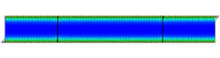
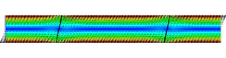
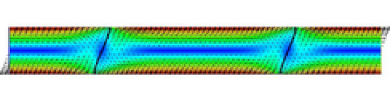
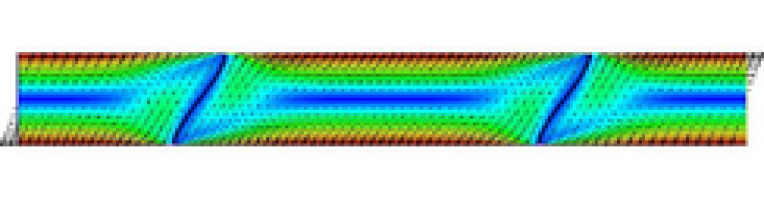
Figure 9: Velocity field at t=1, 10, 20, 100 in the symmetric case. The color represents the velocity magnitude.

More quantitatively, Figure 10 shows the velocity on the top wall at $t=5$ (the contact points are still moving) and at $t=160$ (the contact points are fixed). Figure 11 shows the evolution in time of the velocity of a point on the contact line (which tends to zero) and of the velocity of a point on the wall far from the contact line (which tends to about $0.21$, whereas a total adherence would correspond to $0.25$). The stationary interfaces in the symmetric and asymmetric cases are represented on Figure 12. These results are in very good agreement with those presented in [17], which were obtained either by a continuum phase-field formulation, or by molecular dynamics simulations.

Figure 10: Velocity on the top wall versus $x$ for the symmetric case. At $t=5$, we are still in the transient phase, the velocity of the points on the contact line is non-zero. At $t=160$, the points on the contact line are almost fixed (which means they indeed move with respect to the wall), whereas the points on the boundary far from the contact line move with a velocity of magnitude about $0.21$ ($0.25$ would have meant a complete adherence on the wall).

Figure 11: Velocity of the point C1 on the contact line and of the point A on the boundary (see Figure 8) versus time for the symmetric case. The velocity of the point on the contact line tends to zero (pure slip) whereas the velocity of the point A tends to about $0.21$.

Figure 12: Stationnary interface profiles in the symmetric and asymmetric cases.

To illustrate the result established in Proposition 3, we performed the above experiment with three values of surface tension $\gamma=5.5,11,55$ and we plot in Figure 13, the quantity:

$$\begin{array}[t]{l}\displaystyle{\frac{K^{n+1}-K^{n}}{\delta t}}+\displaystyle{\frac{W^{n+2}-W^{n+1}}{\delta t}}+P_{v}^{n+1}+\gamma\displaystyle{\frac{|\Sigma^{n+2}|-|\Sigma^{n+1}|}{\delta t}}+\beta({\boldsymbol{u}}^{n+1}-{\boldsymbol{u}}_{b},{\boldsymbol{u}}^{n+1})_{\partial\Omega}\\[9.0pt] \leavevmode\nobreak\ \leavevmode\nobreak\ \leavevmode\nobreak\ \leavevmode\nobreak\ \leavevmode\nobreak\ \leavevmode\nobreak\ \leavevmode\nobreak\ \leavevmode\nobreak\ +\displaystyle{\int_{\Omega^{n}}}\displaystyle{\frac{\rho}{2\delta t}}|{\boldsymbol{u}}^{n+1}-{\boldsymbol{u}}^{n}|^{2}-\gamma\int_{\partial\Sigma^{n+1}}\cos(\theta_{s}){\boldsymbol{t}}_{\partial\Omega}\cdot{\boldsymbol{u}}^{n+1}\,dl_{\partial\Sigma}.\end{array}$$ (64)

According to Proposition 3, this quantity is equal to $\epsilon_{\gamma,exp}^{n+1}$ (defined in (52)). The results presented in Figure 13 confirm that the surface tension indeed generates spurious power (the balance is positive), which increases with the surface tension coefficient $\gamma$.

Figure 13: Effect of surface tension on the energy balance (64) when the interface displacement is treated explicitly. Observe that this quantity is indeed positive and increases with the surface tension coefficient $\gamma$ (at least in the dynamic part of the simulation when the interface is still significantly moving). This confirms the results of Proposition 3.

7 Conclusion

We have proposed a formulation for the Generalized Navier Boundary Condition which allows to compute the moving contact line at the interface between two fluids. This formulation is in particular well-suited to an energy stability analysis. We have shown that an explicit treatment of the free interface displacement introduces a spurious power in presence of gravity and surface tension. The study of the surface tension terms required an extension of the Geometric Conservation Law concept to surface integrals. Several stability results have been established and illustrated with numerical experiments. Understanding the spurious power induced by numerical schemes may help to devise more stable algorithms. In particular, we have proposed a simple scheme which offers a good compromise between efficiency, stability and artificial diffusion.

Extension to second order schemes and generalization to more general cases of the “Surface Geometric Conservation Law” (Lemma 4) could be investigated in future works.

References

- [1] L. Ambrosio and H.M. Soner. Level set approach to mean curvature flow in arbitrary codimension. J. Differential Geom., 43(4):693–737, 1996.
- [2] M.C. Delfour and J.-P. Zolésio. Shapes and Geometries. Advances in design and control. SIAM, 2001.
- [3] M.S. Engelman, R.L. Sani, and P.M. Gresho. The implementation of normal and/or tangential velocity boundary conditions in finite element codes for incompressible fluid flow. Int. J. Num. Meth. Fluids, 2(3):225–238, 1982.
- [4] A. Ern and J.-L. Guermond. Theory and practice of finite elements. Springer Verlag, 2004.
- [5] L. Formaggia and F. Nobile. A stability analysis for the arbitrary Lagrangian Eulerian formulation with finite elements. East-West J. Numer. Math., 7(2):105–131, 1999.
- [6] J.-F. Gerbeau, C. Le Bris, and T. Lelièvre. Simulations of MHD flows with moving interfaces. J. Comput. Phys., 184:163–191, 2003.
- [7] J.-F. Gerbeau, C. Le Bris, and T. Lelièvre. Mathematical methods for the Magnetohydrodynamics of liquid metals. Oxford University Press, 2006.
- [8] V. Girault and P.-A. Raviart. Finite element methods for Navier-Stokes equations. Springer-Verlag, 1986.
- [9] D. Gueyffier, J. Li, A. Nadim, S. Scardovelli, and S. Zaleski. Volume of fluid interface tracking with smoothed surface stress methods for three-dimensional flows. J. Comput Phys., 152:423–456, 1999.
- [10] H. Guillard and C. Farhat. On the significance of the geometric conservation law for flow computations on moving meshes. Comput. Methods Appl. Mech. Engrg., 190(11-12):1467–1482, 2000.
- [11] N. G. Hadjiconstantinou. Combining atomistic and continuum simulations of contact-line motion. Phys. Rev. E, 59:2475–2478, 1999.
- [12] N. G. Hadjiconstantinou. Hybrid atomistic-continuum formulations and the moving contact-line problem. J. Comput. Phys, 154:245–265, 1999.
- [13] C.W. Hirt and B.D. Nichols. Volume of fluids (VOF) method for the dynamics of free boundaries. J. Comput. Phys., 39:201–225, 1981.
- [14] M. Lesoinne and C. Farhat. Geometric conservation laws for flow problems with moving boundaries and deformable meshes and their impact on aeroelastic computations. Computer Methods in Applied Mechanics and Engineering, 134:71–90, 1996.
- [15] B. Nkonga and H. Guillard. Godunov type method on nonstructured meshes for three-dimensional moving boundary problems. Comput. Methods Appl. Mech. Engrg., 113(1-2):183–204, 1994.
- [16] T.Z. Qian, X.P. Wang, and P. Sheng. Molecular scale contact line hydrodynamics of immiscible flows. Phys. Rev. E, 68:016306, 2003.
- [17] T.Z. Qian, X.P. Wang, and P. Sheng. Molecular hydrodynamics of the moving contact line in two-phase immiscible flows immiscible flows. Commun. Comput. Phys., 1(1):1–52, 2006.
- [18] W. Ren and W. E. Boundary conditions for the moving contact line problem. Phys. fluids, 19(2):022101, 2007.
- [19] J.A. Sethian and P. Smereka. Level set methods for fluid interfaces. Annual Review of Fluid Mechanics, 35:341–372, 2003.
- [20] Y.D. Shikhmurzaev. Moving contact line in liquid/liquid/solid systems. J. Fluid. Mech., 334:211–249, 1997.
- [21] A. Soulaïmani and Y. Saad. An arbitrary Lagrangian-Eulerian finite element method for solving three-dimensional free surface flows. Comput. Meth Appl. Mech Engrg., 162:79–106, 1998.
- [22] M. Sussman, P. Smereka, and S. Osher. A level set approach for computing solutions to incompressible two-phase flow. J. Comput. Phys., 114:146–159, 1994.
- [23] R. Temam. Navier-Stokes Equations, Theory and Numerical Analysis. North-Holland, 1979.
- [24] P. A. Thompson and M. O. Robbins. Microscopic studies of static and dynamic contact angles. J. Adhesion Sci. Technol., 7(6):535–554, 1993.
- [25] C.E. Weatherburn. Differential geometry of three dimensions, volume 1. Cambridge University Press, 1947.