Bouncing ball orbits and symmetry breaking effects in a three-dimensional chaotic billiard

Abstract

We study the classical and quantum mechanics of a three-dimensional stadium billiard. It consists of two quarter cylinders that are rotated with respect to each other by 90 degrees, and it is classically chaotic. The billiard exhibits only a few families of nongeneric periodic orbits. We introduce an analytic method for their treatment. The length spectrum can be understood in terms of the nongeneric and unstable periodic orbits. For unequal radii of the quarter cylinders the level statistics agree well with predictions from random matrix theory. For equal radii the billiard exhibits an additional symmetry. We investigated the effects of symmetry breaking on spectral properties. Moreover, for equal radii, we observe a small deviation of the level statistics from random matrix theory. This led to the discovery of stable and marginally stable orbits, which are absent for unequal radii.

I Introduction

Wave chaotic phenomena are visible in a large variety of physical systems ranging from lattice QCD V94 ; VW00 to nuclei Brody81 , atoms Friedrich , mesoscopic systems Mirlin , optical microcavities Noeckel , microwave resonators Stock ; Sridhar ; R1 , and to vibrations of macroscopic objects Weav ; Elle . The correspondence between the classical dynamics and wave phenomena in the semiclassical regime is of particular interest in such systems; for a comprehensive review, we refer the reader to Ref. QC ; GMW . It is best understood in Hamiltonian systems with two degrees of freedom, whereas there is a lack of studies of chaotic three-dimensional systems. Experimental investigations of wave chaotic phenomena in three dimensions can be performed with microwave resonatorsDeus ; Wirzba ; SinaiExp and acoustic blocks Weav ; Elle . The resonance spectra investigated in such experiments are described by non-scalar wave equations and are considerably more complicated than the quantum mechanical wave equations of a non-integrable Hamiltonian system with three degrees of freedom.

Let us briefly review the (relatively short) list of studies of quantum chaos in three-dimensional billiards. Prosen investigated quantum chaotic phenomena in a three-dimensional deformed sphere Prosen . Primack and Smilansky PS unraveled the classical and quantum mechanics of the three-dimensional Sinai billiard Sinai , and verified the applicability of Gutzwiller’s trace formula Gutz ; Gutzwiller ; a corresponding experimental study of a microwave resonator was presented in Ref. SinaiExp . The experimental study Richt of the three-dimensional Bunimovich stadium led to a verification of the trace formula proposed by Balian and Duplantier BaDu for electromagnetic systems. A self-bound three-body system with high-dimensional scars was studied theoretically in Ref. PP . Problems involving mode coupling in three-dimensional systems were investigated in vibrating crystals Elle and also in a microwave resonator Richt .

The theoretical description of quantum chaos in three-dimensional systems is in general very difficult. A full understanding of the classical dynamics is compounded by the difficulty to visualize motion in phase space. Moreover, the analysis of level statistics of the corresponding quantum system requires the accurate computation of long level sequences and can be a very time-consuming task for eigenstates with short wave lengths. Furthermore, there are a number of open questions. These concern, for instance, the applicability and accuracy of semiclassical periodic orbit sums for the quantization of such systems. This problem was addressed by Primack and Smilansky in their study of the three-dimensional Sinai billiard PS , which is completely chaotic. Yet, an infinite number of families of marginally stable (bouncing ball) orbits considerably complicates the semiclassical computation of the level density in terms of Gutzwiller’s trace formula. For the evaluation of the resonance density in three-dimensional microwave resonators, Gutzwiller’s trace formula does not apply, and one has instead to use the trace formula by Balian and Duplantier. The applicability of this periodic orbit sum was recently investigated and confirmed for a three-dimensional stadium billiard with chaotic dynamics Richt . It is the purpose of the present work to study the quantum mechanical aspects of the three-dimensional stadium billiard further. We will focus in particular on quantum manifestations of classical chaos, the applicability of Gutzwiller’s periodic orbit sum, and on effects related to symmetry breaking.

The billiard depicted in Fig. 1 is a generalization of the two-dimensional Bunimovich stadium Bunimovich to three dimensions Stadium3D . It consists of two quarter cylinders that are rotated about 90 degrees with respect to each other. For the case that these quarter cylinders are separated by a finite distance $a$, Bunimovich and Del Magno Bun06 showed that this billiard is completely hyperbolic, i.e. there is no finite measure of trajectories that is not exponentially sensitive to changes of their initial conditions. Earlier numerical studies suggest that the billiard of Fig. 1 is also classically chaotic Stadium3D . In what follows, we restrict ourselves to this case.

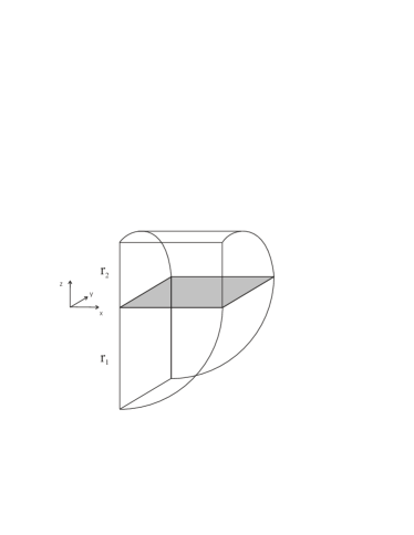
Figure 1: (Color online) Three-dimensional stadium billiard. The plane $z=0$ is shaded.

There are several reasons why the three-dimensional stadium billiard is a promising candidate for the study of quantum chaos. First, the classical dynamics is strongly chaotic and no stable islands are known for $r_{1}\neq r_{2}$. In this work, we focus particularly on the case $r_{1}=\sqrt{2}r_{2}$ since this geometry was studied in microwave experiments Richt and in Ref. Stadium3D . The ratio was chosen irrational in order to avoid nongeneric quantum effects due to classical orbits of measure zero (see below). Second, nongeneric contributions to the level density arise due to two families of bouncing-ball orbits. However, unlike in the case of the three-dimensional Sinai billiard PS , their contribution can be computed and subtracted. Third, for $r_{1}=r_{2}$ the billiard exhibits a high symmetry (under reflection at the $z=0$ plane with a subsequent rotation around the $z$-axis about $90$ degrees), and this offers the opportunity to study symmetry-breaking effects. Below, we will see that the level statistics in this highly symmetric case exhibit a deviation from the theoretical prediction for chaotic systems. This led to the discovery of a stable and a few marginally stable orbits which were previously unknown.

This article is organized as follows. In Sect. II, we focus on classical periodic orbits and nongeneric modes. In Sect. III, we present our analysis of the quantum mechanical spectra and discuss level statistics and symmetry breaking. We conclude with a summary of the main results. Some technical aspects concerning the finite element approximation with web-splines are deferred to the Appendix.

II Nongeneric modes and periodic orbits

In this section we investigate nongeneric modes and classical periodic orbits. The former are an interesting, system-specific property and must be subtracted from the staircase function before generic properties can be analyzed; the latter are useful in a semiclassical interpretation of quantum spectra.

II.1 Nongeneric modes

We study the desymmetrized stadium billiard depicted in Fig. 1. The dynamics is limited to $x\geq 0$ and $y\geq 0$ with specular reflections at the planes $x=0$ and $y=0$. We use $r_{1}\geq r_{2}$ and will express lengths in units of $r_{2}$ and wave momenta in units of $r_{2}^{-1}$. For $r_{1}\neq r_{2}$, the billiard is fully desymmetrized; for $r_{1}=r_{2}$, it is still symmetric under reflection at the plane $z=0$ and a subsequent rotation by $\pi/2$ around the $z$-axis. We label eigenstates by their wave momentum $k$. Employing a recently developed method which is based on finite elements and seeks solutions of the Schrödinger equation with Dirichlet boundary conditions, we computed the lowest 1200 levels up to $kr_{2}\approx 35$. More details on this method are given in the appendix.

The staircase function

$$N(k)=\sum_{n=1}^{X}\Theta(k-k_{n})$$ (1)

with $\Theta(x)$ denoting the unit step function counts the levels below a given $k$. It is the sum of a smooth part $N_{\rm smooth}(k)$ and a fluctuating part $N_{\rm fluc}(k)$, i.e., $N(k)=N_{\rm smooth}(k)+N_{\rm fluc}(k)$. The smooth part is given by the Weyl formula which is a polynomial of degree three in $k$, and is subtracted from $N(k)$. Figure 2 shows the remaining fluctuating part. One identifies large-scale oscillations that grow in amplitude with increasing wave momentum. These fluctuations are due to the nongeneric modes of the billiard associated with the bouncing-ball orbits perpendicular to the flat boundaries of the billiard and the orbits within the $z=0$ plane.

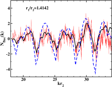
Figure 2: (Color online) Fluctuating part $N_{\rm fluc}$ of the staircase function for the geometry with $r_{1}/r_{2}=\sqrt{2}$ (thin line). Contributions from bouncing-ball orbits (dashed line) and from all nongeneric modes (thick line).

The fluctuating part of the level density is obtained by differentiation, i.e. $\rho_{\rm fluc}(k)={d\over dk}N_{\rm fluc}(k)$. The absolute value squared of the Fourier transform of this quantity yields the length spectrum. It is shown in the upper part of Fig. 3 for $r_{1}=\sqrt{2}r_{2}$. The peaks in the length spectrum appear at the lengths of classical periodic orbits Gutzwiller . The most prominent peaks are at lengths that are multiples of the bouncing-ball orbits with lengths $2r_{1}$ and $2r_{2}$, respectively. There are other peaks that can be identified with the lengths of orbits inside the rectangular $z=0$ plane. Both types of orbits are nongeneric due to their particular stability properties. As we are interested in generic properties, we have to extract these contributions.

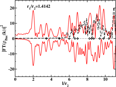
Figure 3: (Color online) Upper part: Length spectrum of the three-dimensional stadium billiard for $r_{1}/r_{2}=\sqrt{2}$ (full line). Contributions from unstable periodic orbits (dashed line). Lower part: Sum of contributions from nongeneric modes and unstable periodic orbits (full line). Peaks at multiples of $2r_{1}$ and $2r_{2}$ correspond to the bouncing-ball orbits in the two quarter cylinders. Diamonds: Lengths of nongeneric orbits in the $z=0$ plane.

First, let us consider the bouncing-ball orbits. There are two families of bouncing-ball orbits which bounce back and forth between the two parallel planes of distance $r_{1}$ and $r_{2}$ in the two quarter cylinders, respectively. These orbits are marginally stable as they have zero Lyapunov exponents. According to semiclassical periodic orbit theory, they are associated with long-range oscillations of the quantum mechanical density of states.

We follow Ref. Wirzba for the computation of the contribution of bouncing-ball orbits to the staircase function, and focus on the bouncing-ball modes in the upper quarter cylinder first. The number of bouncing-ball (bb) modes up to momentum $k$ is given by

$$N_{\rm bb}(k) = {\rm Tr}_{{\rm bb}}\Theta\left({\hbar^{2}k^{2}\over 2m}-\hat{H}\right)$$ (2)

$$= \int{dzdk_{z}\over 2\pi}\int{dydk_{y}\over 2\pi}\sum_{\mu=1}^{\infty}$$

$$\Theta\left(k^{2}-k_{z}^{2}-k_{y}^{2}-k_{x,\mu}^{2}\right)$$

$$+ \left((x,y)\to(y,x)\right)\ .$$

Here,

$$k_{x,\mu}\equiv{\mu\pi\over l_{x}}\ ,$$ (3)

and $l_{x}=r_{1}$, $l_{y}=r_{2}$. This ansatz for the number of bouncing-ball modes is intuitively clear. The trace is performed in the semiclassical approximation as a phase space integral in the directions perpendicular to the bouncing-ball orbits, while these modes are quantized along the orbit. The integrations can be performed, and one obtains Wirzba

$$N_{\rm bb}(k) = {r_{1}^{2}\over 16}\sum_{\mu\geq 1}\left(k^{2}-k_{2,\mu}^{2}\right)\Theta\left(k^{2}-k_{2,\mu}^{2}\right)$$ (4)

$$+ {r_{2}^{2}\over 16}\sum_{\mu\geq 1}\left(k^{2}-k_{1,\mu}^{2}\right)\Theta\left(k^{2}-k_{1,\mu}^{2}\right)\ .$$

To obtain the fluctuating contribution $N_{\rm bb,fluc}$, we subtract a polynomial of third degree in $k$ from the expression (4). We confirmed that the leading coefficients of this polynomial agree with the coefficients of the Weyl formula. An analytical formula is presented in Ref. Wirzba . As evident from Fig. 2, the bouncing-ball orbits (dashed line) describe the gross oscillations of the fluctuating staircase function rather well. To account for finer details, we also have to consider nongeneric modes inside the $z=0$ plane.

The rectangular $z=0$ plane is special, since the classical motion is regular inside this plane but unstable with respect to deviations out of this plane. Note that this does not spoil the hyperbolicity of the billiard since the set of orbits restricted to the $z=0$ plane are of measure zero in classical phase space. However, remnants of families of classical orbits inside this plane can also be associated with long-range fluctuations in the quantum mechanical level density for the following two reasons. First, the periodic orbits inside this plane come in two-dimensional families opposed to the isolated periodic orbits in hyperbolic systems. Second, these orbits are less unstable than most truly three-dimensional periodic orbits and thus enter any periodic-orbit sum with a greater weight. It is thus necessary to include the nongeneric modes associated with the $z=0$ plane.

Extending the results from Ref. Wirzba , the number of modes associated with nongeneric orbits is given by the quantum mechanical trace over nongeneric (ng) modes

$$N_{\rm ng}(k) = {\rm Tr}_{{\rm ng}}\Theta\left({\hbar^{2}k^{2}\over 2m}-\hat{H}\right)$$

$$= \int{dzdk_{z}\over 2\pi}\sum_{\mu,\nu=1}^{\infty}\Theta\left(k^{2}-k_{z}^{2}-k_{x,\mu}^{2}-k_{y,\nu}^{2}\right)\ .$$

This ansatz is again transparent: the trace is approximated by a phase-space integral in the $z$-direction, while the rectangular sections (with $z$-dependent area) perpendicular to the $z$-axis are explicitly quantized. We thus quantize the motion inside this plane adiabatically, quite similar to the approach that Bai et al. Taylor applied to the Bunimovich stadium. Note that Eq. (II.1) accounts both for the bouncing-ball orbits and for the modes associated with the $z=0$ plane.

In Eq. (II.1), the wave momenta $k_{x,\mu}$ and $k_{y,\nu}$ are defined as in Eq. (3) but with the $z$-dependent radii $l_{x}$ and $l_{y}$. We have

$$l_{x}(z) = \left\{\begin{array}[]{ll}r_{1}&\mbox{for $z<0$},\\ \sqrt{r_{1}^{2}-z^{2}}&\mbox{for $z\geq 0$}.\end{array}\right.$$ (8)

$$l_{y}(z) = \left\{\begin{array}[]{ll}r_{2}&\mbox{for $z\geq 0$},\\ \sqrt{r_{2}^{2}-z^{2}}&\mbox{for $z<0$}.\end{array}\right.$$ (11)

The integrations in Eq. (II.1) can be performed analytically, and one obtains

$$N_{\rm ng}(k)={1\over\pi}{\sum_{\mu,\nu\geq 1}}^{\prime}\left(A(\kappa_{\mu\nu},r_{1},r_{2})+A(\kappa_{\mu\nu},r_{2},r_{1})\right)\ .$$ (12)

Here

$$A(\kappa_{\mu\nu},r_{1},r_{2}) \equiv r_{1}\sqrt{\kappa^{2}_{\mu\nu}-k_{2,\nu}^{2}}$$ (13)

$$\left(E(\kappa_{\mu\nu})-(1-\kappa^{2}_{\mu\nu})K(\kappa_{\mu\nu})\right)\$$

with

$$\kappa_{\mu\nu}=\kappa_{\mu\nu}(k,r_{1},r_{2})\equiv\left({k^{2}-k_{1,\mu}^{2}-k_{2,\nu}^{2}\over k^{2}-k_{2,\nu}^{2}}\right)^{1/2}\$$ (14)

contains the dependence on the wave momentum and the radii of the billiard. The wave momenta $k_{1,\mu}$ and $k_{2,\nu}$ are defined in Eq. (3). In Eq. (13), $K(\kappa)$ and $E(\kappa)$ are the complete elliptical integrals of the first and second kind, respectively. The prime in the sum of Eq. (12) indicates that the summation is limited to values of $\mu,\nu$ such that the square roots in Eqs. (13) and (14) are real.

The smooth part of the staircase function is again a polynomial of degree three and is subtracted. The fluctuating part of $N_{\rm ng}(k)$ is shown in Fig. 2 as a thick line. Clearly, the gross and also finer oscillations are accounted for. This enables us to analyze the length spectra depicted in Fig. 3. The upper part shows the length spectra, i.e. the Fourier transform of the fluctuating part of the density of states, the lower part that of the nongeneric modes and the unstable periodic orbits, which has been computed based on Eq. (12) and the Gutzwiller trace formula (see next section). The peaks at multiples of the lengths $2r_{1}$ and $2r_{2}$ are due to the bouncing-ball modes. The peaks marked by a diamond are due to the nongeneric orbits in the $z=0$ plane. The remaining peaks must thus be associated with lengths of isolated periodic orbits, and we turn to their analysis in the following subsection.

II.2 Unstable periodic orbits

Following Gutzwiller’s periodic orbit theory Gutzwiller , the semiclassical approximation of the quantum mechanical density of states is given in terms of the periodic orbits of the underlying classical system. This sum is infinite such that approximations have to be invoked. Here, we are interested in the length spectrum, i.e. the power spectrum of the Fourier transform of the fluctuating part of the level density. The length spectrum up to length $l$ is given in terms of all periodic orbits up to length $l$, and this is a finite (but usually with $l$ exponentially increasing) number of periodic orbits.

The search for periodic orbits is a cumbersome task. Here, we use two different methods and focus on periodic orbits outside the $z=0$ plane. The first method considers the Poincaré surface of section (PSOS) defined by $z=0,p_{z}>0$, and constructs the PSOS map. Periodic orbits are fixed points of this map. They are found by starting a large number of trajectories in the PSOS and by using a Newton-Raphson algorithm to find fixed points in the vicinity of each such trajectory.

The second method is based on a symbolic code and utilizes the fact that the length of a periodic orbit is a local extremum under variation of the points of reflection along the billiard’s boundary. This procedure is similar to the one described in Ref. PS . We consider an open billiard system which is the infinite periodic extension of our billiard, and assign the letters “+” and “-” to reflections on the curved parts of the upper and lower quarter cylinder, respectively. Periodic orbits outside the $z=0$ plane can certainly be described as words composed from these two letters. We have no proof that there is a one-to-one correspondence between this symbolic code and the periodic orbits of our system. Given a word from this alphabet, we construct a random closed orbit as follows. For each “+” (“-”) letter of the word, we choose a random point on the curved surface of the upper (lower) quarter cylinder. We connect this sequence of points by straight lines and compute the length of this closed orbit. Then we vary the positions of the random points in order to find a local minimum of the length.

Both methods yield a considerable number of periodic orbits, and we consider the union of the resulting sets as our set of periodic orbits. Once a periodic orbit is found, we compute its length, monodromy matrix and its Maslov index following Ref. Sieber . Recall that the monodromy matrix is the tangent map and encodes the stability properties of the periodic orbit. For unstable orbits, its eigenvalues come in real pairs $\Lambda_{+},\Lambda_{-}$ with $\Lambda_{+}\Lambda_{-}=1$ or in complex quadruples $\Lambda_{+},\Lambda_{-},\Lambda_{+}^{*},\Lambda_{-}^{*}$ with $\Lambda_{+}\Lambda_{-}=1$. Stable orbits have two pairs of complex eigenvalues with modulus one.

We performed our most extensive search for the billiard with the geometry $r_{1}=\sqrt{2}r_{2}$ and determined more than 2000 periodic orbits. We believe that our list is fairly complete for the shortest orbits. All periodic obits we found were unstable. This extends and confirms the numerical results of Ref. Stadium3D and strongly suggests that the billiard is completely chaotic. The quantum mechanical results presented below support this picture. The contribution of the unstable periodic orbits to the length spectrum is shown in the upper part of Fig. 3 as a dashed line. Clearly, unstable periodic orbits contribute significantly to the length spectrum, particularly for length $l/r_{2}\gtrsim 6$ where the contributions from nongeneric modes become less dominant.

However, for the case $r_{1}=r_{2}$ we found a stable periodic orbit. This was unexpected, since earlier studies Stadium3D yielded a positive Lyapunov exponent for a sample of $10^{4}$ randomly chosen trajectories, and not one of the trajectories was found to be stable. The shortest stable periodic orbit we found has a length $l/r_{2}\approx 10.1706$. Note that the eigenvalues of the monodromy matrix corresponding to this orbit are on the unit circle and very close to the real axis. Thus it is difficult to distinguish this orbit from a marginally stable orbit. We also obtained periodic orbits (in addition to the bouncing-ball orbits) that are marginally stable, i.e. the eigenvalues of the monodromy matrix are real with modulus one. The shortest of these orbits has a length $l/r_{2}\approx 5.4981$. Other marginally stable orbits have periods $l/r_{2}\approx 5.5153,6.2701,6.4738$.

To study the relevance of these orbits, we show the length spectrum of the billiard for $r_{1}=r_{2}$ in Fig. 4. Diamonds denote the lengths of bouncing-ball orbits and of nongeneric periodic orbits associated with the $z=0$ plane; they account for many peaks in the length spectrum. We also computed the lengths, monodromy matrices and Maslov indices of the 400 shortest unstable and marginally stable orbits by proceeding as in the case $r_{1}=\sqrt{2}r_{2}$. However, we have no semiclassical theory for the computation of the density of states for the marginally stable and the stable orbit, and we are not able to disentangle their contribution to the length spectrum from that of the nongeneric modes. For this reason we show in Fig. 4 the length spectrum of the billiard and indicate the lengths of the nongeneric orbits by diamonds, and those of the marginally stable orbits by the full arrows. The dashed arrow marks the length of the stable orbit. It is difficult to clearly identify its impact on the length spectrum, since the peak around length $l/r_{2}\approx 10.19$ can be attributed to the stable orbit and/or to a nongeneric orbit. Recall that a stable orbit leaves a strong imprint in the length spectrum if the stable island around it is sufficiently large (in units of $(2\pi\hbar)^{3}$) to accommodate eigenstates. To obtain an estimate for the phase-space volume of the elliptical island we started bundles of $21^{4}$ trajectories in the PSOS close to the stable periodic orbit. All trajectories departed from the stable orbit after a few intersections with the PSOS. Within the achievable numerical accuracy we may thus conclude, that either the volume of the phase space associated with the stable orbit is very small or that contrary to our numerical results it is only marginally stable. Note that there are several marginally stable orbits associated with the third arrow from the left. These orbits have almost identical lengths, and the visual inspection indicates that they are whispering gallery orbits. In this case, interference effects might explain why there is no clear peak in the length spectrum associated with these orbits. A similar effect has been found in the two-dimensional stadium billiard Sie . In the next section we present evidence that the stable and marginally stable orbits explain peculiarities in the level statistics of the billiard with $r_{1}=r_{2}$.

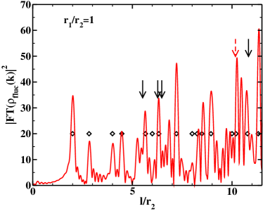
Figure 4: (Color online) Full line: Length spectrum for $r_{1}=r_{2}$. Diamonds: Length of bouncing-ball orbits and of nongeneric orbits in the $z=0$ plane. Full arrows: Length of marginally stable orbits. Dashed arrow: length of stable periodic orbit.

III Spectral properties and symmetry breaking

In this section we investigate statistical properties of the eigenvalues of the three-dimensional stadium billiard for a varying ratio of the radii $r_{1}/r_{2}$ of the two quarter cylinders, where the volume of the billiard is kept fixed. We computed the lowest 1200 levels with a recently developed finite element method Moessner described in the appendix. The lowest 200 levels are discarded since we are interested in the correspondence between classical and quantum mechanics. In order to get rid of system-dependent properties, we need to rescale the eigenvalues to unit mean spacing and to extract the contributions of the nongeneric modes to the fluctuating part of the resonance density. This is done by replacing the computed wave numbers $k$ by $\tilde{k}=N_{\rm smooth}(k)+N_{\rm ng,fluc}(k)$ (see R1 ; Wirzba ). As the underlying classical dynamics is completely chaotic, we expect agreement of the statistical properties of the unfolded eigenvalues with those of random matrices drawn from the Gaussian orthogonal ensemble (GOE) if $r_{1}$ is chosen not equal to $r_{2}$ bgs . In Fig. 5 we show the nearest-neighbor spacing distribution and the $\Sigma^{2}$-statistics for a ratio of radii $r_{1}/r_{2}=\sqrt{2}$, i.e. for the case considered in the experiments with the microwave cavity of the shape of a three-dimensional stadium billiard Richt . Both curves agree well with the corresponding ones for random matrices from the GOE. This shows that first the three-dimensional quantum stadium billiard behaves like a generic quantum system with chaotic classical dynamics, and second that our procedure of extracting the contribution of nongeneric modes is applicable and complete.

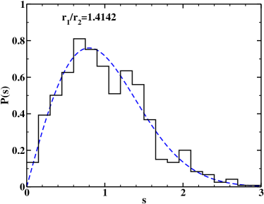
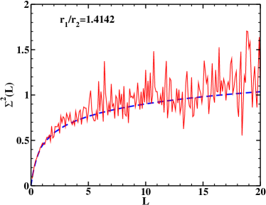
Figure 5: (Color online) Upper panel: Nearest neighbor spacing distribution (histogram) of the billiard for $r_{1}=\sqrt{2}r_{2}$ compared to the GOE prediction (dashed line). Lower panel: $\Sigma^{2}$-statistics (thin line) compared to the GOE prediction (dashed line).

We recall that the experiment Richt with a microwave resonator of the shape of a three-dimensional stadium billiard with $r_{1}/r_{2}=\sqrt{2}$ revealed deviations of the spectral properties from GOE-behavior. This was attributed to a partial decoupling between electromagnetic TE and TM modes in the low-frequency regime. Note, however, that this system differs from the quantum billiard considered in the present work due to the vectorial character of the underlying wave equations. As a consequence, the trace formula by Balian and Duplantier BaDu has to be employed for the semiclassical computation of the length spectrum. It differs from Gutzwiller’s trace formula in the occurrence of a factor associated with the polarization, and as a consequence, only periodic orbits with an even number of reflections enter. The evaluation of this factor showed that the electric and magnetic modes are decoupled on a considerable fraction of the short periodic orbits. This finding supports the interpretation of the observed deviations from GOE-behavior in terms of a partial decoupling between the TE and the TM modes. In Richt the experimental length spectrum was well reproduced by the theoretical calculations based on the trace formula derived by Balian and Duplantier. As there the polarization of the electric field is taken into account for each unstable periodic orbit individually, this good agreement is not in contradiction to the discrepancy obtained for the spectral properties.

III.1 Symmetry breaking

For $r_{1}=r_{2}$, the billiard is symmetric with respect to reflections at the $z=0$ plane and a subsequent $\pi/2$-rotation about the $z$-axis. Accordingly, in this case the wave functions of the billiard are symmetric or antisymmetric under the symmetry operation and belong to different irreducible representations (IR). Assuming that the billiard is chaotic, the spectral properties of levels within each IR are expected to coincide with those of random matrices from the GOE. However, the spectral statistics for the whole set of eigenvalues should coincide with RMT for a superposition of two independent GOEs.

Let $H_{1}$ and $H_{2}$ be two random matrices drawn from the GOE and consider an ensemble of random matrices of the form GMW ; Rosen ; Leitner

$$H=\pmatrix{H_{1}&0\cr 0&H_{2}\cr}\,.$$ (15)

For a generic chaotic system with two symmetry classes, the spectral properties of the eigenvalues associated with each symmetry class are given by those of the random matrices $H_{1}$ and $H_{2}$, respectively, whereas the complete set of eigenvalues is described by those of $H$ itself. Since, in our case, the number of eigenvalues associated with the two symmetry classes are (approximately) equal, the matrices $H_{1}$ and $H_{2}$ are chosen of equal dimension for the theoretical description of the spectral properties of the quantum billiard. In Fig. 6 we compare the $\Sigma^{2}$-statistics for the eigenvalues of the quantum billiard (thin line) with that of an ensemble of random matrices of the form Eq. (15) (dashed line), which is known analytically Leitner . We observe significant deviations, which cannot be explained by an additional family of nongeneric modes. Indeed, Fig. 7 shows the fluctuating part of the staircase function $N_{\rm fluc}(f)$ for the case $r_{1}=r_{2}$ (thin line) and the contributions of the nongeneric modes resulting from Eq. (12) (thick line). As for the case $r_{1}/r_{2}=\sqrt{2}$, the smooth oscillations of $N_{\rm fluc}(f)$ are well described by our expression. From this we may conclude that the adiabatic method described in Section II yields a good approximation for the contribution of the nongeneric modes to the staircase function also for $r_{1}=r_{2}$. We also verified, that the deviations are not due to insufficient numerical accuracy in the computation of the eigenvalues. How can this puzzle be understood?

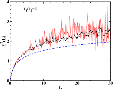
Figure 6: (Color online) $\Sigma^{2}$-statistics for the billiard with $r_{1}=r_{2}$ (thin line) compared to the GOE prediction (dashed line) and to a random matrix model which also includes a Poissonian sequence of random levels (dots).

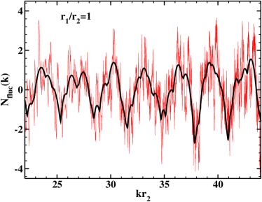
Figure 7: (Color online) The fluctuating part $N_{fluc}$ of the staircase function for the billiard with $r_{1}=r_{2}$ (thin line) compared to the contributions from the nongeneric modes (thick line).

Recall that the billiard has a stable orbit for $r_{1}=r_{2}$ and several marginally stable orbits besides the bouncing ball orbits. This suggests that their presence causes the deviation depicted in Fig. 6. In order to test this hypothesis, we considered the following random matrix ensemble. Each random matrix consists of two block matrices $H_{1}$ and $H_{2}$ of equal dimension that are drawn from the GOE. These model the two symmetry classes of eigenstates associated with the chaotic part of the billiard (see Eq. (15)). An additional diagonal random matrix of much smaller dimension models eigenstates associated with the few stable orbits. This diagonal matrix thus exhibits Poisson statistics. The dimension of the latter matrix was chosen equal to 25, that of $H_{1}$ and $H_{2}$ equal to 250. The $\Sigma^{2}$-statistics of this random matrix model is plotted as a dotted line in Fig 6. It agrees very well with that of the billiard. This suggests that the stable and marginally stable orbits are responsible for the observed deviations from the prediction of standard RMT. Most interestingly, the stable orbits disappear immediately when the ratio $r_{1}/r_{2}$ differs slightly from one.

For geometries $r_{1}\neq r_{2}$, the symmetry of the billiard is broken. The underlying quantum system “sees” this symmetry breaking once the perturbation due to the symmetry breaking is of the order of the mean level spacing, or, alternatively, once the geometric distortions due to the symmetry breaking are of the scale of one wave length. For a completely broken symmetry, RMT predicts agreement of the spectral properties of the billiard with those of one GOE. Quantum mechanically, however, we found that for $r_{1}\approx r_{2}$, the spectral properties coincide with those of random matrices applicable to chaotic systems with a partially broken symmetry  GMW ; Rosen ; Leitner ; Alt ; SymBrech ,

$$H=\pmatrix{H_{1}&0\cr 0&H_{2}\cr}\,+\sqrt{\lambda}D\pmatrix{0&V\cr V^{T}&0\cr}\,\ .$$ (16)

In this random matrix model, the first (second) matrix preserves (breaks) the symmetry. The size of the symmetry breaking is set by the dimensionless parameter $\lambda$ measured on the scale of the mean spacing $D$. Here as in Eq. (15), $H_{1}$ and $H_{2}$ are random matrices drawn from the GOE. The symmetry breaking is modeled by the off–diagonal blocks $V$ and $V^{T}$, where the random matrix $V$ is real with no symmetries. For this random matrix model, the $\Sigma^{2}$-statistics is known analytically for arbitrary values of $\lambda$.

Figure 8 shows the $\Sigma^{2}$-statistics (thin line) for an increasing ratio $r_{1}/r_{2}$ of the radii of the billiard. For comparison, we also show the $\Sigma^{2}$-statistics for one GOE (dashed line), for two GOEs (dotted line), and for the random matrix model (16) (thick line). The values of $\lambda$ given in the figure are obtained by a fit of the model (16) to the data. For $r_{1}/r_{2}=1.0025$ there is perfect agreement with the random matrix model Eq. (15) that describes chaotic systems with a conserved symmetry. On the one hand, the ratio $r_{1}/r_{2}=1.0025$ deviates (sufficiently strong) from one and the stable island has disappeared. On the other hand, this ratio is still so close to one that the quantum mechanics is unable to resolve the symmetry breaking. For increasing values of the ratio $r_{1}/r_{2}$, the symmetry breaking is revealed in the spectral statistics, and the parameter $\lambda$ in Eq. (16) increases from zero. Eventually, for $r_{1}/r_{2}\approx 1.1\ldots 1.2$, the $\Sigma^{2}$-statistics approaches that of one GOE. This result is in agreement with a semiclassical estimate. The symmetry breaking is resolved for wave lengths $2\pi/k\lesssim|r_{1}-r_{2}|$. We have maximal wave momenta $kr_{2}\approx 35$ and can thus resolve symmetry breaking of the order $r_{1}/r_{2}\gtrsim 1+2\pi/(kr_{2})\approx 1.18$. Note that we can also base our semiclassical estimate on the smooth part $N_{\rm smooth}(k)$ of the staircase function. This function is quadratic in the symmetry-breaking parameter $(r_{1}-r_{2})$. At maximal wave momenta $kr_{2}\approx 35$ nonzero values of this parameter lead to significant changes of $N_{\rm fluc}(k)$ for $r_{1}/r_{2}\gtrsim 1.18$. In conclusion, the classically abrupt change of the symmetry properties of the system is accompanied by a gradual change of the spectral properties of the corresponding quantum system from those of chaotic systems consisting of a superposition of two symmetry classes to those of chaotic systems with no further symmetries.

We add here some more notes concerning the experiment with a microwave resonator Richt . There, the spectral properties were also described with the model given in Eq. (16), where one of the block matrices $H_{1},H_{2}$ depicts the properties of the TE, the other those of the TM modes and deviations from GOE-behavior were interpreted as due to a partial decoupling of them. In the experiment the ratio $r_{1}/r_{2}\simeq\sqrt{2}$ with $r_{1}=200.0$ mm and $r_{2}=141.4$ mm was kept fixed, while the value of the resonance frequency $f$, that is of $k=\frac{2\pi f}{c}$ with $c$ the velocity of light, was varied up to $f=20$ GHz.

Is for this choice of the radii and of the frequency range the symmetry breaking discussed above observable? The breaking of the symmetry existent for $r_{1}=r_{2}$ is resolvable for wavelengths smaller than $|r_{1}-r_{2}|$, that is for $2\pi/k=c/f\lesssim|r_{1}-r_{2}|=58.6$ mm. Accordingly, for excitation frequencies $f\gtrsim 5.12$ GHz good agreement of the spectral properties with those of random matrices from the GOE are expected. In the experiment, however, deviations from one GOE were observed up to approximately 17 GHz. Hence, they cannot be explained with the particular mechanism of symmetry breaking discussed above. In order to resolve the discrepancy between theory and experiment numerical computations of the full vectorial Helmholtz equation are desired.

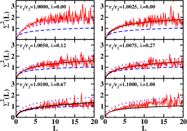
Figure 8: (Color online) $\Sigma^{2}$-statistics for various ratios $r_{1}/r_{2}$ of the billiard (thin line) compared to that of two GOEs (dotted line), one GOE (dashed line), and for the random matrix model in Eq. (15) (thick line).

III.2 High-lying states

Strictly speaking, the semiclassical approximation and the Bohigas-Giannoni-Schmit QC ; BGS ; heusler conjecture, which states, that the spectral fluctuation properties in quantum systems with a chaotic classical dynamics coincide with those of random matrices drawn from the Gaussian random-matrix ensembles, apply in the regime when the wave length is the smallest length scale of the system, i.e. $kr_{2}\gg 1$ must hold. Nevertheless, we saw in the previous section that the semiclassical analysis of the length spectrum is also useful for the low-lying states. In this subsection, we compute high-lying quantum states of the billiard and perform level statistics. For the computation of high-lying levels, we employ Prosen’s generalization Prosen of the two-dimensional method by Vergini and Saraceno Vergini to three-dimensional billiards. This method is particularly suited for high-lying eigenstates and determines a stretch of eigenstates around some arbitrary wave momentum $k_{0}$ with $k_{0}r_{1}\gg 1$. This method yields 1669 levels in the regime $79\lesssim kr_{2}\lesssim 86$.

Figure 9 compares the spectral properties of the eigenvalues in the lowest part of the spectrum (thin line) with those of the high-lying eigenvalues (dashed line) and the GOE (dashed-dotted line). While the $\Sigma^{2}$-statistics of the low-lying set of eigenvalues agrees well with that of random matrices from the GOE, we observe significant deviations for that of the high-lying ones. This points to inadequacies of our procedure to extract the contribution of the nongeneric modes to the fluctuating part of the resonance density. Recall that our semiclassical formula (12) takes account of the leading nongeneric modes. These are contributions that scale as $k^{3}$ with increasing wave momentum. Next-to-leading order contributions scale as $k^{2}$. These are only partly included. In our ansatz (II.1) we integrate over rectangles with a $z$-dependent area. There are many billiards of different shape (but identical volume) that have rectangular cross sections. However, evidently, our procedure is well suited for small or moderate values of $kr_{2}$, but it seems to be insufficient in the semiclassical regime.

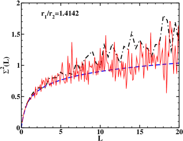
Figure 9: (Color online) $\Sigma^{2}$-statistics of the high-lying stretch of levels around $kr_{2}\approx 80$ (dashed-dotted line) compared to that of the low-lying levels (thin line) and the GOE prediction (dashed line).

IV Summary

We studied the classical and quantum mechanics of the three-dimensional stadium billiard. This billiard consists of two quarter cylinders that are rotated by 90 degrees with respect to each other and is classically chaotic for unequal radii of the quarter cylinders. We studied the nongeneric modes of the billiard that are due to bouncing-ball orbits and orbits within a rectangular cross section of the billiard, and gave analytical expressions for their contribution to the staircase function. The quantum mechanical length spectrum can be understood in terms of the nongeneric modes and unstable periodic orbits. For unequal radii of the two quarter cylinders, the level statistics agrees with predictions from random matrix theory. For equal radii, we found deviations from standard random matrix theory and these can be attributed to a stable and a few marginally stable orbits. We modeled a random matrix ensemble on this basis and found very good agreement with our data. We studied the level statistics as a function of the ratio of the two radii. For slightly unequal radii, there is a sudden transition from a system with mixed phase space to a system with a chaotic phase space. For larger differences of the radii, we follow the symmetry-breaking transition towards the spectral statistics of one GOE.

APPENDIX. FINITE ELEMENT METHOD

In order to calculate a complete sequence of eigenvalues for the three-dimensional stadium billiard, we use a finite element method (see for example Hackbusch , ch. 11). This discretization of the eigenvalue problem

$$\begin{array}[]{rcll}-\Delta\psi_{i}&=&k_{i}^{2}\psi_{i}&\mbox{ in }\Omega,\\ \psi_{i}&=&0&\mbox{ on }\partial\Omega,\end{array}$$ (17)

leads to a generalized eigenvalue problem

$$A^{h}\psi_{i}^{h}=\lambda_{i}^{h}M^{h}\psi_{i}^{h},$$ (18)

where $A^{h},M^{h}\in\mathbb{R}^{n\times n}$ are finite dimensional matrices. The eigenvalues $\lambda^{h}_{i}$ and eigenfunctions $\psi^{h}_{i}$ of the discrete problem approximate the eigenvalues/functions of the continuous problem (17). Here the parameter $h\in\mathbb{R}^{+}$ represents the fineness of the test functions used in the discretization process. With the usual assumptions (see Hackbusch ), we get the error-estimate

$$\lambda^{h}_{i}-\lambda_{i}\leq C\lambda_{i}^{l+1}h^{2l},$$ (19)

where $l$ is the polynomial degree of the used test functions. This estimate shows that it is possible to compute an arbitrary number of eigenvalues with a given accuracy by using a sufficiently fine discretization. Using standard piecewise linear functions, we obtain convergence of order $h^{2}$ so that small values of $h$ are required for high accuracy. Accordingly, the dimension of matrices $A^{h}$ and $M^{h}$ becomes very large, and solving the generalized eigenvalue problem (18) is extremely costly.

Using test functions of higher degree yields a significantly improved performance of the method. We suggest to use a special modification of tensor product B-splines with arbitrary coordinate degree. While, independent of $l$, B-splines may do with only one coefficient per element, standard approaches of higher order require a much larger number, which is increasing with the degree. Since computation time to solve (18) is growing rapidly with the number of degrees of freedom, this aspect is crucial for achieving high accuracy.

So far, despite these advantages, B-splines have rarely been used in finite element applications, the main reasons being Dirichlet boundary conditions and stability. A solution to these problems was proposed by Höllig, Reif and Wipper HRWpaper . Stability is achieved by linking potentially unstable B-splines near the boundary of the domain in an appropriate way to B-splines in the interior of the domain. Following old, but little known ideas of Kantorovitch and Krylow, homogeneous Dirichlet boundary conditions are ensured by multiplying all test functions by a weight function $w$ which vanishes on the boundary and is positive inside the domain $\Omega$. It can be shown that the resulting weighted extended B-splines (web-splines) form a stable basis and possess the same approximation order as the underlying tensor product splines space HRWpaper ; HRWerror ; Hbook .

In this work we apply the WEB-spline method to approximate eigenvalues of the Laplacian on the three-dimensional stadium billiard $\Omega\subseteq\mathbb{R}^{3}$. The implementation includes a specifically designed high accuracy integration algorithm. It is based on precomputed projections of the boundary grid cells and iterated one-dimensional Gauss quadrature.

We use tensor product B-splines of degree $l=4$ on a grid with $25\times 25\times 40$ cells. This leads to a generalized eigenvalue-problem (18) of dimension 9250. To determine the eigenvalues, we use the Cholesky-decomposition $M^{h}=LL^{t}$ to compute the matrix

$$B^{h}:=L^{-1}A^{h}(L^{t})^{-1}.$$ (20)

The eigenvalues of $B^{h}$ are just the generalized eigenvalues of $(A^{h},M^{h})$ so that standard software can be used to compute the $\lambda_{i}^{h}$. Compared with iterative methods, the advantage of this procedure is that one can be sure that no eigenvalues in the domain of interest are lost. On the other hand, the maximal dimension that can be handled that way is limited by the fact that $B^{h}$ is a dense matrix.

Of course, only a certain fraction of the eigenvalues $\lambda_{i}^{h}$ of $B^{h}$ provides a reasonable approximation of some $\lambda_{i}$. The estimate (19) suggests that smaller eigenvalues are approximated better than larger ones, but it does not provide actual bounds since the constant $C$ is not known explicitly. Computations on other domains, where the exact eigenvalues $\lambda_{i}$ are explicitly known, indicate that at least the first $16\%$ of the eigenvalues $\lambda_{i}^{h}$, when ordered my modulus, have a relative error less than $0.1\%$ For the statistical evaluation in this paper, $1200$ out of $9250$ eigenvalues, i.e., $13\%$ are used.

References

- (1) J. J. M. Verbaarschot, Phys. Rev. Lett. 72, 2531 (1994).
- (2) J. J. M. Verbaarschot and T. Wettig, Ann. Rev. Nucl. Part. Sci. 50, 343 (2000).
- (3) T. A. Brody, J. Flores, J. B. French, P. A. Mello, A. Pandey, and S. S. M. Wong, Rev. Mod. Phys. 53, 385 (1981).
- (4) H. Friedrich and D. Wintgen, Phys. Rep. 183, 37 (1989).
- (5) A. D. Mirlin, Phys. Rep. 326, 259 (2000).
- (6) J. U. Nöckel and A. D. Stone, Nature 385, 45 (1997).
- (7) H.-J. Stöckmann, J. Stein, Phys. Rev. Lett. 64, 2215 (1990).
- (8) S. Sridhar, Phys. Rev. Lett. 67, 785 (1991).
- (9) H.-D. Gräf, H.L. Harney, H. Lengeler, C.H. Lewenkopf, C. Rangacharyulu, A. Richter, P. Schardt and H.A. Weidenmüller, Phys. Rev. Lett. 69, 1296 (1992).
- (10) R. L. Weaver, J. Acoust. Soc. Am. 85, 1005 (1989).
- (11) C. Ellegaard, T. Guhr, K. Lindemann, H. Q. Lorensen, J. Nygård, and M. Oxborrow, Phys. Rev. Lett. 75, 1546 (1995).
- (12) H.- J. Stöckmann, Quantum Chaos - An Introduction, (Cambridge University Press, Cambridge, 1999); F. Haake, Quantum Signatures of Chaos, 2nd edition, (Springer Verlag, Berlin 2001); Chaos and Quantum Physics, edited by M.-J. Giannoni, A. Voros, and J. Zinn-Justin (Elsevier, Amsterdam,1991).
- (13) T. Guhr, A. Müller-Groeling, H. A. Weidenmüller, Phys. Rep. 299, 189 (1998).
- (14) S. Deus, P. M. Koch, L. Sirko, Phys. Rev. E52, 1146 (1995).
- (15) H. Alt, H.-D. Gräf, R. Hofferbert, C. Rangacharyulu, H. Rehfeld, A. Richter, P. Schardt, and A. Wirzba, Phys. Rev. E54, 2303 (1996).
- (16) H. Alt, C. Dembowski, H.-D. Gräf, R. Hofferbert, H. Rehfeld, A. Richter,R. Schuhmann, and T. Weiland, Phys. Rev. Lett. 79, 1026 (1997).
- (17) T. Prosen, Phys. Lett. A 233, 323 (1997), ibid. 332.
- (18) H. Primack and U. Smilansky, Phys. Rev. Lett. 74, 4831 (1995); Phys. Rep. 327, 1 (2000).
- (19) Y. G. Sinai, Russian Math. Surveys (2) 25, 137 (1970).
- (20) M. C. Gutzwiller, J. Math. Phys. 11, 1791 (1970); ibid. 12, 343 (1971).
- (21) M. C. Gutzwiller, Chaos in Classical and Quantum Mechanics (Springer, New York, 1990).
- (22) C. Dembowski, B. Dietz, H.-D. Gräf, A. Heine, T. Papenbrock, A. Richter, and C. Richter, Phys. Rev. Lett. 89, 064101 (2002).
- (23) R. Balian and B. Duplantier, Ann. Phys. 104, 300 (1977).
- (24) T. Papenbrock and T. Prosen, Phys. Rev. Lett. 84, 262 (2000).
- (25) L. A. Bunimovich, Commun. Math. Phys. 65, 295 (1979).
- (26) T. Papenbrock, Phys. Rev. E61, 4626 (2000).
- (27) L. A. Bunimovich and G. Del Magno, Commun. Math. Phys. 262, 17 (2006).
- (28) Y. Y. Bai, G. Hose, K. Stefański, and H. S. Taylor, Phys. Rev. A31, 2821 (1985).
- (29) M. Sieber, Nonlinearity 11, 1607 (1998).
- (30) M. Sieber, U. Smilansky, S. C. Creagh, and R. G. Littlejohn, J. Phys. A 26, 6217 (1993).
- (31) B. Mößner, B-Splines als Finite Elemente, Aachen (Shaker, 2006).
- (32) M. L. Mehta, Random Matrices, 2nd ed. (Academic Press, San Diego, 1991).
- (33) N. Rosenzweig and C. E. Porter, Phys. Rev. 120, 1698 (1960).
- (34) D. M. Leitner, Phys. Rev. E 48, 2536 (1993).
- (35) H. Alt, C.I. Barbosa, H.-D. Gräf, T. Guhr, H.L. Harney, R. Hofferbert, H. Rehfeld, and A. Richter, Phys. Rev. Lett. 81, 4847 (1998).
- (36) B. Dietz, T. Guhr, H. L. Harney, and A. Richter, Phys. Rev. Lett. 96, 254101 (2006).
- (37) G. Casati, F. Valz–Gris, and I. Guarneri, Lett. Nuovo Cimento 28, 279 (1980), M.V. Berry, Ann. Phys. (N.Y.) 131, 163 (1981); “Structures in semiclassical spectra: a question of scale” in The Wave-Particle Dualism, eds. S. Diner, D. Fargue, G. Lochak, and F. Selleri (D. Reidel, Dordrecht, 1984), 231; O. Bohigas, M. J. Giannoni, and C. Schmit, Phys. Rev. Lett. 52, 1 (1984).
- (38) S. Heusler, S. Müller, A. Altland, P. Braun, and F. Haake, Phys. Rev. Lett. 98, 044103 (2007).
- (39) E. Vergini and M. Saraceno, Phys. Rev. E52, 2204 (1995).
- (40) W. Hackbusch, Theorie und Numerik elliptischer Differentialgleichungen, Stuttgart, 1996.
- (41) K. Höllig, U. Reif, and J. Wipper: Weighted extended B-spline approximation of Dirichlet problems, SIAM J. Numer. Anal. 39:2 (2001), 442-462.
- (42) K. Höllig, U. Reif and J. Wipper: Error Estimates for the WEB-Method, Mathematical Methods for Curves and Surfaces: Oslo 2000, Vanderbilt University Press (2001), 195-209.
- (43) K. Höllig: Finite Element Methods with B-Splines, Frontiers in Applied Mathematics 26, SIAM (2003).