The IRCAL Polarimeter:
Design, Calibration, and Data Reduction
for an Adaptive Optics Imaging Polarimeter

Abstract

We have upgraded IRCAL, the near-infrared science camera of the Lick Observatory adaptive optics system, to add a dual-channel imaging polarimetry mode. This mode uses an optically contacted YLF (LiYF₄) Wollaston prism to provide simultaneous images in perpendicular linear polarizations, providing high resolution, high dynamic range polarimetry in the near infrared. We describe the design and construction of the polarimeter, discuss in detail the data reduction algorithms adopted, and evaluate the instrument’s on-the-sky performance. The IRCAL polarimeter is capable of reducing the stellar PSF halo by about two orders of magnitude, thereby increasing contrast for studies of faint circumstellar dust-scattered light. We discuss the various factors that limit the achieved contrast, and present lessons applicable to future high contrast imaging polarimeters.

1. Introduction

In recent years, there has been a surge of interest in combining polarimetry with high angular resolution observing techniques, such as adaptive optics (AO). This convergence is motivated both by polarimetry’s diagnostic potential for studies of circumstellar dust, and by its ability to overcome atmospheric speckle noise.

For spatially resolved circumstellar disks, the polarization of dust-scattered light can be used to constrain the nature of the scattering bodies, providing insights into dust grain structure and processing (e.g. Silber et al., 2000; Lucas et al., 2004; Graham et al., 2007). The Hubble Space Telescope can provide high angular resolution polarimetry with very high contrast (Hines & Schneider, 2006), but the larger diameters of ground-based telescopes yield superior angular resolution. As currently planned, the James Webb Space Telescope will not include any polarimetry capabilities. Thus the highest angular resolution near-infrared polarimetry in the foreseeable future must be obtained with AO.

A key challenge in AO observations is overcoming the presence of an extended, temporally-variable speckle halo in the point spread function (PSF), that limits sensitivity for faint material near bright stars (Racine et al., 1999; Aime & Soummer, 2004; Fitzgerald & Graham, 2006). Because atmospheric turbulence does not polarize speckles, while dust-scattered light is strongly polarized, differential polarimetry can separate them to reach the fundamental photon noise limit for detection of faint material (e.g. Kuhn et al., 2001).

Seeking to obtain high-contrast polarimetry of dust around young stars, we developed an imaging polarimetry mode for IRCAL (Lloyd et al., 2000), the InfraRed CAmera of the Lick 3-m Shane telescope and its laser guide star AO system (Max et al., 1997; Bauman et al., 2002). IRCAL’s differential polarimetry mode uses a yittrium lithium fluoride (YLF) Wollaston prism analyzer and rotating half-wave plate modulator to reduce speckle halos by two orders of magnitude compared to direct AO imaging with the same instrument. We have already published several studies of Herbig Ae/Be stars using this instrument, which included brief descriptions of the instrument itself (Perrin et al., 2004a, b, 2006). This present paper describes in greater detail the design and performance of the IRCAL polarimeter, and the data reduction methods adopted. Our goals are both to provide a detailed instrumental reference for current observations, and to present lessons learned that may be relevant for future AO polarimeters.

The structure of this paper is as follows: After briefly restating some polarimetry theory (§2), we describe the design and construction of the IRCAL polarimeter (§3) and present the results of various engineering tests of its performance (§4). We then discuss our on-the-sky observation and calibration methods (§5) followed by the data reduction pipeline (§6). In §7 we evaluate the instrument’s achieved contrast. We close with a few examples of astronomical data taken with the polarimeter, followed by a brief discussion and conclusion (§8).

2. Theory for High Contrast Polarimetry

2.1. A Review of Polarimetry Fundamentals

Tinbergen (1996) and Keller (2002) provide excellent introductions to astronomical polarimetry, while Adamson et al. (2005) summarizes the recent state of the art.

We briefly repeat here a few basic results to establish notation. The polarization of light is usually represented by the Stokes vector $[I,Q,U,V]$ (Stokes, 1852; Chandrasekhar, 1946). The usual astronomical convention is for the $+Q$ direction to be oriented north-south, and $+U$ northeast-southwest, with angles increasing counterclockwise from north to east. Linear polarization can also be expressed in terms of polarized intensity, $P=\sqrt{Q^{2}+U^{2}}$, and position angle $\theta=\frac{1}{2}\arctan({U}/{Q})$. For astrophysical situations involving the scattering of light, circular polarization is usually (though not always) small compared to linear polarization, so we shall generally drop Stokes $V$. The normalized polarized intensity $P/I$ is referred to as the degree of polarization, polarization fraction or percent polarization. Notation is not always consistent: some authors use $P$ to refer to polarized intensity while others use it for degree of polarization. In this work, capital $I,Q,U,V,P$ will always refer to intensities (e.g. with units of janskies or Jy arcsec^-2), not normalized quantities.

Visible and infrared astronomical detectors are relatively insensitive to polarization, so to measure polarization we must encode it in variations of total intensity. The simplest method uses a rotatable linear polarizer to allow only one polarization to reach the detector. To fully recover the three unknowns (Stokes $I,Q,U$) requires measurements from at least three suitably-chosen angles. This method has the disadvantages that (a) half the light is thrown away, and (b) Stokes parameters are obtained from subtraction of non-simultaneous images, so atmospheric variations cause spurious apparent polarization. This is particularly a problem for AO observations, which have complex and time-variable PSFs.

Dual channel polarimetry avoids this by obtaining simultaneous measurements of perpendicular polarizations. A Wollaston prism (§3.1) placed in the collimated beam of a conventional focal-reducer style camera produces two perpendicularly-polarized images of a source. The resulting difference image should be immune to variations in seeing or atmospheric transparency. A polarization modulator (such as a rotating half-wave plate) is required to measure both Stokes $Q$ and $U$. Further modulations that swap polarization states between the two sides of the detector can be used to minimize the effects of flat fielding and other instrumental errors (Kuhn et al., 2001; Patat & Romaniello, 2006). Carefully designed dual-beam, non-AO polarimeters can be made remarkably robust against both instrumental and atmospheric systematics, resulting in sensitivities to polarization fractions as low as $10^{-6}$ (e.g., Kemp et al., 1987; Hough et al., 2006).

2.2. High Contrast Differential Imaging Polarimetry

Before we proceed into the details of the IRCAL polarimeter, we must first establish the instrument’s scientific aims. Fundamentally, our goal is to measure spatially varying polarization from resolved circumstellar dust. No attempt is made to measure the total net polarization of any unresolved source. An AO polarimeter is far from an optimal tool for measuring net polarization, due to the complicated optical train and its inherent instrumental polarization. (While modulation can eliminate the instrumental polarization effects of optics after the modulator, for AO systems it is typically impractical to locate the modulator before the entire AO optical system.) For point sources, much more accurate and precise measurements are possible using “classical” dual-beam, non-AO polarimeters incorporating on-axis optics with low instrumental polarization or modulators located very early in the optical train (e.g. Potter & Graham, 2005; Hough et al., 2006; Masiero et al., 2007).

While such instruments can be made extremely robust against atmospheric and flat field effects, the situation is somewhat more complicated for AO imaging polarimeters that attempt to resolve polarized structure hidden within the PSF halo. Detector limitations inevitably constrain us to modulate more slowly than the atmospheric timescale. Any residual image motion not corrected by the AO system must be compensated for by registering images prior to subtraction. Because of this, imaging polarimeters remain sensitive both to uncertainties in the flat field and errors in the registration process. As we discuss below, these factors limit the achieved contrast of our instrument.

Furthermore, while AO differential polarimetry does produce a polarized intensity image $P$ that is robust against atmospheric errors, the total intensity image $I$ is identical to that from regular AO imaging, including the PSF speckle halo. Thus $P/I$ will be a strongly biased quantity, giving in practice only a lower limit to the true polarization fraction. This situation will improve with the next generation of AO polarimeters (e.g. those in the SPHERE and GPI instruments; Beuzit et al., 2006; Macintosh et al., 2006) which will benefit from greatly improved AO PSF quality and coronagraphic suppression of the PSF halo.

3. Design & Implementation

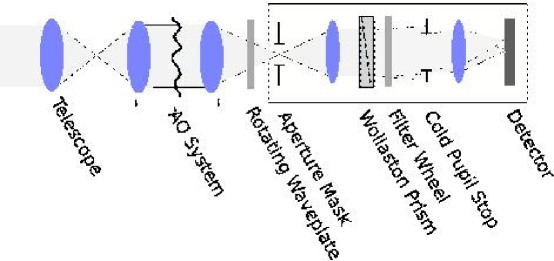
Figure 1.— A simplified schematic of the IRCAL polarimeter, not to scale but indicating the order of the various optical components. The box represents IRCAL’s vacuum dewar. Labeled in bold are the polarimetry components added to the original AO system and camera: the rotating waveplate, the aperture mask, and the Wollaston prism mounted in the first of IRCAL’s two internal filter wheels. The Wollaston prism splits the collimated beam, forming on the detector two simultaneous images with perpendicular polarizations. Rotation of the waveplate modulates the intensity of the two images, allowing the measurement of Stokes $Q$ and $U$.

3.1. General Design Considerations

A Wollaston prism (Wollaston, 1820) deflects perpendicular polarizations oppositely, with the angle of each output beam approximately equal to

$$\delta\simeq\Delta{n}\tan\alpha$$

where $\alpha$ is the prism angle and $\Delta{n}$ is the birefringence. If such a prism is placed conjugate to the telescope pupil, it will split the incident beam to create two polarized images on the final detector plane. The Lagrange invariant implies that each of these images will have an apparent sky-projected deflection of

$$\delta_{\mathrm{projected}}\simeq\left(\frac{D_{\mathrm{pupil}}}{D_{\mathrm{tel}}}\right)\Delta{n}\tan\alpha$$ (1)

where $D_{\mathrm{pupil}}$ and $D_{\mathrm{tel}}$ are the pupil image and telescope diameters (5 mm and 3 m respectively in our case). The polarimetric field of view is maximized if the total separation $2\delta_{\mathrm{projected}}$ is half the detector’s total field of view. For IRCAL, this field of view is 19.4″, implying an optimal $\delta_{\mathrm{projected}}\sim 4.9^{\prime\prime}$. Thus once we have chosen our material (and therefore $\Delta{n}$), equation 1 may be solved for the necessary prism angle $\alpha$.

Oliva (1997) proposed using a wedged double Wollaston for simultaneous measurement of all four polarization states, and thus simultaneous extraction of Stokes $Q$ and $U$. However, this approach requires dividing the pupil in half, resulting in a loss of half the angular resolving power of the system, so the wedged double Wollaston is not an optimal solution for high resolution imaging. The pupil division also means that the $Q$ and $U$ beams see different portions of the atmosphere and will have PSFs at least as divergent as if they were non-simultaneous. Furthermore, obtaining a given signal-to-noise level in both $Q$ and $U$ requires just as much total exposure time as in a regular dual-beam polarimeter. We therefore chose to develop a classical single-Wollaston polarimeter.

We also chose to use a conventional rotating half-wave plate as the polarization modulator, instead of alternatives such as liquid crystal variable retarders (LCVRs) or ferroelectric liquid crystals. Ferroelectric liquid crystals are unsuitable given their too-fast modulation compared to typical infrared detector readout times. LCVRs provide spectacular levels of precision in solar polarimetry, but are generally not achromatic, are difficult to obtain for wavelengths beyond 1.8$\mathrm{\ \mu{m}}$, and have birefringence that is temperature-dependent. In contrast, half-wave plates are available with excellent achromaticity and low sensitivity to temperature variations. Since we desired a single modulator for the entire 1-2.5$\mathrm{\ \mu{m}}$ band, we use an achromatic waveplate as our modulator. Figure 1 shows the overall layout of the IRCAL polarimeter including the above-mentioned components.

3.2. Choice of material for the Wollaston prism

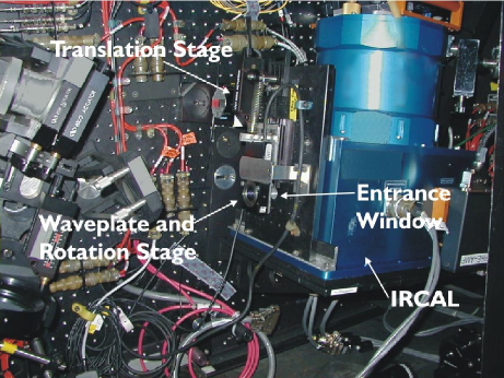
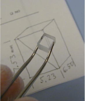
Figure 2.— Left: The IRCAL dewar mounted on the Lick AO optical bench at the Cassegrain focus of the 3-m Shane telescope, highlighting the waveplate mechanisms. A rotation stage allows modulation of the polarization using the waveplate, and a linear translation stage allows inserting/removing the waveplate from the beam. Right: Our YLF Wollaston prism, manufactured by Onyx Optics of Dublin, CA. This prism has been installed in one of IRCAL’s two cryogenic filter wheels since March 2002.

Oliva et al. (1997) provides an overview of candidate birefringent materials for infrared Wollaston prisms. We present in Appendix A an updated list of such materials, along with recent references for their optical properties.

For an imaging polarimeter, it is important to choose a material whose birefringence $\Delta{n}$ does not vary much within each operating bandpass. A wavelength-dependent $\Delta{n}$ causes different beam deflections for each wavelength within a bandpass, elongating the final image. Minimizing this effect, called “lateral chromatism”, is particularly important for a high contrast polarimeter: not only does lateral chromatism decrease angular resolution, it can greatly degrade PSF subtraction quality by oppositely distorting the two polarizations’ PSFs. Lateral chromatism may be quantified over a given wavelength range $\lambda_{1}<\lambda<\lambda_{2}$ by Oliva’s parameter

$$V_{\Delta{n}}=\frac{\Delta{n_{(\lambda_{1}+\lambda_{2})/2}}}{\Delta{n_{\lambda_{1}}}-\Delta{n_{\lambda_{2}}}}$$

This parameter is the birefringent analogue to the Abbe number $V$, which measures dispersion in optical materials. High values of $V_{\Delta{n}}$ correspond to low amounts of birefringent dispersion. The image elongation over the range $\lambda_{1}-\lambda_{2}$ will be $\epsilon=\delta/V_{\Delta{n}}$. By selecting a material to maximize $V_{\Delta{n}}$, we can minimize blurring due to lateral chromatism.

We chose the unaxial birefringent material YLF (yttrium lithium fluoride, LiYF₄, pronounced “yilf” by its users in the laser industry) because its $\Delta{n}$ is remarkably constant with wavelength, causing negligible lateral chromatism. Typically, $V_{\Delta{n}}>100$ is considered good, corresponding to chromatic elongation less than 0.05″ for IRCAL, better than the diffraction limit. YLF exceeds this (spectacularly at $H$, with $V_{\Delta{n}}=1290$) and is readily available due to its widespread use in the laser industry. Its refractive index, 1.45, is similar to that of standard optical components, simplifying the optical design and manufacturing, and its birefringence, $\Delta{n}$ = 0.022, allows the necessary beam divergence to be obtained with an reasonable thickness of YLF, roughly 4 mm.

Three similar Wollaston prisms were fabricated by Onyx Optics of Dublin, CA and were received at Berkeley in March 2002 (Figure 2). The pieces were joined using optical contacting and both exterior surfaces received a 1-2.5$\mathrm{\ \mu{m}}$ antireflection coating. The 30° prism angle produces a beam divergence of 1.45°, giving a sky-projected separation of 8.6″ between the two beams (close to the optimal value of half the field of view). All three prisms performed as expected in laboratory tests. Two of the prisms exhibited minor surface defects, so we selected the third for astronomical use. That Wollaston was installed in one of IRCAL’s internal filter wheels, in collimated space just before the cold pupil.

A concern with any birefringent material is that the differing optic axes will have different thermal expansion coefficients. For Wollaston prisms constructed by bonding two surfaces with perpendicular axes, temperature changes create stress between the two faces. YLF has fairly similar expansion coefficients of $5\times 10^{-6}\ \mathrm{K}^{-1}$ parallel and $8\times 10^{-6}\ \mathrm{K}^{-1}$ perpendicular to the fast axis. Our prism has tolerated repeated thermal cycling to liquid nitrogen temperatures with no ill effects apparent after five years.

One caveat about YLF is it is relatively expensive and can be hard to obtain in large sizes, such as needed for Wollastons on 8-10 m telescopes. The greater angular resolution of large telescopes places a stringent constraint on lateral chromatism, requiring high $V_{\Delta{n}}$ materials like YLF for diffraction-limited performance. However, a large YLF Wollaston was recently fabricated for the Subaru Telescope (Hodapp et al., 2007), demonstrating that the crystal fabrication challenges can be overcome.

3.3. Waveplate and Aperture Mask

We obtained an achromatic waveplate from Karl Lambrecht Corp., fabricated from MgF₂ and crystal quartz. The waveplate is optimized for 1-1.6$\mathrm{\ \mu{m}}$, and provides $0.500\pm 0.005$ waves of retardance over that range. At longer wavelengths, the retardance differs from half a wave by about 0.05 waves averaged across the $K_{s}$ band. As a result the polarizing efficiency of the instrument is degraded slightly at long wavelengths, as discussed below in §4. The waveplate is installed in a Newport PR50 rotation stage, itself mounted on a translation stage for insertion into the optical path (Figure 2). For practical reasons, the waveplate is located at the entrance window to IRCAL. Ideally, it should have been placed as far upstream as possible, since modulation allows any instrumental polarization from post-modulator optics to be separated from the astronomical signal, but given the constraints of the AO bench that was not feasible. As a result, polarizing optics before the modulator, such as tilted mirrors and the dichroic beamsplitter, introduce a nonzero instrumental polarization.

To prevent overlap of the two polarized images, we installed in IRCAL’s cold aperture wheel a rectangular mask corresponding to half the field of view, essentially a $9\arcsec$ wide slit. As fabricated, the mask is slightly oversized, resulting in an 0.4″ (6 pixels or 240$\mathrm{\ \mu{m}}$) beam overlap in the middle of the detector. This overlap region is discarded during data reduction.

3.4. Limitations and Imperfections

The IRCAL polarimeter’s performance is limited by several factors in its design and construction. For instance, errors in flat fielding prevent completely accurate subtraction of the two polarizations. Modulation reduces the impact of this, but cannot eliminate the problem entirely. Even though both polarizations are alternately measured on both sides of the detector, the images must be shifted to register them before subtraction, which depends on accurate flat fielding to maximize the cancellation of starlight.

A second factor that limits real-world polarimeters is registration and shifting errors (e.g. Apai et al., 2004). IRCAL’s coarse pixel sampling (which only Nyquist-samples the PSF at wavelengths $>2\mathrm{\ \mu{m}}$) exacerbates this. The undersampled nature of $J$- and $H$-band data limits the precision possible in registration and introduces aliasing that compromises image subtraction. Even were the sampling improved, accurately registering images would still be challenging, particularly for deep exposures saturated on the central core.

The placement of the Wollaston prism in a filter wheel before the cold pupil results in the two polarized beams already having diverged by the time they reach that pupil stop. This “pupil shear” causes each channel to have a slightly different effective pupil and significantly increases the non-common-path aberrations between the two beams. Traced backward through the telescope and onto the sky, each channel sees a slightly different column of partially-corrected atmosphere, displaced from the other by $\sim 5\%$ of the pupil diameter. This results in non-common-path atmospheric wavefront errors, which cannot be compensated for by waveplate modulation. It would have been much better to place the Wollaston after the cold pupil, but the layout of the existing filter wheels didn’t allow this.

IRCAL’s aperture mask wheel is not a precision mechanism. Its positioning has low repeatability, and it occasionaly shifts unpredictably (apparently as a result of electrical crosstalk from one of the other wheel mechanisms). Shifts in the aperture mask change the field of view and flat field for the observations. The filter wheel containing the Wollaston is less sensitive, but slight offsets from night to night change the relative position of the two polarized images, which the data reduction pipeline must deal with.

Compared to these factors, any imperfections in the polarimetry optics themselves, and/or the finite precision of the waveplate rotation (0.1°), are entirely negligible. Wollaston prisms frequently achieve extinction ratios better than $10^{-5}$; at this time, we cannot more precisely quantify the performance of our prism but believe that its extinction ratio and polarizing efficiency are excellent.

4. Commissioning Tests

The prism was installed into IRCAL during 2002 March, and had first light on 2002 March 29 UT. Observations then and on subsequent nights have allowed us to quantify the performance of the system.

The polarimetry optics have negligible effect on the achieved AO image quality. They do contribute additional non-common-path wavefront error between the science detector and wavefront sensor (including about 1.3 mm of focus and 85 nm RMS of other aberrations, principally astigmatism) but by applying appropriate offsets to the deformable mirror, we can fully compensate for these aberrations. This results in internal Strehl ratios of $0.92\pm 0.02$, essentially identical to performance without the polarimetry optics. The resulting orthogonal polarized PSFs appear very similar but not perfectly identical, confirming the presence of small non-common-path wavefront errors between the two polarizations.

We observed the Lick AO system’s internal calibration source to determine the throughput of the Wollaston prism and waveplate, including both reflective losses and absorption. At longer wavelengths, YLF becomes more transparent, but the waveplate’s antireflection coating performs less well. This results in a net transmission through both optics of $92.3\pm 0.3\%$ at $J$ and $H$, decreasing to $88.5\pm 0.5\%$ at $K_{s}$.

To calibrate the polarizing efficiency, we placed in front of the AO calibration source a 1-2$\mathrm{\ \mu{m}}$ IR Polaroid from Edmund Scientific, and observed its apparent brightness as a function of waveplate angle, for each of $J$, $H$, and $K_{s}$. We fit a model to these data using the Levenberg-Marquardt least-squares method to extract the polarizing efficiency. The polarizing efficiency measured in this way is $1.00\pm 0.005$ for $J$ and $H$, and $0.95\pm 0.01$ for $K_{s}$ band. This decreased polarizing efficiency at $K_{s}$ is due entirely to the waveplate’s retardance differing slightly from half a wave at wavelengths beyond 1.8 µm.

4.1. Instrumental Polarization

Instrumental polarization of some degree is found in all optical systems, particularly those that depart from circular symmetry, such as by having oblique reflections. The Lick AO optical path involves many such reflections, and thus moderate instrumental polarization is expected. Accurately modeling instrumental polarization is challenging, as oxide layers on mirrors and other subtle imperfections can play substantial roles (Keller, 2002). For very high contrast applications, the polarizing effects of thin metal films must be considered (Born & Wolf, 1959; Breckinridge & Oppenheimer, 2004).

We observed unpolarized standard stars (Gehrels, 1974; Ageorges & Walsh, 1999) to calibrate instrumental polarization. We measured the apparent polarization of each standard via aperture photometry on the reduced data, and interpreted the apparent polarizations as the amount of instrumental polarization. For all wavelengths, the derived instrumental polarizations are around 2.5% in the $-Q$ direction. Due to the Cassegrain configuration, these values are extremely stable with time, changing $<0.1\%$ in observations of standard stars more than a year apart. Based on comparison of these measurements to a Mueller matrix model of the optical train, the instrumental polarization appears to be primarily caused by the dichroic that separates the visible wavefront-sensing and IR science channels. This large contribution is unsurprising for a complex multilayer optic at oblique incidence. We did not attempt to measure circular instrumental polarization or crosstalk between circular and linear polarizations.

The optimal method to remove instrumental polarization depends on the science goals. We adopt an iterative optimizing subtraction process that simultaneously removes linear instrumental and interstellar polarization, described in §6.1.

4.2. Pixel Scale

Lloyd et al. (2000) previously measured IRCAL’s pixel scale as $0.0756\arcsec\pm 0.0002$ pixel^-1. Subsequent observations have allowed a refined measurement, revealing slightly different plate scales in R.A. and Dec. This indicates that IRCAL is anamorphic, a result not unexpected given that its internal off-axis parabolic mirrors are not of unit magnification.

To quantify the anamorphism, we obtained LGS AO observations of the core of the globular cluster M 53. We extracted point source coordinates using the Starfinder IDL package, and compared them to coordinates derived from HST WFPC2 imaging of the same cluster (Piotto et al., 2002). We simultaneously fit the displacement, rotation, shear, and x- and y-magnification between the two datasets using the MPFIT Levenberg-Marquardt nonlinear least squares optimizer. This analysis yielded plate scales of $0.0754\arcsec$ pixel^-1 in R.A. and $0.0780\arcsec$ pixel^-1 in Dec., with statistical error $\pm 0.0005\arcsec$ pixel^-1. The detector’s axes are orthogonal within our 0.5° measurement uncertainty.

To correct the anamorphism, we developed an IDL routine ircal_dewarp, based on Keck’s nirc2warp by Antonin Bouchez. This routine transforms a distorted input image onto a uniform 0.040″ grid via two-dimensional cubic spline interpolation.

To assess the performance of this correction, and to measure any shifts in the absolute orientation of IRCAL over time, we routinely observe binary stars drawn from the Suggested Calibration Targets list of the Washington Double Stars (WDS) Orbits Catalog (Hartkopf et al., 2001). The observed binary separations are compared to values computed from the WDS orbital elements. Because the WDS Orbits Catalog is itself imperfect (most of the binaries with suitable separations and brightnesses have orbits graded 4 or 5, the lowest grades) some amount of discrepancy is expected. Since many entries in the WDS do not contain estimated uncertainties, we make no attempt here to separate out these two effects. A conservative estimate is that the pixel scale in post-anamorphism-correction IRCAL images is uncertain by no more than $\sim$2.5% in linear size, and by $\sim$1.0° in position angle.

The cubic spline interpolation employed is a good approximation to the theoretically optimum sinc interpolation, but not perfect, particularly given the non-Nyquist-sampled nature of short-wavelength IRCAL data. “Ringing” artifacts (the “Gibbs phenomenon”) are sometimes seen near stellar PSF peaks in dewarped images. It is worth noting that the ircal_dewarp routine is not strictly flux conserving, nor does it account for the small higher-order distortions present in IRCAL (M. P. Fitzgerald, private communication). Attempting to characterize and compensate for these effects, either through heuristic algorithms such as Drizzle (Fruchter & Hook, 2002) or through more formally correct Fourier interlacing methods (Bracewell 1978, Lauer 1999), is beyond the scope of this paper.

5. Observing Techniques and Astronomical Calibration

5.1. Observing Procedure

Our standard observing procedure is as follows: Once the target has been acquired, the observer configures settings such as filter and exposure time. The camera’s software automatically rotates the waveplate and integrates at each position. We use eight distinct waveplate positions: 0, 22.5, 45, 67.5, 90, 112.5, 135, and 157°. This provides four redundant measurements for each of Stokes $Q$ and $U$, reducing instrumental systematics (Kuhn et al., 2001; Patat & Romaniello, 2006). To obtain the necessary high dynamic range, for most targets it is necessary to combine both short and long exposures, typically between 0.5 and 90 s, depending on source magnitude. Small dithers after each set of eight exposures are used to reduce flat field effects and/or increase field of view.

5.2. Flat fielding

As flat-fielding errors are expected to be a major contributor to systematic limits on the detection of faint polarized circumstellar material, several methods were pursued for flat-fielding the polarimeter. The IRCAL aperture mask and filter wheel positioning mechanisms have frustratingly poor repeatability. Because of this, the aperture mask position can only be approximately reproduced from night to night (typically within 5-10 pixels), so it is necessary to take flats again every night. Some authors have advocated computing flat field calibrations using observations of extended sources such as planets (Kuhn et al., 1991), but such targets are not always visible. We instead opt for the more traditional sky as flat calibrator.

Because the twilight sky is itself highly polarized, it is far from ideal for flat fielding a polarimeter. Dome flat screens are typically only slightly better. To get around this problem, polarized sky or dome exposures taken with different waveplate angles are averaged to make “pseudo-unpolarized” flat frames. This method only works perfectly if the sky brightness and polarization are constant, a requirement notably not satisfied during twilight (see Cronin et al. (2006) for discussion of sky polarization during twilight and its variation with time). IRCAL’s small pixel scale allows it to take unsaturated exposures on the daylit sky hours before sunset, at which point the sky polarization is more stable.

From each night’s set of “pseudo-unpolarized” frames we compute one master median flat per wavelength, which we use for all waveplate angles. Errors in the final master flats are estimated to be a few parts in a thousand. Some authors have reported slight benefits from using a flat frame computed individually for each waveplate angle (Ageorges & Walsh, 1999). We did not investigate that approach in detail, but note that it may offer future potential for improvement.

The nightly flat fields are also used to measure the location on the detector of the two polarized subimages, using a Hough-transform edge detection algorithm to find the edges of the illuminated fields of view. The detected masks are undersized by 5 pixels to avoid light scattered from the aperture mask’s edges.

5.3. Sky Subtraction

At night the infrared sky background is primarily unpolarized, vibrationally excited emission from atmospheric molecules. In dual-channel differential polarimetry, this unpolarized background will subtract out of the $Q$ and $U$ images. Thus there would be no need to worry about sky subtraction, if our sole concern was the polarized images. However, since we also want to measure total intensity for each target, we perform the usual sky subtraction. We subtract a distinct sky frame for each waveplate angle, obtained either from separate sky frames or as a median of the dithered science frames with that angle. This process also allows for the subtraction of any polarized sky light such as scattered moonlight, but as mentioned above, this is usually negligible.

5.4. Polarization Angle Calibration

The Stokes reference frame must be oriented relative to some known reference angle. (Equivalently, we must determine the rotational zeropoint for the waveplate mechanism.) We do this using the twilight sky, which is strongly linearly polarized perpendicular to the direction pointing toward the sun (Cronin et al., 2006). Using the sky as a calibrator allows us to use all pixels of the detector and thus rapidly obtain high signal to noise. In practice, the same data are used for flat fielding the detector and for calibrating the position angle.

5.5. Photometric Calibration

Photometric standards (e.g. Persson et al., 1998; Hawarden et al., 2001) are observed using the same procedure as science targets. After the standard polarimetry reduction (described in §6), we measure their fluxes within a 7″ diameter aperture, plus encircled energy curves for aperture correction. Adaptive optics photometry is a notoriously problematic area due to PSF variability (see Fitzgerald & Graham, 2006; Sheehy et al., 2006). Changes in sky conditions and guide star brightness inevitably cause wavefront correction to vary between science target and calibration source, causing photometric errors as the encircled energy curve changes. We expect an uncertainty of 5-10% in the resulting photometry in typical conditions.

6. The IRCAL Polarimetry Data Reduction Pipeline

Data reduction for imaging polarimetry has been discussed before by a number of authors (Gledhill et al., 1991; Wolstencroft et al., 1995; Kuhn et al., 2001; Potter, 2003a; Patat & Romaniello, 2006). The reduction algorithms for IRCAL build on these earlier works but also feature a number of elements specific to IRCAL. We describe here the data reduction process in detail, in the hope of sharing lessons from IRCAL with other aspiring differential polarimetrists. Furthermore, this is an appropriate setting to air dirty laundry: that is, to highlight what doesn’t work about IRCAL polarimetry as well as what does, and what aspects should be improved in future designs, such as the planned polarimetry mode of the Gemini Planet Imager.

6.1. General Considerations

Our fundamental goal is to use polarimetry to cancel out the unpolarized stellar PSF and reveal faint circumstellar material. In practice, complications such as instrumental and interstellar polarization mean that the star’s PSF is not truly unpolarized. For distant or young and embedded sources, interstellar polarization can be substantial, at a level of a few percent. While it is possible to remove interstellar polarization based on observations of nearby stars (Heiles, 2000), this is fraught with uncertainties. Not least of these is the assumption that interstellar polarizations vary in a predictable and uniform way between stars– an assumption unlikely to be satisfied in the clumpy, dusty environments of young stars. Is there a better approach?

We can instead allow the net polarization of the star (arising from both interstellar and instrumental polarization) to be a free parameter that we solve for. We do this by finding the scaling coefficients that minimize residual starlight in $|Q|$ and $|U|$, following the approach used by Potter (2003a). This method relies on the assumption that the total flux is dominated by inherently unpolarized light, so that any net polarization seen in the data is the result of instrumental or interstellar polarization. For our science targets, this is generally an good approximation, since scattered light is no more than a few percent of the total.

This approach is robust even in the presence of scattered light. For a symmetric distribution of dust around a star, the polarization position angle varies around the disk and the total net polarization in a large aperture cancels to zero. For inclined or nonaxisymmetric dust distributions, that cancellation begins to break down and can introduce a systematic bias to underestimate the true degree of polarization. In an extreme case, a 100% linearly polarized source would not be measurable with this technique at all. But as mentioned above, we restrict our efforts to the detection of spatially varying polarization from resolved dust. For such systems, the uncertainty resulting from this scaling process will be negligible compared to other factors, such as the biasing effect of the PSF halo in Stokes $I$.

With that goal in mind—the detection of faint spatially resolved polarization from extended circumstellar dust, and not the precise measurement of total polarization—an IDL data reduction pipeline for IRCAL polarimetry data has been developed. This software is available online and automatically handles the reduction, calibration, and analysis of IRCAL polarimetry data. Minimal user intervention is required to produce first-pass science reductions, though extensive options exist for overriding or fine-tuning the pipeline’s behavior.

6.2. Initial Reduction

Images are first dark-subtracted, then divided by the polarization mode flat field. Sky subtraction is performed, as described above. Bad pixels are identified and removed, using the combination of a mask indicating known permanently-bad pixels and the NIRSPEC fixpix iterative bad pixel cleaning routine developed by Tom Murphy. At this point, the images are relatively clean, and can be corrected for anamorphism using the ircal_dewarp routine (§4.2).

Saturated pixels and/or pixels above the detector’s linear regime are identified by comparison with a threshold value of 280,000 electrons pixel^-1. The saturated pixel lists for the two polarized subimages are merged to ensure that if any pixel is marked as saturated, its corresponding pixel in the other polarization is also marked as saturated. Without this step, polarization artifacts would be induced later during image subtraction.

6.3. Registration

Accurate registration to a fraction of a pixel is required to extract polarized signals very close to a star. Apai et al. (2004) found that for AO polarimetry at the Very Large Telescope, random shifts of 0.2-0.5 pixel (5-14 mas) distort the polarized signal of the inner arcsecond, and shifts of 1 pixel completely disrupt it. Long exposure images, which probe polarization on slightly larger scales, are more robust against misalignments. Apai et al. used a “two-level Gaussian fitting procedure” to register their data, while Potter (2003a) used an iterative shift-and-subtract process to empirically find the shift for each image that gave the lowest residuals. For IRCAL we use Fourier cross-correlation to subpixel precision. Which of these techniques is best will vary depending on instrument and observational conditions.

The first step in image registration is to determine the offset between the two polarized subimages on the detector, which varies slightly from night to night due to imprecision in the filter wheel rotation. To measure this, the full stack of images is summed, and the resulting left- and right-hand subimages are cross-correlated to find their displacement.

The individual images are then registered via cross-correlation, fit by Gaussians to subpixel precision. Only the left-hand subimages are correlated, with the same shifts (plus the beam displacement) assumed correct for the right hand field. If necessary, manual intervention is possible to tweak the automatic registration.

An important caveat about IRCAL polarimetry is that the images are only Nyquist sampled at $K_{s}$. At shorter wavelengths, high spatial frequency PSF structure will alias to lower spatial frequencies, biasing the correlations and derived shifts in an unpredictable and time-variable manner. In the absence of a priori PSF knowledge, this imposes a fundamental limit on our ability to accurately register these images. Furthermore, the long exposures necessary to detect faint circumstellar dust are frequently saturated on the central star, which limits registration accuracy even more. Cross-correlation still works to some extent in this case, using the diffraction spikes and other outer PSF structure, which is why we chose that approach for the IRCAL pipeline. The highest accuracy polarimetric image registration may require the use of “satellite PSF” techniques developed for coronagraphic observations (Marois et al., 2006; Sivaramakrishnan & Oppenheimer, 2006).

6.4. Mosaicing

All the subimages for a given polarization are then mosaiced together, combining different exposure times via a weighted average. Subpixel shifting is done by Fourier interpolation. A separate mosaiced image $M_{i}$ is produced for each of four polarization angles: $M_{0},M_{45},M_{22.5}$, and $M_{67.5}$. These mosaics combine polarized subimages from both sides of the detector, and images from the redundant waveplate settings 90, 135, 112.5 and 167.5 are summed with their counterparts (i.e. images taken with the waveplate at 90$\arcdeg$ are mosaiced in with those taken at 0, and so on.)

The resulting mosaics are then scaled to minimize their subtracted residuals $Q$ and $U$, according to

$$Q = M_{0}-\alpha M_{45}+\beta$$

$$U = M_{22.5}-\gamma M_{67.5}+\delta$$

$$I = \left(M_{0}+\alpha M_{45}+M_{22.5}+\gamma M_{67.5}\right)/2.$$

The coefficients for minimizing the total power in $|Q|$ and $|U|$ are determined by IDL’s Powell nonlinear optimization routine. Typical values for $\alpha$ and $\gamma$, the scaling factors that remove the net polarization of the targets, are within a few percent of unity. The $\beta$ and $\delta$ factors correct for any residuals in the sky background levels, and are always small.

This order of operations—mosaicing the images, then performing the scaled subtraction—is by no means the only way to do things. One can also first difference the images and then mosaic the subtracted frames, or there are also reduction algorithms that rely upon ratios rather than differences of the two channels (see Tinbergen, 1996). We chose the mosaic-then-subtract approach because it offered greater flexibility for dealing with missing frames from AO system dropouts or moments of bad seeing, but the merits of the various algorithms should be reevaluated for future instruments.

The polarized intensity $P$ is computed from $Q$ and $U$ in the usual manner, $P=\sqrt{Q^{2}+U^{2}}$. If absolute accuracy in $P$ were our goal, we would need at this point to remove the bias introduced into $P$ by its positive definite nature, by following one of the the standard statistical debiasing algorithms (Wardle & Kronberg, 1974; Simmons & Stewart, 1985; Stewart, 1991). But we skip this step for two reasons. First, these corrections are important primarily when the signal to noise ratio is low ($P/\sigma_{P}\lesssim 2$), and we focus our analysis only on pixels with strong detections of polarization ($P/\sigma_{P}>3$). Much more importantly, for AO data the bias in degree of polarization $P/I$ from the uncorrected PSF halo in Stokes $I$ will be far larger than this statistical bias. Recall our goal is not to make absolute polarization measurements; when attempting to use polarimetry to detect fainter signals hidden in the speckled PSF halo, it is simply infeasible to make absolute measurements of $P/I$ and so we do not try.

Along with the mosaics, we generate exposure maps and per-pixel empirical uncertainty images for $I$, $Q$ and $U$, computed from the standard deviation of double-differenced pairs of input frames. Computing the per-pixel uncertainty based on unsubtracted or single-subtracted images would not provide an accurate assessment of the speckle-noise-reduced characteristics of the final Stokes images. During the course of our AO polarimetry survey of Herbig Ae/Be stars, these uncertainty maps proved very valuable in assessing the significance of faint signals.

6.5. Final Steps

The last steps in reduction are updating the World Coordinate System header, and flux calibration in Jy arcsec^-2 based on the closest-in-time photometric standard. The final images are stored as multi-extension FITS files containing the Stokes data cubes, exposure maps, and uncertainty images.

These data may be visualized using several IDL plotting routines, or interactively explored using a version of the atv image display tool (Barth, 2001) modified to accept Stokes data cubes and overplot polarization vectors. This code is available from the author’s web site.

7. Achieved Performance

7.1. Contrast Enhancement

In practice the IRCAL polarimeter and data reduction pipeline remove 98-99% of unpolarized starlight, greatly attenuating the background against which scattered light must be detected (Figure 3). The exact level of performance varies with conditions.

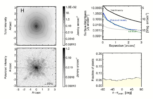
Figure 3.— $H$ band imaging polarimetry of the unpolarized standard HD 18803, demonstrating the cancellation of unpolarized starlight. Left: Total and polarized intensity. The display scale for polarized intensity is reduced by 100 compared with total intensity. Right, top: Radial profiles showing total and polarized intensity and the minimum theoretical noise floor for $P$ based on photon statistics and read noise. As a rough estimate of the light-suppression capabilities of the polarimeter, the thin dashed line shows a copy of the $I$ profile that has been multiplicatively scaled by $0.015$ to match the $P$ profile. In other words, the polarimeter rejects 98.5% of unpolarized starlight for this observation. Right, bottom: A histogram of polarization position vectors relative to the expected centrosymmetric pattern that indicates circumstellar dust (see §7.2). The uniform distribution seen here is the expected null result for an unpolarized star.

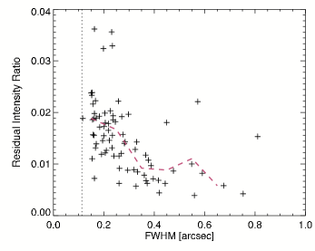
Figure 4.— The fraction of residual starlight not suppressed by polarimetry (measured as the ratio of apparent polarized intensity over total starlight) plotted versus PSF full-width at half maximum (FWHM). The dashed line shows the average suppression ratio in each 0.1″ wide bin, and the vertical dotted line shows the minimum diffraction-limited FWHM. Higher ratios mean more unpolarized starlight is leaking through into the final polarized intensity images. The suppression of unpolarized starlight is best for observations with large FWHM, and conversely worst when the AO correction provides the best FWHMs. This surprising result indicates that high spatial frequencies in the PSF contribute strongly to the subtraction residuals, suggesting that registration and aliasing rather than flat fielding errors set the greatest limits on performance for our polarimeter.

Outside of $\sim$1″, we typically reach a noise floor $P_{noise}$ set by photon and read noise. Inside that radius, instrumental systematics raise the polarized surface brightness background above the theoretical noise floor. The precise transition between photon-noise-limited and systematic-limited depends on factors including source brightness and seeing; for some of our targets the transition occurs inside 1″ (though rarely inside 0.7″) and for some it’s further out. This performance is similar to that achieved by Potter (2003a) with the Hokupa’a polarimeter.

Like speckle noise, the systematic noise floor is not Gaussian and does not improve with time as $\sqrt{t}$. Additional integration increases the sensitivity at small radii only slightly if at all, similar to the behavior of semi-static speckles in conventional AO imaging (e.g. Racine et al., 1999; Aime & Soummer, 2004; Hinkley et al., 2007). But we stress here that the polarimetric noise floor is not merely semi-static speckles rearing their ugly heads: a perfect polarimeter would completely reject any static speckles, no matter how aberrated the $I$ PSF. It is imperfections in the polarimeter that allow a fraction of those speckles to bleed from $I$ into $P$ and ultimately limit our sensitivity.

Many factors contribute to this imperfect subtraction of images. Is it possible to disentangle which of these—flat fielding error, pupil shear, registration error, and so on—is dominant? In practice, for IRCAL it has proven difficult to quantitatively assess the relative importance of the various error terms. In part this is because of the instrument’s history. It was a mode retrofitted into the camera at the telescope, and it never underwent any laboratory tests with high-quality polarized calibration sources. More fundamentally, the various terms in the error budget all have similar functional forms, $P_{noise}\propto I$. Flat field errors, registration errors, pupil shear, all introduce noise proportional to total intensity, rendering it hard to empirically disentangle the magnitude of each individual effect.

We thus present only a partial resolution to this issue. For each target observed during our Herbig Ae/Be survey, we estimated the polarized noise floor as a fraction of total intensity, by computing the median ratio of the radial profiles of $P$ and $I$ between 0.2″ and 2.0.″ In Figure 4, we plot this ratio against the PSF FWHM, a measure of wavefront quality. The result is striking: as AO performance improves (i.e. the FWHM becomes smaller), on average a larger fraction of light “leaks through” the polarimeter. Better seeing and higher Strehl PSFs perversely result in slightly worse PSF subtractions!

From this we conclude that the subtracton residuals increase when the PSF has more power at high spatial frequencies. Errors in flat fielding would not cause this; such errors should be a simple multiplicative factor on the PSF, regardless of PSF shape. On the other hand, errors from PSF registration, aliasing, and numerical interpolation will grow as high spatial frequency power increases, particularly for an undersampled detector such as IRCAL’s. Registration errors of saturated images will also contribute to this problem. Long exposures are needed to detect faint outer nebulae, and in such data the core of the PSF will be saturated and thus unusable for registration. In conditions with better seeing, saturation will occur earlier, contributing to the observed degradation. Thus for IRCAL it appears that image registration and aliasing are a more significant limitation than flat fielding.

7.2. Detection of polarized light in reduced images

In some cases polarized structures are immediately visible in reduced images, but more often we face the task of detecting faint polarizations at low signal to noise. How may we best decide whether a given data set shows robust evidence for detected polarization or not?

Merely looking by eye at polarization images is an ineffective way to approach these data. Polarization is fundamentally a vector quantity, and examining only one of $Q$ or $U$ at a time does not take full advantage of that richness. Hunting for a faint signal in $P$ is also not the best approach: $P$ incorporates both Stokes $Q$ and $U$, but its positive definite nature biases it so any noise whatsoever results in a nonzero, positive value, which swamps faint polarized signals. Numerical fits should be done directly on the $Q$ and $U$ images, and only transformed to $P$ afterwards if necessary.

Luckily, light scattered from circumstellar dust has a distinct signature we can search for. This characteristic may be visualized either as the so-called “butterfly” pattern in the $Q$ and $U$ images, or as a “centrosymmetric” circular pattern of polarization vectors arranged circumferentially around the central source. Apai et al. (2004) fit a sinusoid to the butterfly pattern in $Q$ and $U$ images to detected scattered light to within 0.1″ of TW Hya. A closely related technique uses instead the polarization position angle $\theta$. The position angles for centrosymmetric scattering are given by

$$\theta_{centro}(x,y)=\arctan\left(\frac{y-y_{\ast}}{x-x_{\ast}}\right),$$

where $(x_{\ast},y_{\ast})$ is the central star’s location. By comparing the observed position angle $\theta_{obs}(x,y)$ with the expected position angle $\theta_{centro}$, we can sensitively discriminate dust-scattered light from other contaminants such as residual speckle noise or registration errors. A key advantage is that the position angle $\theta_{obs}$ is formed from the ratio of $Q$ and $U$, and hence is less sensitive to flat fielding errors than either of those quantities alone (Potter, 2003a).

See Figure 5 for a demonstration of using this method to detect a very faint polarized signal from a disk around the Herbig Ae star HD 141569. Located at 99 pc, this young star has a circumstellar disk believed to be transitioning from optically thick to optically thin, possibly due to the clearing effects of unseen planets. Based on prior coronagraphic observations (Weinberger et al., 1999; Clampin et al., 2003; Boccaletti et al., 2003), the disk’s $H$-band surface brightness is 16-17 mag. arcsec^-2 between 1-2″radii, compared to a stellar magnitude of $H=6.8$. We observed HD 141569 on 2003 June 17 for 1600 s total, as part of a large survey of dust around Herbig Ae/Be stars (Perrin et al,̇ in preparation). The disk’s structure is not at all apparent in the $I$ or $P$ images. However, if we plot a histogram of the position angles for pixels which have polarized S/N $>3$, we find they are predominantly close to the expected centrosymmetric angles (seen in the lower right panel in Figure 5). The observed polarization signal is strongest near the location of the bright outer ring previously seen by NICMOS and ACS. While this observation only marginally detects this disk and does not reveal its structure clearly, to our knowledge this is the first non-coronagraphic detection of HD 141569’s disk in the near-IR. This demonstrates that centrosymmetry histograms can be used to sensitively detect extremely faint polarized signals which might otherwise be missed.

Recently, Schmid et al. (2006) have advocated the use of “radial Stokes parameters” as an alternative technique that combines aspects of both the butterfly and centrosymmetry methods. In this approach the Stokes vectors are transformed according to

$$Q_{r} = +Q\cos 2\phi+U\sin 2\phi$$

$$U_{r} = -Q\sin 2\phi+U\cos 2\phi$$

where $\phi$ is the position angle measured from the central source. $Q_{r}$ is then a measure of the polarization’s centrosymmetry. The use of these quantities for polarimetric analysis deserves further study.

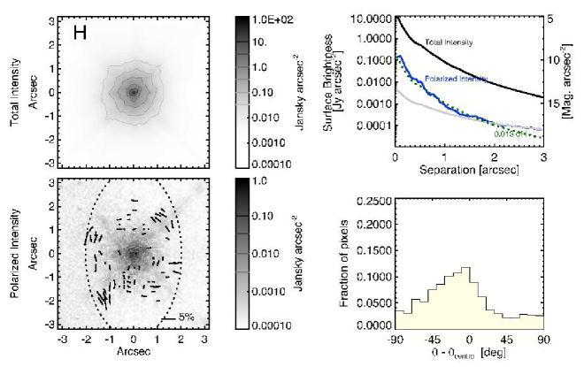
Figure 5.— $H$ band polarimetry of a very faint signal: the circumstellar disk of the Herbig Ae star HD 141569. See the caption of Figure 3 for a description of the various quantities plotted. The dotted ellipse traces the outer bright ring in the disk, as seen by ACS coronagraphy (Clampin et al., 2003). In these IRCAL data, little to no sign of circumstellar dust scattering is apparent in the images or the radial profiles. However, the histogram of position vectors has a definite peak near zero, indicating that the majority of pixels above the polarized S/N threshhold have centrosymmetric polarization angles, as expected for dust scattering. While these data do not provide much scientific insight, this is a statistically significant detection of polarized light, demonstrating the ability of differential polarimetry to sensitively detect very faint signals for subsequent followup.

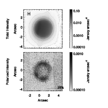
Figure 6.— Uranus, as seen in polarized $H$ band light on 2004 July 05. The upper frame shows total intensity while the lower frame shows polarized intensity with overplotted vectors giving the percent polarization. Uranus is very limb-brightened in polarized light, with a peak polarization of about 1.5% at the edge of its disk. Unlike circumstellar disks, the polarization vectors here point radially inwards rather than circumferentially, an expected effect of Rayleigh scattering in planetary atmospheres. The northern hemisphere, at right, is tilted away from us and noticably less polarized than the nearer southern hemisphere. To our knowledge, this is the first resolved imaging polarimetry of Uranus in the near-infrared, and only the second imaging polarimetry of the planet at any wavelength, after Schmid et al. (2006).

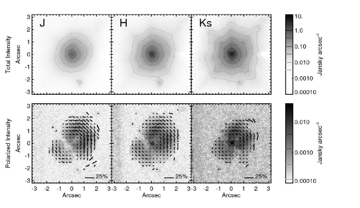
Figure 7.— Multiwavelength imaging polarimetry of the pre-planetary nebula Hen 3-1475. This data shows the power of polarimetry to reveal faint circumstellar material even in the presence of complicated and variable AO PSFs. In total intensity (top row) the circumstellar nebula is not easily visible, but in polarized intensity (bottom row) the symmetric bipolar nebula is clearly detected in all three wavelengths. The morphology seen here compares well with recent HST NICMOS observations presented by Ueta et al. (2007).

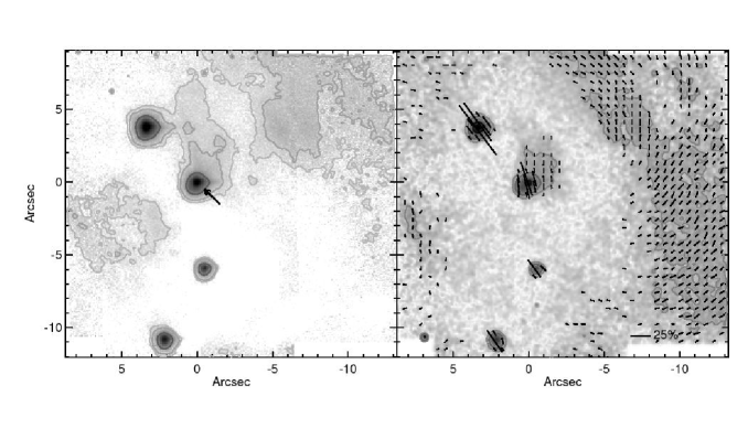
Figure 8.— Laser guide star AO imaging polarimetry of the inner portion of the Crab Nebula, M1, in $H$ band. AO polarimetry can be applied to observe sources of polarization besides dust scattering. Here we observe near-IR synchrotron emission from the Crab Nebula. The arrow indicates the Crab’s central pulsar. Several well known wisps and the knot immediately southeast of the pulsar are visible. The observed morphology and polarization angles are generally consistent with the higher angular resolution observations obtained recently with HST ACS by Hester (2007). Measurement of the degree and orientation of polarization can provide insight into the magnetic field geometry and relatavistic outflow properties. The large field of view shown here was obtained by mosaicing together dithered images comprising 5700 s total exposure time, taken on 2005 Nov 21.

8. Conclusions

We have developed a dual-channel imaging polarimetry mode for the Lick Observatory adaptive optics system and its IRCAL science camera. Its unique YLF Wollaston prism enables differential polarimetry throughout the near infrared, enhancing contrast for the detection of faint circumstellar dust. In practice this system can reduce the stellar PSF halo by a factor of 50-100, ultimately limited by instrumental systematics such as registration and flat-fielding errors. These are the same systematics which have limited other AO polarimeters such as at Gemini (Potter, 2003b) and the VLT (Apai et al., 2004), and we report similar achieved performance to those instruments.

After more than five years of operations, the IRCAL polarimeter has observed targets ranging from young stars to planets to planetary nebulae. A few observations serve to show the capabilities of the IRCAL polarimeter in a variety of scientific contexts. Figure 6 presents the first-ever $H$ band imaging polarimetry of Uranus. Figure 7 shows high-contrast, multiwavelength polarimetry of the circumstellar material around a pre-planetary nebula. Lastly, Figure 8 presents polarization measurements for the synchrotron emission from the inner region of the Crab Nebula, demonstrating that the IRCAL polarimeter can also be used for studies of polarizing processes besides dust scattering.

While the IRCAL polarimeter performs well, it suffers from certain instrumental limitations that could have been avoided had polarimetry been considered during the initial design of the camera. All too many polarimeters are born this way, as post-facto retrofits to instruments originally intended as pure imagers (Hough, 2005). This lesson is particularly relevant to current design efforts for “Extreme AO” high contrast imagers: polarimetric performance should be considered in trade studies early in the design process of both AO systems and science cameras. Present AO polarimeters (in every instance retrofitted into existing instruments) have ably demonstrated their ability to detect faint scattered light in the presence of a bright stellar PSF—the potential for discovery using a truly optimized AO polarimeter is tremendous. In IRCAL’s case, one of the major difficulties is accurately registering undersampled or core-saturated images. Future polarimeters should avoid this by having a well-sampled detector and using “satellite PSFs”, essentially intentional ghost images, to allow the precise registration of images with saturated (or coronagraphically occulted) PSF cores.

An even more promising technique would be to split the polarizations only after pixellating the image plane, entirely eliminating the subpixel registration problem and partially mitigating the effects of uncertain flat fields. Several recent designs for high contrast imaging spectrographs use focal plane lenslet arrays to chop the PSF into pixels prior to wavelength dispersion, to reduce non-common-path optical errors (e.g. Marois et al., 2004, 2005). Experiments to validate these designs are currently underway both in the laboratory (Lafrenière et al., 2006) and on the sky with OSIRIS at Keck (Larkin et al., 2006). Recent results are promising, but differential refraction (both atmospheric and in AO system dichroics) poses complications. However, for polarimetric applications, differential refraction is much less of an issue, and the ability to modulate the polarization provides robustness against non-common-path errors. Lenslet-based differential polarimeters deserve careful study as part of the high contrast astronomer’s future toolkit. As an added bonus, such an instrument would be immune to lateral chromatism, eliminating the need for exotic materials such as YLF.

We end with a brief list of lessons learned from IRCAL, applicable to the design of future high contrast polarimeters. Starlight suppression of about 2 orders of magnitude is attainable with IRCAL and all its flaws. A goal of 3 orders of magnitude suppression seems not unrealistic for future instruments.

1. Low repeatability of the aperture and filter wheel mechanisms in IRCAL complicates data taking and reduction, but is not insurmountable. Any reasonable future design will improve on IRCAL in this regard.

2. Repeatability of mechanisms is particularly important as there are stringent requirements on flat fielding, and IRCAL’s mechanism nonrepeatability prevents the development of high signal-to-noise flat libraries.

3. The Wollaston prism should ideally be located after the cold pupil, to prevent pupil shear between the two polarized beams.

4. To minimize instrumental polarization, the waveplate should be located as far upstream as possible. However, optimized scaled subtraction offers an effective way to empirically remove instrumental (and interstellar) polarization for applications where absolute polarimetry is not required.

5. Registration errors are a key component of the error budget, particularly for undersampled data or long exposures saturated on the central star. The use of artifical “satellite PSFs” as astrometric references may help solve this problem.

6. Lenslet arrays hold great promise for future high contrast polarimeters, largely eliminating the image registration problem. Post lenslet array, the requirements on lateral chromatism are tremendously relaxed, potentially greatly easing requirements on the beamsplitter.

7. For detecting very faint polarized signals, centrosymmetry histograms provide a useful detection metric, particularly when coupled with numerical uncertainty maps computed as part of the data reduction process.

Appendix A An updated list of materials for infrared Wollaston prisms

A large number of birefringent optical materials can be used to make astronomical Wollaston prisms. Oliva et al. (1997) provides a useful list of some of the best candidates. Since that paper, updated measurements of the optical properties of many of these materials have become available, while other candidate materials have come to light. Table A lists potential materials for near infrared Wollaston prisms, and provides updated values for the birefringence $\Delta n$ and birefringent dispersion parameter $V_{\Delta n}$, while Figure 9 shows both achievable beam separations and birefringent optical properties for there materials.

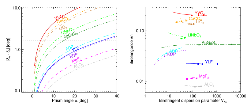
Figure 9.— Left: Beam separation angle as a function of Wollaston prism angle, for birefringent materials from Table A. More birefringent materials are higher in this plot, and require a smaller prism angle to acheive a given beam separation. The horizontal line marks the desired separation for IRCAL. Right: Birefringence versus birefringent dispersion for these materials. This is the birefringent version of the standard Abbe plot for optical materials. On the horizontal axis, the birefringent dispersion parameter $V_{\Delta n}$ measures how much birefringence varies with wavelength, with higher numbers indicating less variation (see §2). Imaging polarimeters benefit from materials whose birefringence is more constant with wavelength (high $V_{\Delta n}$), such as YLF and AgGaS₂. For each material, we show the change in these birefringent parameters from 1-2.5 $\mu m$. Triangles, circles, and squares denote the central wavelengths of $J$, $H$, and $K_{s}$ respectively.

Table 1Materials for Infrared Wollastons

Material	$n$	$\Delta{n}$	$V_{\Delta{n}},J$	$V_{\Delta{n}},H$	$V_{\Delta{n}},K$	References
GaSe	2.74	0.3195	157	135	484	1
Ag3As3	2.77	0.2231	41	72	108	2
YVO4	2.15	0.2053	97	172	278	3
CaCO3	1.63	0.1550	50	33	21	4
Ag3SBs3	2.83	0.1424	37	66	102	2
LiO3	1.85	0.1367	107	109	86	2
BBO	1.64	0.1158	1367	175	87	2
LiNbO3	2.21	0.0728	48	45	33	2
AgGaS2	2.42	0.0535	227	4152	11210	5, 6
BABF	1.61	0.0397	19	14	9	7
ADP	1.48	0.0261	7	-	-	8
YLF	1.44	-0.0220	268	1072	169	9
KDP	1.48	0.0208	5	-	-	10
MgF2	1.37	-0.0113	135	89	56	11
Al2O3	1.74	0.0078	235	213	122	12
KTiOAsO4	1.79	-0.0055	56	26	17	1

Note. — Materials are ordered by decreasing birefringence. The index of refraction, $n$, and birefringence, $\Delta{n}$, are stated for 1.65 $\mathrm{\ \mu{m}}$. The polarization dispersion parameters $V_{\delta{n}}$ were calculated assuming filter bandpasses of 20%, centered on 1.25, 1.65, and 2.1 $\mathrm{\ \mu{m}}$. Dashes indicate wavelength ranges where accurate index of refraction information was not available. More detailed tables of optical properties and software implementing Sellmeier models for all these materials is available from the authors.

References. — 1: Allakhverdiev et al. (2005) 2: Weber (2003) 3: Lomheim & DeShazer (1978) 4: Ghosh (1999) 5: Willer et al. (2001) 6: Takaoka & Kato (1999) 7: Hu et al. (2002) 8: CASIX data sheet, http://www.u-oplaz.com/crystals/crystals07.htm 9: Barnes & Gettemy (1980) 10: Redoptronics data sheet, http://www.optical-components.com/KDP-crystal.html 11: Tropf (1995) 12: Kaplan & Thomas (2003)

References

- Adamson et al. (2005) Adamson, A., Aspin, C., et al., eds. Astronomical Polarimetry: Current Status and Future Directions. 2005
- Ageorges & Walsh (1999) Ageorges, N. & Walsh, J. R. A&AS, 138, 1999, 163
- Aime & Soummer (2004) Aime, C. & Soummer, R. ApJ, 612, 2004, L85
- Allakhverdiev et al. (2005) Allakhverdiev, K., Baykara, T., et al. Journal of Applied Physics, 2005
- Apai et al. (2004) Apai, D., Pascucci, I., et al. A&A, 415, 2004, 671
- Barnes & Gettemy (1980) Barnes, N. & Gettemy, D. Journal of the Optical Society of America, 1980
- Barth (2001) Barth, A. J. In F. R. Harnden, Jr., F. A. Primini, & H. E. Payne, eds., “Astronomical Data Analysis Software and Systems X,” vol. 238 of Astronomical Society of the Pacific Conference Series. 2001, 385–+
- Bauman et al. (2002) Bauman, B. J., Gavel, D. T., et al. In “Proc. SPIE Vol. 4494, p. 19-29, Adaptive Optics Systems and Technology II, Robert K. Tyson; Domenico Bonaccini; Michael C. Roggemann; Eds.”, vol. 4494. 2002, 19–29
- Beuzit et al. (2006) Beuzit, J.-L., Feldt, M., et al. The Messenger, 125, 2006, 29
- Boccaletti et al. (2003) Boccaletti, A., Augereau, J.-C., et al. ApJ, 585, 2003, 494
- Born & Wolf (1959) Born, M. & Wolf, E. Principles of Optics. London: Pergamon Press, 1959, 1959
- Breckinridge & Oppenheimer (2004) Breckinridge, J. B. & Oppenheimer, B. R. ApJ, 600, 2004, 1091
- Chandrasekhar (1946) Chandrasekhar, S. ApJ, 104, 1946, 110
- Clampin et al. (2003) Clampin, M., Krist, J. E., et al. AJ, 126, 2003, 385
- Cronin et al. (2006) Cronin, T., Warrant, E., et al. Applied Optics, 2006
- Fitzgerald & Graham (2006) Fitzgerald, M. P. & Graham, J. R. ApJ, 637, 2006, 541
- Fruchter & Hook (2002) Fruchter, A. S. & Hook, R. N. PASP, 114, 2002, 144
- Gehrels (1974) Gehrels, T., ed. Planets, stars and nebulae studied with photopolarimetry. 1974
- Ghosh (1999) Ghosh, G. Optics Communications, 163, 1999, 95
- Gledhill et al. (1991) Gledhill, T. M., Scarrott, S. M., et al. MNRAS, 252, 1991, 50P
- Graham et al. (2007) Graham, J. R., Kalas, P. G., et al. ApJ, 654, 2007, 595
- Harrington et al. (2006) Harrington, D. M., Kuhn, J. R., et al. PASP, 118, 2006, 845
- Hartkopf et al. (2001) Hartkopf, W. I., Mason, B. D., et al. AJ, 122, 2001, 3472
- Hawarden et al. (2001) Hawarden, T. G., Leggett, S. K., et al. MNRAS, 325, 2001, 563
- Heiles (2000) Heiles, C. AJ, 119, 2000, 923
- Hester (2007) Hester, J. J. In “American Astronomical Society Meeting Abstracts,” vol. 211 of American Astronomical Society Meeting Abstracts. 2007, 100.26
- Hines & Schneider (2006) Hines, D. C. & Schneider, G. In A. M. Koekemoer, P. Goudfrooij, & L. L. Dressel, eds., “The 2005 HST Calibration Workshop: Hubble After the Transition to Two-Gyro Mode,” 2006, 153–+
- Hinkley et al. (2007) Hinkley, S., Oppenheimer, B. R., et al. ApJ, 654, 2007, 633
- Hodapp et al. (2007) Hodapp, K.-W., Tamura, M., et al. In “American Astronomical Society Meeting Abstracts,” vol. 210 of American Astronomical Society Meeting Abstracts. 2007
- Hough (2005) Hough, J. H. In A. Adamson, C. Aspin, & C. Davis, eds., “Astronomical Society of the Pacific Conference Series,” 2005, 3–+
- Hough et al. (2006) Hough, J. H., Lucas, P. W., et al. PASP, 118, 2006, 1305
- Hu et al. (2002) Hu, Z., Yoshimura, M., et al. Jpn. J. Appl. Phys, 2002
- Kaplan & Thomas (2003) Kaplan, S. & Thomas, M. In “Proceedings of SPIE, Vol. 4822,” 2003, 41–50
- Keller (2002) Keller, C. U. In J. Trujillo-Bueno, F. Moreno-Insertis, & F. Sánchez, eds., “Astrophysical Spectropolarimetry,” 2002, 303–354
- Kemp et al. (1987) Kemp, J. C., Henson, G. D., et al. Nature, 326, 1987, 270
- Kuhn et al. (1991) Kuhn, J. R., Lin, H., et al. PASP, 103, 1991, 1097
- Kuhn et al. (2001) Kuhn, J. R., Potter, D., et al. ApJ, 553, 2001, L189
- Lafrenière et al. (2006) Lafrenière, D., Doyon, R., et al. In “Ground-based and Airborne Instrumentation for Astronomy. Edited by Ian S. McLean and Masanori Iye. Proceedings of the SPIE, Volume 6269, pp. 626929 (2006).”, 2006
- Larkin et al. (2006) Larkin, J., Barczys, M., et al. In “Ground-based and Airborne Instrumentation for Astronomy. Edited by Ian S. McLean and Masanori Iye. Proceedings of the SPIE, Volume 6269, pp. 626919 (2006).”, 2006
- Lloyd et al. (2000) Lloyd, J. P., Liu, M. C., et al. In “Proc. SPIE Vol. 4008, p. 814-821, Optical and IR Telescope Instrumentation and Detectors, Masanori Iye; Alan F. Moorwood; Eds.”, vol. 4008. 2000, 814–821
- Lomheim & DeShazer (1978) Lomheim, T. & DeShazer, L. Journal of Applied Physics, 49, 11, 1978, 5517
- Lucas et al. (2004) Lucas, P. W., Fukagawa, M., et al. MNRAS, 352, 2004, 1347
- Macintosh et al. (2006) Macintosh, B., Graham, J., et al. In “Advances in Adaptive Optics II. Edited by Ellerbroek, Brent L.; Bonaccini Calia, Domenico. Proceedings of the SPIE, Volume 6272, pp. (2006).”, 2006
- Marois et al. (2005) Marois, C., Doyon, R., et al. PASP, 117, 2005, 745
- Marois et al. (2006) Marois, C., Lafrenière, D., et al. ApJ, 647, 2006, 612
- Marois et al. (2004) Marois, C., Racine, R., et al. ApJ, 615, 2004, L61
- Masiero et al. (2007) Masiero, J., Hodapp, K., et al. PASP, 119, 2007, 1126
- Max et al. (1997) Max, C., Olivier, S., et al. Science, 277, 1997, 1649
- Oliva (1997) Oliva, E. A&AS, 123, 1997, 589
- Oliva et al. (1997) Oliva, E., Gennari, S., et al. A&AS, 123, 1997, 179
- Patat & Romaniello (2006) Patat, F. & Romaniello, M. PASP, 118, 2006, 146
- Perrin et al. (2006) Perrin, M. D., Duchene, G., et al. ApJ, 645, 2006, 1272
- Perrin et al. (2004a) Perrin, M. D., Graham, J. R., et al. Science, 303, 2004a, 1345
- Perrin et al. (2004b) Perrin, M. D., Graham, J. R., et al. In “Advancements in Adaptive Optics. Edited by Domenico B. Calia, Brent L. Ellerbroek, and Roberto Ragazzoni. Proceedings of the SPIE, Volume 5490, pp. 309-320 (2004).”, 2004b, 309–320
- Persson et al. (1998) Persson, S. E., Murphy, D. C., et al. AJ, 116, 1998, 2475
- Piotto et al. (2002) Piotto, G., King, I. R., et al. A&A, 391, 2002, 945
- Potter & Graham (2005) Potter, D. & Graham, M. Bulletin of the American Astronomical Society, 37, 2005, 1441
- Potter (2003a) Potter, D. E. Ph.D. Thesis, 2003a
- Potter (2003b) Potter, D. E. Ph.D. Thesis, University of Hawaii, 2003b
- Racine et al. (1999) Racine, R. ., Walker, G. A. H., et al. PASP, 111, 1999, 587
- Roberts et al. (2004) Roberts, L. C., Jr., Perrin, M. D., et al. In D. Bonaccini Calia, B. L. Ellerbroek, & R. Ragazzoni, eds., “Advancements in Adaptive Optics. Edited by Domenico B. Calia, Brent L. Ellerbroek, and Roberto Ragazzoni. Proceedings of the SPIE, Volume 5490, pp. 504-515 (2004).”, 2004, 504–515
- Schmid et al. (2006) Schmid, H. M., Joos, F., et al. A&A, 452, 2006, 657
- Sheehy et al. (2006) Sheehy, C. D., McCrady, N., et al. ApJ, 647, 2006, 1517
- Silber et al. (2000) Silber, J., Gledhill, T., et al. ApJ, 536, 2000, L89
- Simmons & Stewart (1985) Simmons, J. F. L. & Stewart, B. G. A&A, 142, 1985, 100
- Sivaramakrishnan & Oppenheimer (2006) Sivaramakrishnan, A. & Oppenheimer, B. R. ApJ, 647, 2006, 620
- Stewart (1991) Stewart, B. G. A&A, 246, 1991, 280
- Stokes (1852) Stokes, G. G. Trans. Camb. Phil. Soc, 9, III, 1852, 399
- Takaoka & Kato (1999) Takaoka, E. & Kato, K. Appl. Opt, 1999
- Tinbergen (1996) Tinbergen, J. Astronomical polarimetry. Cambridge, New York: Cambridge University Press, —c1996, ISBN 0521475317, 1996
- Tropf (1995) Tropf, W. Optical Engineering, 34, 1995, 1369
- Ueta et al. (2007) Ueta, T., Murakawa, K., et al. AJ, 133, 2007, 1345
- Wardle & Kronberg (1974) Wardle, J. F. C. & Kronberg, P. P. ApJ, 194, 1974, 249
- Weber (2003) Weber, M. Handbook of Optical Materials. CRC Press, 2003
- Weinberger et al. (1999) Weinberger, A. J., Becklin, E. E., et al. ApJ, 525, 1999, L53
- Willer et al. (2001) Willer, U., Blanke, T., et al. Applied Optics, 40, 2001, 5439
- Wollaston (1820) Wollaston, W. H. Philosophical Transactions of the Royal Society of London, 110, 1820, 126
- Wolstencroft et al. (1995) Wolstencroft, R. D., Scarrott, S. M., et al. Ap&SS, 224, 1995, 395