Symmetric links and Conway sums:
volume and Jones polynomial

Abstract.

We obtain bounds on hyperbolic volume for periodic links and Conway sums of alternating tangles. For links that are Conway sums we also bound the hyperbolic volume in terms of the coefficients of the Jones polynomial.

1. Introduction

Given a combinatorial diagram of a knot in the 3–sphere, there is an associated 3–manifold, the knot complement, which decomposes into geometric pieces by work of Thurston [26]. A central goal of modern knot theory is to relate this geometric structure to simple topological properties of the knot and to combinatorial knot invariants. To date, there are only a handful of results along these lines. Lackenby found bounds on the volume of alternating links based on the number of twist regions in the link diagram [16]. We extended these results to all links with at least seven crossings per twist region in [12], and in [11] we obtain similar results for links that are closed 3–braids. Our method is to apply a result bounding the change of volume under Dehn filling based on the length of the shortest filling slope. In all these cases the relation between twist number and volume was also important in establishing a coarse volume conjecture: a linear correlation between the coefficients of the classical Jones polynomial and the volume of hyperbolic links.

In the present paper, we build upon the methods of [12] as well as very recent work of Gabai, Meyerhoff, and Milley [13]; Agol, Storm, and Thurston [8]; and Agol [6]. We use this work to give explicit estimates on the volume for links with symmetries of order at least six, and to give estimates on the volume and coefficients of the Jones polynomial under Conway summation of tangles. As in the results above, we obtain explicit linear bounds on volume in terms of the twist number of a diagram.

1.1. Links with high order of symmetry

A link $K$ is called periodic with period an integer $p>1$ if there exists an orientation–preserving diffeomorphism $h\colon\thinspace{S}^{3}\rightarrow{S}^{3}$ of order $p$, such that $h(K)=K$ and either $h$ has fixed points or $h^{i}$ has no fixed points for all $0<i<p$. The solutions to the Smith conjecture [23] and the spherical spaceforms conjecture [22] imply that $h$ is conjugate to an element of $SO(4)$. Thus, if $h$ has no fixed points, the group generated by $h$ acts freely on $S^{3}$ and the quotient of $S^{3}$ is a lens space $L(p,q)$. Furthermore, the quotient of $S^{3}{\smallsetminus}K$ is a link complement in $L(p,q)$. Otherwise, the orthogonal action conjugate to $h$ must be a $2\pi/p$ rotation about a great circle $C_{h}\subset S^{3}$, and the quotient is still $S^{3}$. When the axis $C_{h}$ is either a component of $K$ or disjoint from $K$ (in particular, when $p>2$), the quotient of $K$ is a link $K^{\prime}\subset S^{3}$.

Theorem 1.1.

Let $K$ be a hyperbolic periodic link in $S^{3}$. Assume that the period of $K$ is $p\geq 6$, and acts by rotation about an axis $C_{h}$. Let $K^{\prime}$ be the quotient of $K$. Then

$${\rm vol}(S^{3}{\smallsetminus}K)\;\geq\>p\,\left(1-\frac{2\sqrt{2}\pi^{2}}{p^{2}}\right)^{3/2}{\rm vol}(S^{3}{\smallsetminus}K^{\prime}).$$

In the statement above, $S^{3}{\smallsetminus}K^{\prime}$ may or may not be hyperbolic. We let ${\rm vol}(S^{3}{\smallsetminus}K^{\prime})$ denote simplicial volume, i.e. the sum of the volumes of the hyperbolic pieces in the geometric decomposition of $S^{3}{\smallsetminus}K^{\prime}$.

We combine Theorem 1.1 with a result of Agol, Storm, and Thurston (see Theorem 2.2) to give a bound in terms of the diagram of $K^{\prime}$. We first make the following definitions.

Definition 1.2.

For a knot or link $K$, we consider a diagram $D(K)$ as a 4–valent graph in the plane, with over–under crossing information at each vertex. A link diagram $D$ is called prime if any simple closed curve that meets two edges of the diagram transversely bounds a region of the diagram with no crossings.

Two crossings of a link diagram $D$ are defined to be equivalent if there is a simple closed curve in the plane meeting $D$ in just those crossings. An equivalence class of crossings is defined to be a twist region. The number of distinct equivalence classes is defined to be the twist number of the diagram, and is denoted ${\mathrm{tw}(D)}$.

Our definition of twist number agrees with that in [8], and differs slightly from that in [12]. The two definitions agree provided the diagram is sufficiently reduced (i.e. twist reduced in [12]). We prefer Definition 1.2 as it does not require us to further reduce diagrams.

Corollary 1.3.

With the notation and setting of Theorem 1.1 suppose, moreover, that $K^{\prime}$ is alternating and hyperbolic, with prime alternating diagram $D^{\prime}$. Then

$${{\rm vol}(S^{3}{\smallsetminus}K)}\>\geq\>\left(1-\frac{2\sqrt{2}\pi^{2}}{p^{2}}\right)^{3/2}\,p\,v_{8}\,\left(\frac{{\mathrm{tw}}(D^{\prime})}{2}-1\right),$$

where $v_{8}=3.6638\dots$ is the volume of a regular ideal octahedron in ${\mathbb{H}}^{3}$.

By combining Theorem 1.1 with recent results by Agol [6] and Gabai, Meyerhoff, and Milley [13], we obtain a universal estimate for the volumes of periodic links. For ease of notation, define the function $\psi\colon\thinspace\{x\in{\mathbb{R}}\,\colon\thinspace\,x{\geq 5.5}\}\to{\mathbb{R}}$ by

$$\psi(x):=\min\left\{2.828,\>3.647\left(1-\frac{2\sqrt{2}\,\pi^{2}}{x^{2}}\right)^{3/2}\right\}.$$

Note that the right–hand term in the definition of $\psi$ is greater than $2.828$ for $x\geq 14$.

Theorem 1.4.

Let $K$ be a hyperbolic periodic link in $S^{3}$, of period $p\geq 6$, where we allow freely periodic links as well as those in which the symmetry acts by rotation. Then either

1. ${\rm vol}(S^{3}{\smallsetminus}K)\>\geq\>p\cdot\psi(p)$, or

2. $K$ is one of two explicit exceptions: a $5$–component link of period $10$ whose quotient is $L(10,3){\smallsetminus}{\tt m003}$ or a $5$–component link of period $15$ whose quotient is $L(15,4){\smallsetminus}{\tt m006}$. Here, ${\tt m003}$ and ${\tt m006}$ are manifolds in the SnapPea census; each of these two manifolds is the complement of a unique knot in the respective lens space.

The estimate (1) is sharp for four freely periodic links, whose periods are $14$, $18$, $19$, and $21$.

1.2. Tangles and volumes

A tangle diagram $T$ (or simply a tangle) is a graph contained in a unit square in the plane, with four 1–valent vertices at the corners of the square, and all other vertices 4–valent in the interior. Just as with knot diagrams, every 4–valent vertex of a tangle diagram comes equipped with over–under crossing information. Label the four 1–valent vertices as NW, NE, SE, SW, positioned accordingly.

A tangle diagram is defined to be prime if, for any simple closed curve contained within the unit square which meets the diagram transversely in two edges, the bounded interior of that curve contains no crossings. Two crossings in a tangle are equivalent if there is a simple closed curve in the unit square meeting $D$ in just those crossings. Equivalence classes are called twist regions, and the number of distinct classes is the twist number of the tangle.

An alternating tangle is called positive if the NE strand leads to an over-crossing, and negative if the NE strand leads to an under-crossing.

The closure of a tangle is defined to be the link diagram obtained by connecting NW to NE and SW to SE by crossing–free arcs on the exterior of the disk. A tangle sum, also called a Conway sum, of tangles $T_{1},\dots,T_{n}$ is the closure of the tangle obtained by connecting diagrams of the tangles $T_{1},\dots,T_{n}$ linearly west to east. Notice that if $T_{1},\dots,T_{n}$ are all positive or all negative, their tangle sum will be an alternating diagram.

Finally, we will call a tangle diagram $T$ an east–west twist if ${\mathrm{tw}}(T)=1$ and the diagram consists of a string of crossings running from east to west. The closure of such a diagram gives a standard diagram of a $(2,q)$ torus link.

Theorem 1.5.

Let $T_{1},\dots,T_{n}$, $n\geq 12$, be tangles admitting prime, alternating diagrams, none of which is an east–west twist. Let $K$ be a knot or link which can be written as the Conway sum of the tangles $T_{1},\dots,T_{n}$, with diagram $D$. Then $K$ is hyperbolic, and

$$\frac{v_{8}}{2}\left(1-\left(\frac{8\pi}{11.524+n\sqrt[4]{2}}\right)^{2}\right)^{3/2}\left({\mathrm{tw}}(D)-3\right)\>\leq\>{\rm vol}(S^{3}-K)\><\>10\,v_{3}\,({\mathrm{tw}}(D)-1).$$

Here, $v_{3}=1.0149\dots$ is the volume of a regular ideal tetrahedron and $v_{8}=3.6638\dots$ is the volume of a regular ideal octahedron in ${\mathbb{H}}^{3}$.

The upper bound is due to Agol and D. Thurston [16]. The lower bound approaches $(v_{8}/2)({\mathrm{tw}(D)}-3)$ as the number of tangles $n$ approaches infinity – similar to the (sharp) lower bound for alternating diagrams proved by Agol, Storm, and Thurston [8]. However, Theorem 1.5 applies to more classes of knots than alternating. For example, it applies to large classes of arborescent links (e.g. Montesinos links of length at least 12). In fact, our method of proof applies to links that are obtained by summing up any number of “admissible” tangles, where the term admissible includes, but is not limited to, alternating tangles, tangles that admit diagrams containing at least seven crossings per twist region and tangles whose closures are links of braid index $3$.

1.3. Jones polynomial relations

The volume conjecture of Kashaev and Murakami-Murakami asserts that the volume of hyperbolic knots is determined by certain asymptotics of the Jones polynomial and its relatives. At the same time, recent results [10, 12] combined with a wealth of experimental evidence suggest a coarse version of the volume conjecture: that the coefficients of the Jones polynomial of a hyperbolic link should determine the volume of its complement, up to bounded constants. To state the contribution of the current paper to this coarse volume conjecture we need some notation. For a link $K$, we write its Jones polynomial in the form

$$J_{K}(t)=\alpha t^{k}+\beta t^{k-1}+\ldots+\beta^{\prime}t^{m+1}+\alpha^{\prime}t^{m},$$

so that the second and next-to-last coefficients of $J_{K}(t)$ are $\beta$ and $\beta^{\prime}$, respectively. Dasbach and Lin proved [10] that if $D(K)$ is a prime, alternating diagram, then ${\mathrm{tw}}(D)={\left|\beta\right|}+{\left|\beta^{\prime}\right|}$. In [12], we extended their results to give relations between the coefficients of the Jones polynomial of links and the twist number of link projections that contain at least three crossings per twist region. We further extend the result here.

Above, we defined the closure of a tangle (also called the numerator closure) to be the link diagram obtained by connecting NW to NE and SW to SE by simple arcs with no crossings. The denominator closure of the tangle is defined to be the diagram obtained by connecting NW to SW, and NE to SE by simple arcs with no crossings. We say that a tangle diagram $T$ is strongly alternating if it is alternating and both the numerator and denominator closures define prime diagrams.

Theorem 1.6.

Let $T_{1},\dots,T_{n}$ be alternating tangles whose Conway sum is a knot $K$ with diagram $D$. Define $T_{+}$ to be the result of joining all the positive $T_{i}$ west to east, $T_{-}$ to be the result of joining all the negative $T_{i}$ west to east. Then, if both $T_{+}$ and $T_{-}$ are strongly alternating,

$$\frac{{\mathrm{tw}(D)}}{2}-2\;\leq\;{\left|\beta\right|}+{\left|\beta^{\prime}\right|}\;\leq\;2\,{\mathrm{tw}(D)}.$$

If some $T_{i}$ is an east–west twist, then the denominator closure of $T_{+}$ or $T_{-}$ will contain nugatory crossings, failing to be prime. Thus the hypotheses of Theorem 1.6 imply that no $T_{i}$ is an east–west twist. As a result, combining Theorems 1.5 and 1.6 gives

Corollary 1.7.

Let $K$ be a knot which can be written as the Conway sum of tangles $T_{1},\dots,T_{n}$. Let $T_{+}$ and $T_{-}$ be the sums of the positive and negative $T_{i}$, respectively. Suppose that $n\geq 12$, and both $T_{+}$ and $T_{-}$ are strongly alternating. Then $K$ is hyperbolic, and

$$\frac{v_{8}}{4}\,\left(1-\left(\frac{8\pi}{11.524+n\sqrt[4]{2}}\right)^{2}\right)^{3/2}\left({\left|\beta\right|}+{\left|\beta^{\prime}\right|}-6\right)\>\leq\>{\rm vol}(S^{3}-K)\><\>20v_{3}\,\left({\left|\beta\right|}+{\left|\beta^{\prime}\right|}+\frac{3}{2}\right).$$

The hypothesis that $K$ be a knot is crucial in the statements of Theorem 1.6 and Corollary 1.7. Both statements fail, for example, for the family of $(2,\cdots,2,-2,\cdots,-2)$ pretzel links. Theorem 1.5 implies the volume of $K$ will grow in an approximately linear fashion with the number of positive and negative $2$’s. On the other hand, using Lemma 5.1 below one can easily compute that ${\left|\beta\right|}+{\left|\beta^{\prime}\right|}=2$ for this family of links.

1.4. Organization

The proofs of our theorems bring together several very recent results of Agol [6]; Agol, Storm, and Thurston [8]; Gabai, Meyerhoff, and Milley [13]; and the authors [12]. We survey the results in Section 2. In Section 3, we move on to periodic links to prove Theorems 1.1 and 1.4 and establish some corollaries. Then, in Section 4 we use Adams’ “belted sum” operations to study the behavior of hyperbolic volume under the Conway summation of tangles, proving Theorem 1.5. In Section 5 we prove Theorem 1.6.

2. Recent estimates of hyperbolic volume and cusp area

In this section, we survey several recent results by Agol [6], Agol–Storm–Thurston [8], the authors [12], and Gabai–Meyerhoff–Milley [13], which we will apply in later sections. Taken together, these theorems give powerful structural results about the volumes of hyperbolic manifolds. We also prove Theorem 2.7, which follows quickly from the above recent results, and will be important in Section 4.

2.1. Estimates from guts

Let $M$ be a hyperbolic $3$–manifold, and $S\subset M$ an essential surface. When we cut $M{\smallsetminus}S$ along essential annuli, it decomposes into a characteristic submanifold $B$ (the union of all $I$–bundles in $M{\smallsetminus}S$), and a hyperbolic component called ${\rm guts}(M,S)$. Using Perelman’s estimates for volume change under Ricci flow with surgery, Agol, Storm, and Thurston proved the following result.

Theorem 2.1 (Theorem 9.1 of [8]).

Let $M$ be a finite–volume hyperbolic $3$–manifold, and let $S\subset M$ be an essential surface. Then

$${\rm vol}(M)\geq-v_{8}\,\chi({\rm guts}(M,S)).$$

Combining Theorem 2.1 with Lackenby’s analysis of checkerboard surfaces in alternating link complements [16] gives the following result, which bounds volume based on diagrammatic properties.

Theorem 2.2 (Corollary 2.2 of [8]).

Let $D(K)$ be a prime, alternating link diagram with ${\mathrm{tw}(D)}\geq 2$. Then $K$ is hyperbolic, and

$${\rm vol}(S^{3}{\smallsetminus}K)\geq\frac{v_{8}}{2}\,({\mathrm{tw}(D)}-2).$$

More recently, Agol showed that every two–cusped hyperbolic $3$–manifold contains an essential surface with non-trivial guts [6]. Using Theorem 2.1, he obtained

Theorem 2.3 (Theorem 3.4 of [6]).

Let $M$ be an orientable hyperbolic $3$–manifold with two or more cusps. Then

$${\rm vol}(M)\geq v_{8},$$

with equality if and only if $M$ is the complement of the Whitehead link or its sister (m129 or m125 in the notation of the SnapPea census).

2.2. Bounding volume change under Dehn filling

Given a 3–manifold $M$ with at least $k$ torus boundary components, we use the following standard terminology. For the $i$-th torus $T_{i}$, let $s_{i}$ be a slope on $T_{i}$, that is, an isotopy class of simple closed curves. Let $M(s_{1},\dots,s_{k})$ denote the manifold obtained by Dehn filling along the slopes $s_{1}$, …, $s_{k}$.

When $M$ is hyperbolic, each torus boundary component of $M$ corresponds to a cusp. Taking a maximal disjoint horoball neighborhood about each of the cusps, each torus $T_{i}$ inherits a Euclidean structure, well–defined up to similarity. The slope $s_{i}$ can then be given a geodesic representative. We define the slope length of $s_{i}$ to be the length of this geodesic representative. Note that when $k>1$, this definition of slope length depends on the choice of maximal horoball neighborhood. The authors recently showed the following result.

Theorem 2.4 (Theorem 1.1 of [12]).

Let $M$ be a complete, finite–volume hyperbolic manifold with cusps. Suppose $C_{1},\dots,C_{k}$ are disjoint horoball neighborhoods of some subset of the cusps. Let $s_{1},\dots,s_{k}$ be slopes on $\partial C_{1},\dots,\partial C_{k}$, each with length greater than $2\pi$. Denote the minimal slope length by ${\ell_{\rm min}}$. Then $M(s_{1},\dots,s_{k})$ is a hyperbolic manifold, and

$${\rm vol}(M(s_{1},\dots,s_{k}))\>\geq\>\left(1-\left(\frac{2\pi}{{\ell_{\rm min}}}\right)^{2}\right)^{3/2}{\rm vol}(M).$$

2.3. Mom technology

In a series of recent papers [14, 13, 21], Gabai, Meyerhoff, and Milley developed the theory of Mom manifolds. A Mom-n structure $(M,T,\Delta)$ consists of a compact 3–manifold $M$ whose boundary is a union of tori, a preferred boundary component $T$, and a handle decomposition $\Delta$ of the following type. Starting from $T\times I$, $n$ 1–handles and $n$ 2–handles are attached to $T\times 1$ such that each 2–handle goes over exactly three 1–handles, counted with multiplicity. Furthermore, each 1–handle encounters at least two 2–handles, counted with multiplicity. We say that $M$ is a Mom-n if it possesses a Mom-$n$ structure $(M,T,\Delta)$.

In [14], Gabai, Meyerhoff, and Milley enumerated all the hyperbolic Mom-2’s and Mom-3’s (there are 21 such manifolds in total). In [13], they showed that every cusped hyperbolic manifold of sufficiently small volume (or cusp area) must be obtained by Dehn filling a Mom-2 or Mom-3 manifold:

Theorem 2.5 ([13]).

Let $M$ be a cusped, orientable hyperbolic $3$–manifold. Assume that ${\rm vol}(M)\leq 2.848$ or that a maximal horoball neighborhood $C$ of one of its cusps has ${\rm area}({\partial}C)\leq 3.78$. Then $M$ is obtained by Dehn filling on one of the 21 Mom-2 or Mom-3 manifolds.

Proof.

The volume part of the theorem is explicitly stated as Theorem 1.1 of [13]. The cusp area part of the statement follows by evaluating Gabai, Meyerhoff, and Milley’s cusp area estimates [13, Lemmas 4.6, 4.8, 5.4, 5.6, and 5.7] on the parameter space of all ortholengths corresponding to manifolds without a Mom-2 or Mom-3 structure. The rigorous C++ and Mathematica code to construct and evaluate those estimates was helpfully supplied by Milley [20]. ∎

Because each of the Mom-2 and Mom-3 manifolds has volume significantly higher than 2.848, Theorem 2.4 bounds the length of the slope along which one must fill a Mom manifold to obtain $M$. Thus, Theorem 2.5 combined with Theorem 2.4 reduces the search for small–volume manifolds to finitely many Dehn fillings of the 21 Mom-2’s and Mom-3’s.

Corollary 2.6 (Theorem 1.2 of [21]).

Let $M$ be a cusped, orientable hyperbolic manifold whose volume is at most $2.848$. Then $M$ is one of the SnapPea census manifolds m003, m004, m006, m007, m009, m010, m011, m015, m016, or m017. In particular, every cusped hyperbolic manifold with ${\rm vol}(M)\leq 2.848$ can be obtained by Dehn filling two cusps of the $3$–chain link complement in Figure 1.

Theorem 2.5 can also be employed to give universal estimates for the cusp area of those manifolds that have two or more cusps:

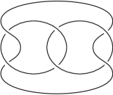
Figure 1. The complement of the $3$–chain link is the only Mom-2 or Mom-3 manifold with more than two cusps.

Theorem 2.7.

Let $M$ be an orientable hyperbolic $3$–manifold with two or more cusps. Suppose that $M$ contains a belt (an essential twice–punctured disk). If $C$ is a maximal neighborhood of one of the cusps of $M$, then

$$\mathrm{area}({\partial}C)\geq 3.78.$$

Remark.

The hypothesis that $M$ contains a belt should be unnecessary. However, proving the theorem without this hypothesis would require studying infinitely many fillings of the $3$–chain link in Figure 1.

Proof.

Theorem 2.5 implies that every cusped hyperbolic manifold either has cusp area at least $3.78$, or is obtained by Dehn filling on one of the Mom-2 or Mom-3 manifolds. Among these 21 Mom manifolds, 20 have exactly two cusps. Thus, if $M$ is obtained by filling on one of these 20 manifolds, the filling must be trivial and it already is one of the Mom manifolds. Individual verification shows that a maximal neighborhood of any cusp of any of the Mom-2 or Mom-3 manifolds has area at least $4$ (with the minimum of $4$ realized by the Whitehead link). Therefore, $M$ either has cusp area at least $3.78$, or is obtained by Dehn filling one cusp of the single $3$–cusped Mom manifold $N$, namely the complement of the $3$–chain link depicted in Figure 1.

Proposition 2.8.

Let $M$ be a hyperbolic $3$–manifold obtained by filling one cusp of the $3$–chain link complement $N$. Suppose that $M$ contains an essential twice–punctured disk. If $C$ is a maximal neighborhood of one of the cusps of $M$, then $\mathrm{area}({\partial}C)\geq 4$.

Proof.

Suppose that $M$ contains an essential twice–punctured disk $P$. Isotope $P$ to minimize its intersection number with the core of the solid torus added during Dehn filling. Then $S=P\cap N$ is an essential surface in $N$; more precisely, it is an essential sphere with $(n+3)$ holes, where $n$ of its boundary circles run in parallel along the filling slope. Since every thrice–punctured sphere in $N$ meets all three cusps (and thus becomes an essential annulus after filling along one of its boundary circles), we can conclude that $n\geq 1$.

Now, expand a maximal horospherical neighborhood $H$ of the cusp of $N$ that we are filling. Consider the length $\ell$ of the filling slope along ${\partial}H$. Since $S\cap{\partial}H$ consists of $n$ distinct circles of that slope, a result of Agol and Lackenby (see [7, Theorem 5.1] or [15, Lemma 3.3]) implies that the total length of those circles is

$$n\,\ell\>\leq\>-6\,\chi(S)\>=\>6(n+1)\>\leq\>12n.$$

Therefore, $M$ is obtained by filling one cusp of $N$ along a slope of length at most $12$.

To complete the proof, we enumerate the slopes that have length at most $12$. Note that since the symmetry group of $N$ permutes all three cusps, it suffices to consider a single cusp. In complex coordinates on this maximal cusp, the knot–theoretic longitude is a translation by $4$, while the meridian is a translation by $\frac{3}{2}+\frac{\sqrt{7}}{2}i$. Thus the slopes on a cusp of $N$ that have length at most $12$ are:

(1) $$\begin{array}[]{c}1/0\\ -7\quad-\!6\quad\cdots\quad 3\quad\>4\\ -7/2\quad-\!5/2\quad-\!3/2\quad-\!1/2\quad\>1/2\\ -8/3\quad-\!7/3\quad-\!5/3\quad-\!4/3\quad-\!2/3\quad-\!1/3\\ -7/4\quad-\!5/4\end{array}$$

Martelli and Petronio [19] have shown that the non-hyperbolic fillings of one cusp of $N$ are exactly the fillings along slope $\infty,-3,-2,-1,\,0$. For each of the $21$ remaining slopes, SnapPea finds (an approximate solution for) a hyperbolic structure on the filled manifold. H. Moser’s thesis [24] then implies that the true hyperbolic structure on each of these manifolds is indeed $\varepsilon$–close to the one found by SnapPea. In each case, the cusp area is bounded below by $4$.∎

Proposition 2.8 completes the proof of Theorem 2.7.∎

As a closing remark, we point out that among the hyperbolic fillings of the $3$–chain link listed in (1), only the Whitehead link complement contains a belt. In other words, a topological analysis of these manifolds shows that the Whitehead link is the only manifold satisfying the hypotheses of Proposition 2.8. Since we do not need this stronger statement in the sequel, we omit the details.

3. Volume estimates for periodic links

Let $K$ be a periodic link and let $h:{S}^{3}\rightarrow{S}^{3}$ be an orientation preserving diffeomorphism of order $p$ with $h(K)=K$, such that the set of fixed points $C_{h}$ of $h$ is a circle that is either disjoint from $K$ or is a component of $K$. By Smith theory and the solution to the Smith conjecture [23], $C_{h}$ is the trivial knot and $h$ is conjugate to a rotation with axis $C_{h}$. The quotient of the action of $h$ on $K$ is a link $K^{\prime}$, called the quotient of $K$. Let $C^{\prime}_{h}$ denote the quotient of the axis $C_{h}$ under the action of $h$ on $S^{3}$.

Theorem 3.1.

Let $K$ be a periodic hyperbolic link in $S^{3}$ of period $p\geq 6$. Let $C^{\prime}_{h}$ be the quotient of the fixed point set under $h$ and let $K^{\prime}$ be the quotient link of $K$. Then, $L_{h}:=K^{\prime}\cup C^{\prime}_{h}$ is a hyperbolic link, and

$$p\;\left(1-\frac{2\sqrt{2}\pi^{2}}{p^{2}}\right)^{3/2}{\rm vol}(S^{3}{\smallsetminus}L_{h})\>\leq\>{\rm vol}(S^{3}{\smallsetminus}K)\>\leq\>p\;{\rm vol}(S^{3}{\smallsetminus}L_{h}).$$

Proof.

The Mostow–Prasad rigidity theorem implies that $h$ can be homotoped to a hyperbolic isometry $h\colon\thinspace S^{3}{\smallsetminus}K\rightarrow S^{3}{\smallsetminus}K$. Since $S^{3}{\smallsetminus}K$ is a Haken 3–manifold, a result of Waldhausen [27] implies that $h$ can actually be isotoped to a hyperbolic isometry. Thus $C_{h}$ is either a component of $K$, or else it is a closed geodesic in $S^{3}{\smallsetminus}K$. It follows that $S^{3}{\smallsetminus}(K\cup C_{h})$ is hyperbolic (in the case that $C_{h}$ is a component of $K$ we take $K\cup C_{h}=K$). Now the quotient of the action $h\colon\thinspace S^{3}{\smallsetminus}(K\cup C_{h})\rightarrow S^{3}{\smallsetminus}(K\cup C_{h})$, which is $S^{3}{\smallsetminus}L_{h}$, is also hyperbolic. The quotient map

$$S^{3}{\smallsetminus}(K\cup C_{h})\longrightarrow S^{3}{\smallsetminus}L_{h}$$

is a covering of degree $p$. Thus

$${\rm vol}(S^{3}{\smallsetminus}(K\cup C_{h}))=p\,{\rm vol}(S^{3}{\smallsetminus}L_{h}).$$

If $C_{h}$ is a component of $K$, we are done. Otherwise, $S^{3}{\smallsetminus}K$ is obtained from $S^{3}{\smallsetminus}(K\cup C_{h})$ by Dehn filling $C_{h}$ along the meridian $m$. This meridian covers the meridian $m^{\prime}$ of $C^{\prime}_{h}$ $p$ times. By work of Adams [1], the length of $m^{\prime}$ satisfies $l(m^{\prime})\geq\sqrt[4]{2}$. Thus, $l(m)\geq p\,\sqrt[4]{2}$. For $p\geq 6$ we have $l(m)\geq p\,\sqrt[4]{2}>2\pi$. Now Theorem 2.4 applies, and we conclude

$${\rm vol}(S^{3}{\smallsetminus}K) \geq \left(1-\frac{2\sqrt{2}\pi^{2}}{p^{2}}\right)^{3/2}{\rm vol}(S^{3}{\smallsetminus}(C_{h}\cup K))$$

$$= \left(1-\frac{2\sqrt{2}\pi^{2}}{p^{2}}\right)^{3/2}\,p\,{\rm vol}(S^{3}{\smallsetminus}L_{h}).$$

As for the upper bound, we note that volume strictly decreases under Dehn filling [25, Corollary 6.5.2]. Thus, if $C_{h}$ is not already a component of $K$, we have

$$p\;{\rm vol}(S^{3}{\smallsetminus}L_{h})={\rm vol}(S^{3}{\smallsetminus}(K\cup C_{h}))>{\rm vol}(S^{3}{\smallsetminus}K).$$

∎

Next we derive Theorem 1.1 from Theorem 3.1: To that end, for a $3$–manifold $M$ we will let $\left\|M\right\|$ denote the Gromov norm of $M$. By [25, Theorem 6.5.4], if $M$ is hyperbolic then ${\rm vol}(M)=v_{3}\left\|M\right\|$. More generally, $v_{3}\left\|M\right\|$ is the simplicial volume of $M$, equal to the sum of volumes of the hyperbolic pieces in the geometric decomposition of $M$.

Proof of Theorem 1.1.

If the axis $C_{h}$ is not already a component of $K$, the complement $S^{3}{\smallsetminus}K^{\prime}$ is obtained by Dehn filling from $S^{3}{\smallsetminus}L_{h}$. We note that $K^{\prime}$ need not be hyperbolic. By [25, Corollary 6.5.2], we have $\left\|S^{3}{\smallsetminus}L_{h}\right\|>\left\|S^{3}{\smallsetminus}K^{\prime}\right\|$. Since, by Theorem 3.1, $L_{h}$ is hyperbolic, ${\rm vol}(S^{3}{\smallsetminus}L_{h})=v_{3}\left\|S^{3}{\smallsetminus}L_{h}\right\|$. Combining these facts with the left-hand inequality of Theorem 3.1 gives

$${\rm vol}(S^{3}{\smallsetminus}K)\geq\left(1-\frac{2\sqrt{2}\pi^{2}}{p^{2}}\right)^{3/2}\,p\,v_{3}\,\left\|S^{3}{\smallsetminus}K^{\prime}\right\|.$$

∎

Now, we turn our attention to Theorem 1.4. Define $\psi\colon\thinspace\{x\in{\mathbb{R}}\,\colon\thinspace\,x{\geq 5.5}\}\to{\mathbb{R}}$ by

$$\psi(x):=\min\left\{2.828,\>3.647\left(1-\frac{2\sqrt{2}\,\pi^{2}}{x^{2}}\right)^{3/2}\right\}.$$

Theorem 3.2 (Theorem 1.4).

Let $K$ be a hyperbolic periodic link in $S^{3}$, of period $p\geq 6$. Then either

1. ${\rm vol}(S^{3}{\smallsetminus}K)\>\geq\>p\cdot\psi(p)$, or

2. $K$ is one of two explicit exceptions: a $5$–component link of period $10$ whose quotient is $L(10,3){\smallsetminus}{\tt m003}$ or a $5$–component link of period $15$ whose quotient is $L(15,4){\smallsetminus}{\tt m006}$.

Estimate (1) is sharp for four freely periodic links, whose periods are $14$, $18$, $19$, and $21$.

Proof.

Let $h:S^{3}\to S^{3}$ be the diffeomorphism of order $p$ that sends $K$ to itself. As discussed in the introduction, the solutions to the Smith conjecture [23] and the spherical spaceforms conjecture [22] imply that we may take $h$ to be an orthogonal action by an element of $SO(4)$. We need to consider two cases: either $h$ fixes an invariant axis $C_{h}$, or $h^{i}$ acts on $S^{3}$ without fixed points, for all $0<i<p$.

If $h$ has an invariant axis $C_{h}$, then Theorem 3.1 applies, and

$${\rm vol}(S^{3}{\smallsetminus}K)\>\geq\>p\;\left(1-\frac{2\sqrt{2}\pi^{2}}{p^{2}}\right)^{3/2}{\rm vol}(S^{3}{\smallsetminus}L_{h}).$$

Now, because $L_{h}$ is a hyperbolic link of two or more components, Agol’s Theorem 2.3 gives ${\rm vol}(S^{3}{\smallsetminus}L_{h})\geq 3.663$, completing the argument in this case.

If $h^{i}$ acts on $S^{3}$ without fixed points, for all $0<i<p$, the quotient of $S^{3}$ is a lens space $L(p,q)$ and the quotient of $S^{3}{\smallsetminus}K$ is a hyperbolic manifold $M$, obtained as the complement of a link in $L(p,q)$. Thus

$${\rm vol}(S^{3}{\smallsetminus}K)=p\cdot{\rm vol}(M).$$

If ${\rm vol}(M)\geq 2.828$, then $K$ satisfies the statement of the theorem. On the other hand, if ${\rm vol}(M)\leq 2.848$, then $M$ is one of the ten one–cusped manifolds listed in Corollary 2.6. Thus, to complete the proof, it suffices to enumerate all of the ways in which each of these ten manifolds occurs as the complement of a knot in a lens space. Because each manifold in Corollary 2.6 is a filling of two cusps of the complement $N$ of the $3$–chain link of Figure 1, we can use the extensive tables compiled by Martelli and Petronio [19, Section A.1] to enumerate their lens space fillings:

Manifold	Alternate name	Volume	Surgery on $N$	Lens space fillings
m003	figure–8 sister	2.0298…	$N(1,-4)$	$L(5,1),\,L(10,3)$
m004	figure–8 knot	2.0298…	$N(1,2)$	$S^{3}$
m006		2.5689…	$N(1,-3/2)$	$L(5,2),\,L(15,4)$
m007		2.5689…	$N(1,-1/2)$	$L(3,1)$
m009	p. torus bundle $LLR$	2.6667…	$N(1,3)$	$L(2,1)$
m010	p. torus bundle $-LLR$	2.6667…	$N(1,-5)$	$L(6,1)$
m011		2.7818…	$N(-3/2,-5)$	$L(9,2),\,L(13,4)$
m015	$5_{2}$ knot	2.8281…	$N(1,1/2)$	$S^{3}$
m016	$(-2,3,7)$ pretzel knot	2.8281…	$N(-3/2,-1/2)$	$S^{3},\,L(18,5),\,L(19,7)$
m017		2.8281…	$N(1,-5/2)$	$L(7,2),\,L(14,3),\,L(21,8)$

The proof will be complete after several observations. First, we may ignore lens spaces $L(p,q)$ with $p\leq 5$, because we have assumed $p\geq 6$. Second, the two exceptions to the theorem are obtained by lifting to $S^{3}$ the knots $(L(10,3){\smallsetminus}{\tt m003})$ and $(L(15,4){\smallsetminus}{\tt m006})$. Homology considerations show that both of these exceptions are $5$–component links. Third, even though $L(6,1)$, $L(9,2)$, and $L(13,4)$ are obtained by filling manifolds of volume less than $2.828$, the corresponding links satisfy the theorem because $3.647\left(1-2\sqrt{2}\,\pi^{2}/6^{2}\right)^{3/2}<2.666$ and

$$3.647\left(1-\frac{2\sqrt{2}\,\pi^{2}}{9^{2}}\right)^{3/2}\><\>\>3.647\left(1-\frac{2\sqrt{2}\,\pi^{2}}{13^{2}}\right)^{3/2}\><\>\>2.7818.$$

Finally, the four examples demonstrating the sharpness of the theorem are the 18–fold and 19–fold covers of ${\tt m016}$ and the 14–fold and 21–fold covers of ${\tt m017}$. ∎

Note that if the link $K$ in Theorem 1.4 is not freely periodic, then the volume is actually bounded by the quantity on the right in the definition of $\psi(n)$.

4. Belted sums and Conway sums

4.1. Belted sums

Let $T$ be a tangle diagram. Given $T$, we may form a link diagram as follows. First, form the closure of $T$ by connecting NE to NW, and SE to SW. Then, add an extra component $C$ that lies in a plane orthogonal to the projection plane and encircles the two unknotted arcs that we have just added to $T$. See the left of Figure 2. We call the resulting link the belted tangle corresponding to $T$, or simply a belted tangle. Note that $C$ bounds a 2–punctured disk $S$ in the complement of the link. We will call the link component $C$ the belt component of the link. We will only be interested in belted tangles admitting hyperbolic structures.

Figure 2. Belted sum.

Given two hyperbolic belted tangles corresponding to $T_{1}$ and $T_{2}$, with complements $M_{1}$ and $M_{2}$, belt components $C_{1}$ and $C_{2}$, and 2–punctured disks $S_{1}$ and $S_{2}$, we form the complement of a new belted tangle as follows. Cut each manifold $M_{i}$ along the surface $S_{i}$, and then glue two manifolds with two 2–punctured disks as boundary. Since there is a unique hyperbolic structure on a 2–punctured disk we may glue $M_{1}$ to $M_{2}$ by an isometry that glues $C_{1}$ to $C_{2}$. The result is the complement of a new belted tangle. See Figure 2. We call this new belted tangle the belted sum of the tangles $T_{1}$ and $T_{2}$. Belted sums were studied extensively by Adams [2]. Note that the Conway sum of $T_{1}$ and $T_{2}$ is obtained by meridional Dehn filling on the belt component of the belted sum of $T_{1}$ and $T_{2}$.

4.2. Arc lengths on belted tangles

Consider a maximal neighborhood $C$ of the cusp corresponding to the belt component. Denote by the width the length of the shortest nontrivial geodesic arc running from the 2–punctured disk to itself on $\partial C$. Adams et al observed that the length of the shortest nontrivial arc from an embedded totally geodesic surface to itself is bounded below by $1$ (see [5, Theorem 4.2] or [4, Theorem 1.5]). In the case at hand, their result gives the following.

Lemma 4.1.

The width of a belt component of a belted tangle is at least $1$.

Note that since the 2–punctured disk intersects the cusp in a longitude, the meridian must be at least as long as the width. We will also need bounds on the length of a longitude.

Lemma 4.2.

The length of the longitude of a belt component is at most $4$, and at least $\sqrt[4]{2}$.

Proof.

Both bounds are due to Adams. In [1], he proves that if $M$ is not the complement of the figure–8 knot or the $5_{2}$ knot, then the shortest curve has length at least $\sqrt[4]{2}$.

As for the upper bound, the length of the longitude is maximal when the maximal cusp in $M$ restricts to a maximal cusp on the 3–punctured sphere. By [3, Theorem 2.1], the length of a maximal cusp on the 3–punctured sphere is $4$. ∎

We need to determine a maximal cusp corresponding to the belt component of a belted sum of two tangles, $T_{1}$ and $T_{2}$. When we expand a horoball neighborhood about this cusp, the cusp neighborhood may bump itself in one component of the belt sum before it bumps in the other. When the cusp bumps itself, it determines a longitude of the belt component. Thus the longitude of the belt component of the belted sum will have length equal to the minimum of the longitude lengths of $T_{1}$ and $T_{2}$. Say this minimum occurs in $T_{1}$. Then the length of any arc running from 3–punctured sphere to 3–punctured sphere in $T_{2}$ will be scaled by the ratio of the length of the longitude of $T_{1}$ and the length of the longitude of $T_{2}$. In particular, the width of the belted sum will not necessarily be the width of $T_{1}$ plus the width of $T_{2}$, but rather the width of $T_{1}$ plus the width of $T_{2}$ times the ratio of the longitude length of $T_{1}$ to the longitude length of $T_{2}$.

Lemma 4.3.

Let $T$ be a belted tangle obtained as the belted sum of $n$ hyperbolic belted tangles $T_{1},\dots,T_{n}$. Let $\ell$ be the length of the shortest longitude of a belt component of the $T_{j}$. Then the width of the belt component of $T$ is at least

$$w\geq\frac{3.78}{\ell}+(n-1)\,\frac{\ell}{4}.$$

Proof.

Without loss of generality, suppose $T_{1}$ has the shortest longitude. By Theorem 2.7, the cusp area corresponding to the belt component is at least $3.78$. Thus the width of $T_{1}$ is at least $3.78/\ell$. By Lemma 4.2, the longitudes of the other $T_{j}$’s are at most $4$, and by Lemma 4.1, the widths of these are at least $1$. When we do the belted sum, the longitudes will rescale to be length $\ell$, and the widths will rescale to be at least $\ell/4$. Thus the total width will be at least $w\geq 3.78/\ell+(n-1)(\ell/4).$ ∎

4.3. Volumes and belted tangles

Lemma 4.4.

Let $T$ be a prime, alternating tangle that is not an east–west twist. Let $L$ denote the belted tangle corresponding to $T$. Then $L$ is hyperbolic. Furthermore,

(A) If $1/n$ Dehn filling along the belt component adds a new twist region to the closure of $T$, then

$${\rm vol}(S^{3}{\smallsetminus}L)\geq\frac{v_{8}}{2}\,({\mathrm{tw}}(T)-1).$$

(B) If $1/n$ Dehn filling along the belt component adds crossings to an existing twist region in the closure of $T$, then

$${\rm vol}(S^{3}{\smallsetminus}L)\geq\frac{v_{8}}{2}\,({\mathrm{tw}}(T)-2).$$

Proof.

Let $L(n)$ denote the link formed by performing $1/n$ Dehn filling on the belt component of $L$, where $n$ is positive or negative depending on which sign makes $L(n)$ alternating. When we form $L(n)$, we may either add a new twist region to the closure of $T$, or we may add additional crossings to an existing twist region. In either case the link $L(n)$ has at least two twist regions, since $T$ is not an east–west twist, hence it is hyperbolic.

In case (A), Theorem 2.2 implies the volume of $S^{3}{\smallsetminus}L(n)$ is at least $v_{8}/2(({\mathrm{tw}}(T)+1)-2)$. In case (B), Theorem 2.2 implies the volume of $S^{3}{\smallsetminus}L(n)$ is at least $v_{8}/2({\mathrm{tw}}(T)-2)$. Because volume goes down under Dehn filling, these lower bounds on the volume of ${\rm vol}(S^{3}{\smallsetminus}L(n))$ also serve as lower bounds on ${\rm vol}(S^{3}{\smallsetminus}L)$. ∎

Lemma 4.5.

Let $T_{1},\ldots,T_{n}$ prime, alternating tangle diagrams, none of which is an east–west twist. Let $D(K)$ be the Conway sum of $T_{1},\ldots,T_{n}$, and let $L$ be the belted sum of these tangles. Then

$${\rm vol}(S^{3}{\smallsetminus}L)\geq\frac{v_{8}}{2}\,({\mathrm{tw}}(D)-3).$$

Proof.

Because we formed the belted sum $L$ by gluing belted tangles along totally geodesic $2$–punctured disks, the volume of $L$ will remain unchanged if we permute the order of the $T_{i}$. Thus, without loss of generality, we may assume that $T_{1},\ldots,T_{r}$ are positive tangles and $T_{r+1},\ldots,T_{n}$ are negative tangles. Furthermore, if the $T_{i}$ are all positive or all negative, then $D(K)$ is a prime, alternating diagram, and the result follows by Lemma 4.4. Thus we may assume that $0<r<n$.

With these assumptions, let $D_{+}$ be the Conway sum and $L_{+}$ be the belted sum of $T_{1},\ldots,T_{r}$. Let $D_{-}$ be the Conway sum and $L_{-}$ be the belted sum of $T_{r+1},\ldots T_{n}$. Then each of $D_{+}$ and $D_{-}$ is the closure of a prime, alternating tangle. Thus, by Lemma 4.4,

$${\rm vol}(S^{3}{\smallsetminus}L_{+})\geq\frac{v_{8}}{2}\,({\mathrm{tw}}(D_{+})-2)\qquad\mbox{and}\qquad{\rm vol}(S^{3}{\smallsetminus}L_{-})\geq\frac{v_{8}}{2}\,({\mathrm{tw}}(D_{-})-2),$$

with a sharper estimate if either $D_{+}$ or $D_{-}$ falls into case (A) of the Lemma.

Suppose that either $D_{+}$ or $D_{-}$ falls into case (A) of Lemma 4.4. Then, since equivalent crossings remain equivalent after gluing, we have ${\mathrm{tw}}(D_{+})+{\mathrm{tw}}(D_{-})\geq{\mathrm{tw}(D)}$, and thus

$${\rm vol}(S^{3}{\smallsetminus}L)\>=\>{\rm vol}(S^{3}{\smallsetminus}L_{+})+{\rm vol}(S^{3}{\smallsetminus}L_{-})\>\geq\>\frac{v_{8}}{2}\,({\mathrm{tw}}(D)-3).$$

On the other hand, suppose that both $D_{+}$ and $D_{-}$ fall into case (B) of Lemma 4.4. Then $1/n$ Dehn filling along the belt component of both $L_{+}$ and $L_{-}$ adds crossings to existing twist regions of both $D_{+}$ and $D_{-}$. In this situation, the crossings in these two twist regions become equivalent when we join $D_{+}$ and $D_{-}$. Thus ${\mathrm{tw}}(D_{+})+{\mathrm{tw}}(D_{-})\geq{\mathrm{tw}(D)}+1$, and

$${\rm vol}(S^{3}{\smallsetminus}L)\>\geq\>\frac{v_{8}}{2}\,({\mathrm{tw}}(D_{+})+{\mathrm{tw}}(D_{-})-4)\>\geq\>\frac{v_{8}}{2}\,({\mathrm{tw}}(D)-3).$$

∎

We may now prove Theorem 1.5, which was stated in the Introduction.

Proof of Theorem 1.5.

Let $L$ be the belted sum of $T_{1}$, $\dots$, $T_{n}$. We obtain $K$ by meridional filling on the belt component of $L$. By Lemma 4.5, ${\rm vol}(S^{3}{\smallsetminus}L)\geq v_{8}/2\,({\mathrm{tw}}(D)-3)$. Thus, using Theorem 2.4, we can estimate the volume of $S^{3}{\smallsetminus}K$ once we estimate the meridian length of the belt. To apply Theorem 2.4, we also need to ensure that this length is at least $2\pi$. The meridian is at least as long as the width, which by Lemma 4.3 is at least $3.78/\ell+(n-1)(\ell/4)$.

By Lemma 4.2, $\ell\in[\sqrt[4]{2},4]$. Thus we need to minimize the quantity

$$3.78/\ell+(n-1)(\ell/4)$$

over the interval $[\sqrt[4]{2},4]$. For $n\geq 12$, we find this is an increasing function of $\ell$, so the minimum value occurs when $\ell=\sqrt[4]{2}$. Hence the meridian will have length at least

$${\ell_{\rm min}}\>\geq\>\frac{3.78}{\sqrt[4]{2}}+(n-1)\frac{\sqrt[4]{2}}{4}\>>\>\frac{11.524+n\sqrt[4]{2}}{4}\,,$$

which is greater than $2\pi$ for $n\geq 12$. Thus Theorem 2.4 applies, and we obtain

$${\rm vol}(S^{3}{\smallsetminus}K) \geq \left(1-\left(\frac{2\pi}{\ell_{min}}\right)^{2}\right)^{3/2}{\rm vol}(S^{3}{\smallsetminus}L)$$

$$\geq \left(1-\left(\frac{8\pi}{11.524+n\sqrt[4]{2}}\right)^{2}\right)^{3/2}\frac{v_{8}}{2}\,\left({\mathrm{tw}}(D)-3\right).$$

∎

5. The Jones polynomial and tangle addition

In this section, we will prove Theorem 1.6, which gives Corollary 1.7.

5.1. Adequate link preliminaries

We begin by recalling some terminology and notation from [9] and [12]. Let $D$ be a link diagram, and $x$ a crossing of $D$. Associated to $D$ and $x$ are two link diagrams, each with one fewer crossing than $D$, called the $A$–resolution and $B$–resolution of the crossing. See Figure 3.

Figure 3. $A$– and $B$–resolutions of a crossing.

Starting with any $D$, let $s_{A}:=s_{A}(D)$ (resp. $s_{B}:=s_{B}(D)$) denote the crossing–free diagram obtained by applying the $A$–resolution (resp. $B$–resolution) to all the crossings of $D$. We obtain graphs ${\mathbb{G}_{A}}$, ${\mathbb{G}_{B}}$ as follows: The vertices of ${\mathbb{G}_{A}}$ are in one-to-one correspondence with the circles of $s_{A}$. Every crossing of $D$ gives rise to two arcs of the $A$–resolution. These will each be associated with a component of $s_{A}$, so correspond to vertices of ${\mathbb{G}_{A}}$. Add an edge to ${\mathbb{G}_{A}}$ connecting these two vertices for each crossing of $D$. In a similar manner, construct the $B$–graph ${\mathbb{G}_{B}}$ by considering components of $s_{B}$.

A link diagram $D$ is called adequate if the graphs ${\mathbb{G}_{A}}$, ${\mathbb{G}_{B}}$ contain no edges with both endpoints on the same vertex. A link is called adequate if it admits an adequate diagram.

Let $v_{A}$, $e_{A}$ denote the number of vertices and edges of ${\mathbb{G}_{A}}$, respectively. Similarly, let $v_{B}$ and $e_{B}$ denote the number of vertices and edges of ${\mathbb{G}_{B}}$. The reduced graph ${\mathbb{G}^{\prime}_{A}}$ is obtained from ${\mathbb{G}_{A}}$ by removing multiple edges connected to the same pair of vertices. The reduced graph ${\mathbb{G}^{\prime}_{B}}$ is obtained similarly. Let $e^{\prime}_{A}$ (resp. $e^{\prime}_{B}$) denote the number of edges of ${\mathbb{G}^{\prime}_{A}}$ (resp. ${\mathbb{G}^{\prime}_{B}}$). A proof of the following lemma can be found in [10].

Lemma 5.1 (Stoimenow).

Let $D$ be an adequate diagram of a link $K$. Let $\beta$ and $\beta^{\prime}$ be the second and next-to-last coefficients of $J_{K}(t)$. Then

$${\left|\beta\right|}+{\left|\beta^{\prime}\right|}\;=\;e^{\prime}_{A}+e^{\prime}_{B}-v_{A}-v_{B}+2.$$

5.2. Tangle addition

Let $D$ be a diagram of a link $K$ obtained by summing strongly alternating diagrams of tangles $T_{1},\dots,T_{n}$ as in the statement of Theorem 1.6. By work of Lickorish and Thistlethwaite [18], $D$ is an adequate diagram; thus the result stated above applies to $K$. To estimate the quantity $e^{\prime}_{A}+e^{\prime}_{B}-v_{A}-v_{B}+2$ we need to examine the loss of edges as one passes from ${\mathbb{G}_{A}}$, ${\mathbb{G}_{B}}$ to the reduced graphs.

Let $T$ denote a strongly alternating tangle. Recall $T$ lies inside a disk on the plane. One can define the $A$–graph $\Gamma_{A}(T)$, and the $B$–graph $\Gamma_{B}(T)$, corresponding to $T$ in a way similar to the diagram $D$, by resolving the crossings of $T$ in the interior of the disk. Similarly, we can consider the reduced $A$ and $B$ graphs of $T$; denote them by $\Gamma^{\prime}_{A}(T)$ and $\Gamma^{\prime}_{B}(T)$, respectively.

In an alternating diagram of a tangle or link, every component of $s_{A}$ and $s_{B}$ follows along the boundary of a region of the diagram. Thus the vertices of $\Gamma_{A}(T)$ and $\Gamma_{B}(T)$ are in 1–1 correspondence with regions in the diagram of $T$. These graphs will have two types of vertices: interior vertices, corresponding to regions that lie entirely in the disk, and two exterior vertices, corresponding to the two regions with sides on the boundary of the disk.

Lemma 5.2.

Let $T$ be an alternating tangle. Then the only edges lost as we pass from $\Gamma_{A}(T)$, $\Gamma_{B}(T)$ to $\Gamma^{\prime}_{A}(T)$, $\Gamma^{\prime}_{B}(T)$ are multiple edges from twist regions. In a twist region with $c_{R}$ crossings, we lose exactly $c_{R}-1$ edges.

Compare this to [9, 10], where similar statements are proved for knots and links.

Proof.

We have observed above that the vertices of $\Gamma_{A}(T)$ and $\Gamma_{B}(T)$ are in 1–1 correspondence with regions in the diagram of $T$. Thus if edges $e$ and $e^{\prime}$ connect the same pair of vertices, the loop $e\cup e^{\prime}$ passes through exactly two regions of the diagram, while intersecting the diagram at two crossings. Therefore, these crossings are equivalent, and belong to the same twist region.

Conversely, a twist region $R$ with $c_{R}$ crossings corresponds to a pair of vertices that are connected by $c_{R}$ edges. Therefore, as we pass to the reduced graphs $\Gamma^{\prime}_{A}(T)$ and $\Gamma^{\prime}_{B}(T)$, we lose exactly $c_{R}-1$ edges from $R$. ∎

As we add several tangles to obtain a link diagram $D$, we may encounter additional, unexpected losses of edges, because the two exterior vertices in a tangle become amalgamated when we perform the Conway sum. Note that because each tangle is chosen to be strongly alternating, the two exterior vertices of any tangle cannot be connected to each other by an edge in the tangle. Thus each edge with an endpoint on one exterior vertex must have the other endpoint on an interior vertex. Then when we do the sum, the only way to pick up an unexpected loss is to have a tangle with both exterior vertices connected by edges to the same interior vertex, and then in the sum to have those two exterior vertices identified to each other. See Figure 4.

Figure 4. An example of unexpected losses. Upon tangle addition, the dark edges connect the same pair of vertices.

Definition 5.3.

Let $D$ be a diagram obtained by summing strongly alternating diagrams of tangles $T_{1},\dots,T_{n}$. Let ${\ell_{\rm in}}(D)$ denote the total loss of edges as we pass from $e_{A}+e_{B}$ to $e^{\prime}_{A}+e^{\prime}_{B}$ which come from equivalent crossings in the same tangle $T_{i}$. Let ${\ell_{\rm ext}}(D)$ denote the total loss of edges coming from tangle addition.

For a tangle $T\in\{T_{1},\ldots,T_{n}\}$ a bridge of $\Gamma_{A}(T)$ (resp. $\Gamma_{B}(T)$) is a subgraph consisting of an interior vertex $v$, the two exterior vertices $v^{\prime},v^{\prime\prime}$ and two edges $e^{\prime},e^{\prime\prime}$ such that $e^{\prime}$ connects $v$ to $v^{\prime}$ and $e^{\prime\prime}$ connects $v$ to $v^{\prime\prime}$. The bridge is called inadmissible iff $v^{\prime},v^{\prime\prime}$ collapse to the same vertex in ${\mathbb{G}_{A}}$ (resp. ${\mathbb{G}_{B}}$). This is the situation of Figure 4.

It follows that $e_{A}+e_{B}-e^{\prime}_{A}-e^{\prime}_{B}\;=\;{\ell_{\rm in}}+{\ell_{\rm ext}}.$ By Lemma 5.2, we have ${\ell_{\rm in}}=c(D)-{\mathrm{tw}}(D)$. In the next lemma we estimate ${\ell_{\rm ext}}$.

Lemma 5.4.

Let $T_{1},T_{2}$ be strongly alternating tangles whose Conway sum is a knot diagram $D(K)$. Then

$${\ell_{\rm ext}}(D)\;\leq\;\frac{{\mathrm{tw}(D)}}{2}+4.$$

Proof.

For $T\in\{T_{1},T_{2}\}$ let $b_{A}(T)$, $b_{B}(T)$ denote the number of bridges in $\Gamma_{A}(T)$, $\Gamma_{B}(T)$, respectively. Then, the contribution of $T$ to ${\ell_{\rm ext}}$ is at most $b_{A}(T)$+$b_{B}(T)$.

Now let $b$ be a bridge of a tangle $T$. There are two possibilities for $b$:

1. The edges $e^{\prime}$, $e^{\prime\prime}$ of definition 5.3 do not come from resolutions of a single twist region.

2. The edges $e^{\prime}$, $e^{\prime\prime}$ of definition 5.3 do come from resolutions of a single twist region.

Note for a type (II) bridge, the interior vertex $v$ comes from a bigon of the diagram, and the corresponding twist region has exactly two crossings. This is illustrated in Figure 5(a) for $\Gamma_{A}(T)$: A type (II) bridge gives two crossings as in that figure, where shaded regions become vertices of $\Gamma_{A}(T)$. By definition of twist region, there is a simple closed curve meeting the diagram in exactly the two crossings, as shown by the dotted line. The strands of the crossing cannot cross the shaded region inside the dotted line, since this becomes a single vertex of $\Gamma_{A}(T)$. Since the diagram is prime, the tangle within the dotted line must be trivial, consisting of two unknotted arcs. Finally, no other crossing can be in the same equivalence class as the two shown, because such a crossing would have to lie in one of the shaded regions, but these are vertices of $\Gamma_{A}(T)$.

(a)

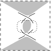
(b)

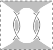
Figure 5. (a) A type (II) bridge gives a bigon of the diagram $D$. (b) More that one type (II) bridge implies the tangle has more than one component.

As we pass from the graphs ${\mathbb{G}_{A}}$, ${\mathbb{G}_{B}}$ to the reduced ones ${\mathbb{G}^{\prime}_{A}}$, ${\mathbb{G}^{\prime}_{B}}$ each bridge loses exactly one of the edges $e^{\prime}$, $e^{\prime\prime}$. The contribution to ${\ell_{\rm ext}}$ from type (I) bridges is half of the number of twist regions in $T$ involved in such bridges.

As for type (II) bridges, if a tangle $T\in\{T_{1},T_{2}\}$ is such that $\Gamma_{A}(T)$ or $\Gamma_{B}(T)$ has more than one bridge of type (II), then $K$ has more than one component. This is illustrated in Figure 5(b). If $\Gamma_{A}(T)$ has more than one bridge of type (II), $T$ must be as shown in the figure, with shaded regions corresponding to vertices of $\Gamma_{A}(T)$, and possibly additional crossings in the white regions of the diagram. Note the four strands in the center region must connect to form one or two distinct link components.

Also observe that there cannot simultaneously be two–crossing twist regions connecting the east side to the west and the north to the south. Hence we may conclude that $T$ contains at most one bridge of type (II).

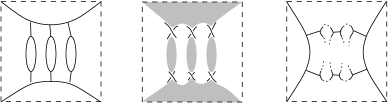
Figure 6. If $\Gamma_{A}(T)$ contains at least three bridges, as at left, then $T$ is as at center, so $\Gamma_{B}(T)$, at right, cannot contain any bridges.

Case 1: Suppose that $b_{A}(T)\geq 3$ or $b_{B}(T)\geq 3$. Without loss of generality, say $b_{A}(T)\geq 3$. Then we claim that $b_{B}(T)=0$. This is illustrated in Figure 6: If $\Gamma_{A}(T)$ contains at least three bridges, then the tangle $T$ must have crossings in the form of the center of that figure. Note no edge of $\Gamma_{B}(T)$ can run through the shaded regions of that figure, else it will correspond to a crossing which would split an interior bridge vertex of $\Gamma_{A}(T)$. Thus any path from the left to the right exterior vertex of $\Gamma_{B}(T)$ must contain at least three edges, so $\Gamma_{B}(T)$ cannot contain any bridges.

Then either there are no type (II) bridges in $\Gamma_{A}(T)$, and then at most ${\mathrm{tw}}(T)/2$ bridges, or there are at most $({\mathrm{tw}}(T)-1)/2$ bridges of type (I) and a single bridge of type (II). In either case, the contribution of $T$ to ${\ell_{\rm ext}}$ is at most

$$b_{A}(T)+b_{B}(T)\>\leq\>\frac{({\mathrm{tw}}(T)-1)}{2}+1\><\>\frac{{\mathrm{tw}}(T)}{2}+2.$$

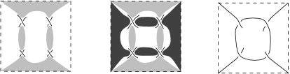
Figure 7. When $b_{A}(T)=b_{B}(T)=2$, $T$ must be as shown in the center. This forces $T$ to have at least two components, as at right.

Case 2: Next, suppose that $b_{A}(T)\leq 2$ and $b_{B}(T)\leq 2$. Then $b_{A}(T)+b_{B}(T)\leq 4$, and the maximum contribution to ${\ell_{\rm ext}}(T)$ occurs when $b_{A}(T)=b_{B}(T)=2$. However, we now show that when $b_{A}(T)=b_{B}(T)=2$, we actually have a link rather than a knot. This is illustrated in Figure 7. If $b_{A}(T)=2$, the tangle diagram must be as in the left of that figure. Similarly, if $b_{B}(T)=2$, the tangle diagram must be as in the left, but rotated 90 degrees. Since edges of $\Gamma_{B}(T)$ cannot pass through the vertices of $\Gamma_{A}(T)$ (shaded regions of the figure), and vice versa, the only possibility is that the tangle $T$ has the form in the center. Here the lighter shaded regions become vertices of $\Gamma_{A}(T)$, and the darker become vertices of $\Gamma_{B}(T)$. But then $T$ must actually have a diagram as on the right of the figure, because closures of the diagram are prime, implying the diagram is prime. Note the tangle must consist of at least two components.

So suppose $b_{A}(T)=2$ and $b_{A}(T)=1$, or vice versa. Then because there is at most one bridge of type (II), $T$ must contain at least two twist regions. Thus

$$b_{A}(T)+b_{B}(T)=3\leq\frac{{\mathrm{tw}}(T)}{2}+2.$$

For strongly alternating tangles, the twist number is additive under tangle addition, which can be seen as follows. Suppose $T_{a}$ and $T_{b}$ are tangles whose sum has diagram $\Delta$. First, since equivalent crossings in a tangle are still equivalent after tangle addition, and tangle addition does not produce more crossings, ${\mathrm{tw}}(\Delta)\leq{\mathrm{tw}}(T_{a})+{\mathrm{tw}}(T_{b})$. Suppose ${\mathrm{tw}}(\Delta)$ is strictly less than ${\mathrm{tw}}(T_{a})+{\mathrm{tw}}(T_{b})$. That means two twist regions in distinct tangles become equivalent under tangle sum. By definition, there exists a simple closed curve $\gamma$ in $\Delta$ meeting just a crossing in $T_{a}$, and just a crossing in $T_{b}$. It must run through the unit square bounding $T_{a}$. Note by parity, $\gamma$ either intersects the north and south edges of the unit square, or the east and west edges. But in the first case, the denominator of the tangle is not prime, and in the second the numerator is not prime, contradicting strongly alternating. Thus the twist number is additive under tangle addition.

The previous inequality therefore implies that

$${\ell_{\rm ext}}(D)\;\leq\;\sum_{i=1,2}(b_{A}(T_{i})+b_{B}(T_{i}))\;\leq\;\frac{{\mathrm{tw}(D)}}{2}+4.$$

∎

Proof of Theorem 1.6.

It is well–known that the Jones polynomial of a link remains invariant under mutation [17]. Thus, for our purposes, we are free to modify $D$ by mutation. After mutation we can assume that the sum of the tangles $T_{1}+\ldots+T_{n}$ is either a strongly alternating tangle, or it splits in the form $T+T^{\prime}$ where each of $T$, $T^{\prime}$ is strongly alternating and $T+T^{\prime}$ is not alternating. In the former case we have a stronger result: Dasbach and Lin [10] have shown that ${\mathrm{tw}(D)}={\left|\beta\right|}+{\left|\beta^{\prime}\right|}$.

So now we assume that $D$ is not alternating. By work of Lickorish and Thistlethwaite [18], $D$ is an adequate diagram; thus the results stated above apply for $K$. By Propositions 1 and 5 of [18] (see also [9]) we have

(2) $$v_{A}+v_{B}=c,$$

where $c:=c(D)$ denotes the crossing number of $D$. Now, recall that every edge of ${\mathbb{G}_{A}}$ or ${\mathbb{G}_{B}}$ that is lost as we pass to ${\mathbb{G}^{\prime}_{A}}$ and ${\mathbb{G}^{\prime}_{B}}$ either comes from a twist region in a tangle, or an edge of an inadmissible bridge. The number of edges lost due to twist regions is $c-t$, where $t={\mathrm{tw}(D)}$. Thus

$$e_{A}+e_{B}-e^{\prime}_{A}-e^{\prime}_{B}\;=\;(c-t)+{\ell_{\rm ext}}.$$

Now by Lemma 5.1, we have

$${\left|\beta\right|}+{\left|\beta^{\prime}\right|} = e^{\prime}_{A}+e^{\prime}_{B}-v_{A}-v_{B}+2$$

$$= (e^{\prime}_{A}+e^{\prime}_{B}-e_{A}-e_{B})+e_{A}+(e_{B}-v_{A}-v_{B})+2$$

$$= -(c-t+{\ell_{\rm ext}})+c+(c-v_{A}-v_{B})+2$$

$$\geq t-{\ell_{\rm ext}}+2\hskip 123.58218pt\mbox{(by (\ref{eqn:lith}))}$$

$$\geq t-\frac{t}{2}-4+2=\frac{t}{2}-2\hskip 72.26999pt\mbox{(by Lemma \ref{lemma:ltop-estimate})}$$

The upper bound on ${\left|\beta\right|}+{\left|\beta^{\prime}\right|}$ was proved in Proposition 4.6 of [12]. ∎

References

- [1] Colin Adams, Waist size for cusps in hyperbolic 3-manifolds II, Preprint.
- [2] by same author, Thrice-punctured spheres in hyperbolic -manifolds, Trans. Amer. Math. Soc. 287 (1985), no. 2, 645–656.
- [3] by same author, Maximal cusps, collars, and systoles in hyperbolic surfaces, Indiana Univ. Math. J. 47 (1998), no. 2, 419–437.
- [4] by same author, Noncompact Fuchsian and quasi-Fuchsian surfaces in hyperbolic 3-manifolds, Algebr. Geom. Topol. 7 (2007), 565–582.
- [5] Colin Adams, Hanna Bennett, Christopher Davis, Michael Jennings, Jennifer Novak, Nicholas Perry, and Eric Schoenfeld, Totally Geodesic Seifert Surfaces in Hyperbolic Knot and Link Complements II, arXiv:math.GT/0411358.
- [6] Ian Agol, The minimal volume orientable hyperbolic 2–cusped 3–manifolds, arXiv:0804.0043.
- [7] by same author, Bounds on exceptional Dehn filling, Geom. Topol. 4 (2000), 431–449 (electronic).
- [8] Ian Agol, Peter A. Storm, and William P. Thurston, Lower bounds on volumes of hyperbolic Haken 3-manifolds, J. Amer. Math. Soc. 20 (2007), no. 4, 1053–1077, with an appendix by Nathan Dunfield.
- [9] Oliver T. Dasbach, David Futer, Efstratia Kalfagianni, Xiao-Song Lin, and Neal W. Stoltzfus, The Jones polynomial and graphs on surfaces, Journal of Combinatorial Theory Ser. B 98 (2008), no. 2, 384–399.
- [10] Oliver T. Dasbach and Xiao-Song Lin, A volumish theorem for the Jones polynomial of alternating knots, Pacific J. Math. 231 (2007), no. 2, 279–291.
- [11] David Futer, Efstratia Kalfagianni, and Jessica S. Purcell, Cusp areas of Farey manifolds and applications to knot theory, arXiv:0808.2716.
- [12] by same author, Dehn filling, volume, and the Jones polynomial, J. Differential Geom. 78 (2008), no. 3, 429–464.
- [13] David Gabai, Robert Meyerhoff, and Peter Milley, Minimum volume cusped hyperbolic three-manifolds, arXiv:0705.4325.
- [14] by same author, Mom technology and volumes of hyperbolic 3–manifolds, arXiv:0606072.
- [15] Marc Lackenby, Word hyperbolic Dehn surgery, Invent. Math. 140 (2000), no. 2, 243–282.
- [16] by same author, The volume of hyperbolic alternating link complements, Proc. London Math. Soc. (3) 88 (2004), no. 1, 204–224, With an appendix by Ian Agol and Dylan Thurston.
- [17] W. B. Raymond Lickorish, An introduction to knot theory, Graduate Texts in Mathematics, vol. 175, Springer-Verlag, New York, 1997.
- [18] W. B. Raymond Lickorish and Morwen B. Thistlethwaite, Some links with nontrivial polynomials and their crossing-numbers, Comment. Math. Helv. 63 (1988), no. 4, 527–539.
- [19] Bruno Martelli and Carlo Petronio, Dehn filling of the “magic” 3-manifold, Comm. Anal. Geom. 14 (2006), no. 5, 969–1026.
- [20] Peter Milley, Source code to check bounds on the volume and cusp area of non– manifolds is available free of charge by e-mail from Milley.
- [21] by same author, Minimum-volume hyperbolic 3-manifolds, arXiv:0809.0346.
- [22] John Morgan and Gang Tian, Ricci flow and the Poincaré conjecture, Clay Mathematics Monographs, vol. 3, American Mathematical Society, Providence, RI, 2007.
- [23] John W. Morgan and Hyman Bass (eds.), The Smith conjecture, Pure and Applied Mathematics, vol. 112, Academic Press Inc., Orlando, FL, 1984, Papers presented at the symposium held at Columbia University, New York, 1979.
- [24] Harriet Moser, Proving a manifold to be hyperbolic once it has been approximated to be so, Ph.D. thesis, Columbia University, 2004.
- [25] William P. Thurston, The geometry and topology of three-manifolds, Princeton Univ. Math. Dept. Notes, 1979.
- [26] by same author, Three-dimensional manifolds, Kleinian groups and hyperbolic geometry, Bull. Amer. Math. Soc. (N.S.) 6 (1982), no. 3, 357–381.
- [27] Friedhelm Waldhausen, On irreducible -manifolds which are sufficiently large, Ann. of Math. (2) 87 (1968), 56–88.