RIKEN-TH-125 April, 2008

UT-08-07

Gauge Invariant Overlaps for Classical Solutions

in Open String Field Theory

Teruhiko Kawano^a, Isao Kishimoto^b and Tomohiko Takahashi^c

^a) Department of Physics, University of Tokyo, Hongo, Tokyo 113-0033, Japan
^b) Theoretical Physics Laboratory, RIKEN, Wako 351-0198, Japan
^c) Department of Physics, Nara Women’s University, Nara 630-8506, Japan

We calculate gauge invariant observables for Schnabl’s solution with analytic method and with the level truncation approximation. We also compute them for the numerical solution initially obtained by Sen and Zwiebach in the level truncation approximation to compare with the one for Schnabl’s solution. The results are consistent with the expectation that they may be gauge equivalent. We briefly discuss the gauge invariant observables and the action for a marginal solution with a nonsingular current.

1 Introduction

After the advent of the paper [1], tachyon condensation has been studied in Witten’s bosonic open string field theory. They used the level truncation approximation [2] to obtain a classical solution numerically and obtained its vacuum energy giving 99% of the D-brane tension. The approximation have been improved soon later to the higher level [3, 4].

More recently, Schnabl has discovered an analytic classical solution in the open string field theory. The analytic solution also describes tachyon condensation, because its vacuum energy is exactly equal to the D25-brane tension [5, 6, 7], and the BRST cohomology around it is trivial [8], which implies that there are no physical degrees of freedom of open strings perturbatively, as conjectured by Sen [9, 10, 11].

We thus have two classical solutions of the open string field theory; the numerical one and the analytical one. Therefore, it seems natural to ask the relation between them. Since they give the same vacuum energy equal to the D-brane tension, one likely suspects that they may be gauge equivalent solutions. In order to confirm the expectation, one needs gauge invariant observables to compare their values for these two solutions.

Zwiebach introduced the couplings of a single on-shell closed string state with open string field into the open string field theory in a gauge invariant fashion [12]. In fact, it has been shown [13, 14] that the couplings exactly give the disk amplitudes with two closed strings and the ones with one closed string and two open strings. They have also been used to discuss the closed string degrees of freedom in vacuum string field theory [15]. The gauge invariance of the coupling with the closed string tachyon was reassured [16] in terms of the oscillator formalism. Hashimoto and Itzhaki also emphasized that they are also gauge invariant observables [16].

In this paper, the gauge invariant observables will be called gauge invariant overlaps to distinguish with general gauge invariant observables.

In this paper, we will calculate the gauge invariant overlaps for Schnabl’s solution $\Psi_{\lambda}$ with the parameter $\lambda$ analytically in the sliver frame and numerically with the level truncation. The results on the vacuum energy of the solution $\Psi_{\lambda}$ imply that only the solution with $\lambda=1$ cannot be gauged away and is thus physically non-trivial, while the rest is all trivial. The analytical results on the gauge invariant overlaps for the solution $\Psi_{\lambda}$ are consistent with the ones of the vacuum energy. There however exist subtleties in the evaluation, and thus we will confirm the results numerically in the level truncation approximation, as done for the vacuum energy in [5, 17]

We will also compute the gauge invariant overlaps for the numerical solution $\Psi_{\rm N}$ in [1, 3, 4] with the level truncation to compare with the results for Schnabl’s solution with $\lambda=1$, and we will show that the comparison is consistent with the expectation that they are gauge equivalent.

Furthermore, we will briefly report our results on the gauge invariant overlaps for a marginal solution with a nonsingular current $i\partial X^{+}$ in [18, 19] and that it vanishes as an evaluation of the action.

This paper is organized as follows. In the next section, we will give a brief review on the gauge invariant overlaps of the on-shell closed string states and make a few comments on the relation to the open-closed string vertex. In §3, we will evaluate the gauge invariant overlaps for Schnabl’s solution $\Psi_{\lambda}$, both analytically and numerically. In §4, we will give the results for the numerical solution $\Psi_{\rm N}$. In §5, we will discuss the gauge invariant for the marginal solution analytically. In §6, we give summary and discussions on our results. In appendices, we will explicitly give a few examples of the gauge invariant overlaps and the Shapiro-Thorn’s open-closed string vertex, and will explain technical details on our computations.

2 Gauge Invariant Overlaps

In Witten’s bosonic open string field theory, the action is given by

$$S[\Psi] = -{1\over g^{2}}\left({1\over 2}\langle\Psi,Q_{\rm B}\Psi\rangle+{1\over 3}\langle\Psi,\Psi*\Psi\rangle\right),$$ (2.1)

which is left invariant under the gauge transformation

$$\delta_{\Lambda}\Psi=Q_{\rm B}\Lambda+\Psi*\Lambda-\Lambda*\Psi$$ (2.2)

with a gauge ‘parameter’ $\Lambda$. It was discussed in [12, 16, 15] that

$${\cal O}_{V}(\Psi) = \langle V(i)f_{\cal I}[\Psi]\rangle\,,~{}~{}~{}~{}~{}f_{\cal I}(z)\equiv\frac{2z}{1-z^{2}}\,.$$ (2.3)

is gauge invariant under (2.2), where the CFT correlator is defined on the upper half plane, and will be called a gauge invariant overlap in this paper. The operator $V(i)$ is inserted at the midpoint of the string field $\Psi$ and is a primary field of conformal dimension $(0,0)$ and the ghost number two. The holomorphic function $f_{\cal I}(z)$ maps the unit half disk to the upper half plane. Since the identity state $\langle{\cal I}|$ may be defined by $\langle{\cal I}|\phi\rangle=\langle f_{\cal I}[\phi(0)]\rangle$, one may rewrite the gauge invariant overlap ${\cal O}_{V}(\Psi)$ as

$${\cal O}_{V}(\Psi) = \langle{\cal I}|V(i)|\Psi\rangle=\langle\Phi_{V},\Psi\rangle\,,$$ (2.4)

with the definition

$${}|\Phi_{V}\rangle \equiv V(i)|{\cal I}\rangle.$$ (2.5)

A few examples of $|\Phi_{V}\rangle$ in terms of the oscillators are explicitly given in appendix A. Because $V(i)$ is inserted at the midpoint of the identity state $|{\cal I}\rangle$, one can see that $\langle\Phi_{V},\Psi*\Lambda\rangle=\langle\Phi_{V},\Lambda*\Psi\rangle$, or in other words,

$${\cal O}_{V}(\Psi*\Lambda)={\cal O}_{V}(\Lambda*\Psi),$$ (2.6)

at least naïvely. Therefore, by requiring $\Phi_{V}$ to satisfy that $Q_{\rm{B}}|\Phi_{V}\rangle=0$, one can finds that ${\cal O}_{V}(\delta_{\Lambda}\Psi)=0$. One thus obtains the gauge invariant observables ${\cal O}_{V}(\Psi)$. In particular, note that it vanishes for pure gauge solutions

$${\cal O}_{V}(e^{-\Lambda}Q_{\rm B}e^{\Lambda})=\int_{0}^{1}dt\,{\cal O}_{V}(e^{-t\Lambda}*Q_{\rm B}\Lambda*e^{t\Lambda})={\cal O}_{V}(Q_{\rm B}\Lambda)=-\langle Q_{\rm B}\Phi_{V},\Lambda\rangle=0\,.$$ (2.7)

Incidentally, it could be helpful to rewrite the gauge invariant overlap ${\cal O}_{V}(\Psi)$ by using open-closed string vertex, which maps states in the closed string Hilbert space to the ones in the open string one. Let us consider the Shapiro-Thorn vertex $\langle\hat{\gamma}(1_{\rm c},2)|$ given in [20], which is defined with the conformal maps $h_{1}(w)=-i(w-1)/(w+1)$ and $h_{2}(w)=(w-1/w)/2$ by the CFT correlator on the upper half plane as

$$\langle\hat{\gamma}(1_{\rm c},2)|\phi_{\rm c}\rangle_{1_{\rm c}}|\psi\rangle_{2}=\langle h_{1}[\phi_{\rm c}(0,0)]h_{2}[\psi(0)]\rangle,$$ (2.8)

where $|\phi_{\rm c}\rangle_{1_{\rm c}}=\phi_{\rm c}(0,0)|0\rangle_{1_{\rm c}}$ is in the closed string Hilbert space and $|\psi\rangle_{2}=\psi(0)|0\rangle_{2}$ is in the open string one. These conformal maps are depicted in Figure 1 and 2. (See, appendix B for detail.)

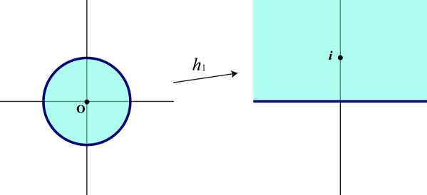
Figure 1: The conformal map $h_{1}$ in the definition of the Shapiro-Thorn vertex. The map $h_{1}$ transforms a unit disc to the upper half plane. The center at the origin, the insertion point of a closed string is mapped to $i$.

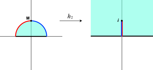
Figure 2: The conformal map $h_{2}$ in the definition of the Shapiro-Thorn vertex. The map $h_{2}$ transforms a unit half disc to the upper half plane. The open string midpoint $i$ is also mapped to $i$. The left half and the right half of the open string are identified on the mapped plane.

Since $h_{1}(0)=i$ and $h_{2}(w)=I\circ f_{\cal I}(w)$, where $I(z)=-1/z$ is the inversion map, one obtains

$$\langle\hat{\gamma}(1_{\rm c},2)|V_{\rm c}\rangle_{1_{\rm c}}|\psi\rangle_{2} = \langle h_{1}[V_{\rm c}(0,0)]h_{2}[\psi(0)]\rangle=\langle I\circ h_{1}[V_{\rm c}(0,0)]\,f_{\cal I}[\psi(0)]\rangle$$ (2.9)

$$= \langle V_{\rm c}(i,-i)\,f_{\cal I}[\psi(0)]\rangle~{}~{}~{}~{}~{}~{}$$

for a primary field $V_{\rm c}(z,\bar{z})$ of conformal dimension $(0,0)$ and the ghost number two. By identifying $V(i)$ in (2.3) with $V_{\rm c}(i,-i)$, one finds that

$${\cal O}_{V}(\Psi) = \langle\hat{\gamma}(1_{\rm c},2)|V_{\rm c}\rangle_{1_{\rm c}}|\Psi\rangle_{2}\,.$$ (2.10)

It means that $|\Phi_{V}\rangle$ in (2.5) can be given by $|V_{\rm c}\rangle=V_{\rm{c}}(0,0)|0\rangle$:

$${}|\Phi_{V}\rangle_{3}=V(i)|{\cal I}\rangle_{3}=\langle\hat{\gamma}(1_{\rm c},2)|V_{\rm c}\rangle_{1_{\rm c}}|R(2,3)\rangle\,,$$ (2.11)

where $|R(2,3)\rangle$ is the reflector and can be used to define the BPZ conjugation. Using the BRST invariance of the string vertices $\langle\hat{\gamma}(1_{\rm c},2)|$ and $|R(2,3)\rangle$

$$\langle\hat{\gamma}(1_{\rm c},2)|(Q_{\rm B}^{(1)}+\bar{Q}_{\rm B}^{(1)}+Q_{\rm B}^{(2)})=0\,,~{}~{}~{}~{}(Q_{\rm B}^{(2)}+Q_{\rm B}^{(3)})|R(2,3)\rangle=0\,,$$ (2.12)

one can show that $(Q_{\rm B}+\bar{Q}_{\rm B})|V_{\rm c}\rangle=0$ means $Q_{\rm B}|\Phi_{V}\rangle$=0. The other condition (2.6), required for the gauge invariance of the overlaps, can be proven by the generalized gluing and re-smoothing theorem (B.3). Therefore, if a primary field $V_{\rm c}(z,\bar{z})$ of conformal dimension $(0,0)$ and the ghost number two is BRST invariant, it yields a gauge invariant overlap by $\langle\hat{\gamma}(1_{\rm c},2)|$ via (2.10). Therefore, it may be natural to call $\left|\Phi_{V}\right>$ an on-shell closed string state in the open string Hilbert space. In particular, when $V_{\rm c}(z,\bar{z})$ can be put in the form $V_{\rm c}(z,\bar{z})=c(z)\bar{c}(\bar{z})V_{\rm m}(z,\bar{z})$, where $V_{\rm m}(z,\bar{z})$ is in the matter sector, the BRST invariance is guaranteed, if $V_{\rm m}(z,\bar{z})$ is a primary field of conformal dimension $(1,1)$.

For later convenience, it is useful to understand that on-shell closed string states are left invariant by the transformation generated by $K_{n}=L_{n}-(-1)^{n}L_{-n}$, where $L_{n}$ is the total Virasoro operator with the central charge zero. In fact, the requirement that $V_{\rm c}(z,\bar{z})$ be a primary field of dimension $(0,0)$, $\Phi_{V}$ means that

$$K_{n}|\Phi_{V}\rangle=0\,,~{}~{}~{}~{}~{}~{}~{}(n=1,2,3,\cdots).$$ (2.13)

Because $K_{n}$ is odd under the BPZ conjugation, the $K_{n}$ invariance (2.13) of on-shell closed string states means that ${\cal O}_{V}(\Psi)$ is invariant under the transformation $\Psi\to{}e^{\sum_{n}v_{n}K_{n}}\Psi$ on an open string field $\Psi$;

$${\cal O}_{V}(e^{\sum_{n}v_{n}K_{n}}\Psi)={\cal O}_{V}(\Psi)$$ (2.14)

for any constants $v_{n}$. It may be regarded as a part of the gauge symmetry [21, 22]. Moreover, if we take a form $V_{\rm c}(z,\bar{z})=c(z)\bar{c}(\bar{z})V_{\rm m}(z,\bar{z})$, where $V_{\rm m}(z,\bar{z})$ is a primary field of conformal dimension $(1,1)$, $\left|\Phi_{V}\right>$ satisfies

$$K_{2m-1}^{({\rm m})}|\Phi_{V}\rangle=0\,,~{}~{}~{}(K_{2m}^{({\rm m})}-3(-1)^{m}m)|\Phi_{V}\rangle=0\,,~{}~{}~{}(m=1,2,3,\cdots)$$ (2.15)

where $K_{n}^{({\rm m})}\equiv L_{n}^{({\rm m})}-(-1)^{n}L_{-n}^{({\rm m})}$ for the matter Virasoro operator $L^{({\rm m})}_{n}$ and also

$$K_{2m-1}^{({\rm gh})}|\Phi_{V}\rangle=0\,,~{}~{}~{}~{}~{}~{}(K_{2m}^{({\rm gh})}+3(-1)^{m}m)|\Phi_{V}\rangle=0\,,~{}~{}~{}~{}~{}~{}~{}(m=1,2,3,\cdots)\,,$$ (2.16)

where $K_{n}^{({\rm gh})}\equiv L_{n}^{({\rm gh})}-(-1)^{n}L_{-n}^{({\rm gh})}$ for the ghost Virasoro operator $L^{({\rm gh})}_{n}$. The above relations (2.13), (2.15) and (2.16) can be derived from more general relations given in (B.35) and (B.36).

In this paper, we will restrict ourselves to consider on-shell closed string states of the form

$$\left|\Phi_{V}\right> = \sum_{m,n}\zeta_{mn}c(i)V_{m}(i)c(-i)V_{n}(-i)|{\cal I}\rangle,$$ (2.17)

where $\zeta_{mn}$ is the polarization constant with $V_{m}(z)$ a matter primary field on the doubling of the upper half plane.

3 Gauge Invariant Overlaps for Schnabl’s Solution

Let us begin with a brief review on the analytic solution $\Psi_{\lambda}$ discovered by Schnabl in [5]. Schnabl has found the sliver frame very useful to obtain the solution. In the frame, a primary field $\tilde{\phi}(\tilde{z})$ of conformal dimension $h$ is related by the conformal transformation $\tilde{z}=\arctan z$ to the usual one $\phi(z)$ on the canonical upper half plane as $\tilde{\phi}(\tilde{z})=(1+z^{2})^{h}\phi(z)$. The field $\tilde{\phi}(\tilde{z})$ is expanded in terms of the oscillators $\tilde{\phi}_{n}$ as $\tilde{\phi}(\tilde{z})=\sum_{n}\tilde{\phi}_{n}{\tilde{z}}^{-n-h}$. In this paper, the tilde $\tilde{\ }$ refers to the sliver frame, as in [5]. In particular, the operators $\hat{\cal L}\equiv{\cal L}_{0}+{\cal L}_{0}^{\dagger}$, ${\hat{\cal B}}\equiv{\cal B}_{0}+{\cal B}_{0}^{\dagger}$ will be often used in this paper, where ${\cal L}_{0}=\tilde{L}_{0}$ and ${\cal B}_{0}=\tilde{b}_{0}$ are zero modes of the total energy momentum tensor and $b$-ghost field, respectively.

Making use of the oscillators, Schnabl gave one parameter of solutions

$$\Psi_{\lambda} = \sum_{n=0}^{\infty}\sum_{p\geq-1,\,p:{\rm odd}}{(-1)^{n}\pi^{p}\over n!\,2^{n+2p+1}}f_{n+p+1}(\lambda)\hat{\cal L}^{n}\tilde{c}_{-p}|0\rangle$$ (3.1)

$$+\sum_{n=0}^{\infty}\sum_{p,q\geq-1,\,p+q:{\rm odd}}{(-1)^{n+q}\pi^{p+q}\over n!\,2^{n+2(p+q)+3}}f_{n+p+q+2}(\lambda)\hat{\cal B}\hat{\cal L}^{n}\tilde{c}_{-p}\tilde{c}_{-q}|0\rangle\,,$$

parametrized by $\lambda$, where the function $f_{n}(\lambda)$ is defined by

$$f_{n}(\lambda) = \left\{\begin{array}[tb]{lc}B_{n}&(\lambda=1),\\ -n\lambda\,{\rm Li}_{1-n}(\lambda)-\delta_{n,1}\lambda&(\lambda\neq 1),\end{array}\right.$$ (3.4)

with the Bernoulli number $B_{n}$ and the polylogarithmic function ${\rm Li}_{n}(z)$. The functions $f_{n}(\lambda)$ can also be organized in the generating function

$$\frac{\lambda z}{\lambda e^{z}-1} = \sum_{n=0}^{\infty}\frac{f_{n}(\lambda)}{n!}z^{n}.$$ (3.5)

In order to put the solution (3.1) in a somewhat simpler form, it is useful to introduce string fields

$$\psi_{r} \equiv {2\over\pi}\hat{U}_{r+2}\!\left[-\frac{1}{\pi}\hat{\cal B}\tilde{c}(\frac{\pi r}{4})\tilde{c}(-\frac{\pi r}{4})+\frac{1}{2}(\tilde{c}(-\frac{\pi r}{4})+\tilde{c}(\frac{\pi r}{4}))\right]\!|0\rangle$$

$$= \!\!\underset{p:{\rm odd}}{\sum_{n\geq 0;p\geq-1}}\!\frac{(-1)^{n}\pi^{p}}{n!2^{n+2p+1}}r^{n+p+1}\hat{\cal L}^{n}\tilde{c}_{-p}|0\rangle+\!\!\underset{p+q:{\rm odd}}{\sum_{n\geq 0;p,q\geq-1}}\!\frac{(-1)^{n+q}\pi^{p+q}}{n!2^{n+2p+2q+3}}r^{n+p+q+2}\hat{\cal B}\hat{\cal L}^{n}\tilde{c}_{-p}\tilde{c}_{-q}|0\rangle,$$

where

$$\hat{U}_{r}\equiv U_{r}^{\dagger}U_{r}=e^{-\frac{r-2}{2}\hat{\cal L}}$$ (3.7)

with $U_{r}=(2/r)^{{\cal L}_{0}}$. They can be used to give a wedge state $\langle r|=\langle 0|\hat{U}_{r}=\langle 0|U_{r}$, which is a surface state defined by the conformal map $f_{r}(z)=\tan\left((2/r)\arctan z\right)$. Using the generating function (3.5) and the string fields $\psi_{r}$, one can see that the solution $\Psi_{\lambda}$ is given by

$$\Psi_{\lambda} = \frac{\lambda\partial_{r}}{\lambda e^{\partial_{r}}-1}\psi_{r}|_{r=0}=\sum_{k=0}^{\infty}\frac{f_{k}(\lambda)}{k!}\partial_{r}^{k}\psi_{r}|_{r=0}.$$ (3.8)

Upon expanding the right hand side of (3.8) in terms of the derivative $\partial_{r}$, one can see that it starts with 1 for $\lambda=1$, otherwise it starts with $\lambda/(\lambda-1)\partial_{r}$. Therefore, for $\lambda\not=1$, by expanding (3.8) formally in terms of $\lambda$, one finds that

$$\Psi_{\lambda\neq 1} = -\lambda\sum_{n=0}^{\infty}\lambda^{n}e^{n\partial_{r}}\partial_{r}\psi_{r}|_{r=0}=-\sum_{n=0}^{\infty}\lambda^{n+1}\partial_{r}\psi_{r}|_{r=n},$$ (3.9)

which certainly starts with the first derivative $\partial_{r}$. It was in this form (3.9) that the solution $\Psi_{\lambda\neq 1}$ was shown in [5] to satisfy the equation of motion order by order in $\lambda$.

For $\lambda=1$, exploiting the Euler-Maclaurin formula, Schnabl has discussed that the solution has the expansion

$$\Psi_{\lambda=1} = \lim_{N\to\infty}\left(\psi_{N+1}-\sum_{n=0}^{N}\partial_{r}\psi_{r}|_{r=n}\right).$$ (3.10)

The first term $\lim_{N\to\infty}\psi_{N+1}$ is called the phantom term and gives finite contributions to the classical action [5] for the solution. The solution wouldn’t satisfy the equation of motion $\langle\Psi_{\lambda=1},(Q_{\rm B}\Psi_{\lambda=1}+\Psi_{\lambda=1}*\Psi_{\lambda=1})\rangle=0$ in the ‘strong’ sense without the phantom term [6, 7].

In the next two subsections, we will evaluate the gauge invariant overlap (2.4) for the solution $\Psi_{\lambda}$ in two ways; analytically in the sliver frame and numerically with the conventional level truncation.

3.1 Analytic Evaluation in the Sliver Frame

Let us first evaluate the gauge invariant overlap ${\cal O}_{V}(\Psi_{\lambda})$ analytically in the sliver frame. Since one can verify that

$$U_{1}^{\dagger}={\rm bpz}(U_{f_{\cal I}})=U^{-1}_{I\circ f_{\cal I}\circ I},~{}~{}~{}~{}\phi(z)U_{1}^{\dagger}=U_{1}^{\dagger}(I\circ f_{\cal I}\circ I\circ\phi(z)),$$ (3.11)

$$f_{\cal I}(z)=\frac{2z}{1-z^{2}}\,,~{}~{}~{}~{}I(z)=-\frac{1}{z}\,,$$ (3.12)

by using them, one finds that

$$\hat{U}_{1}^{-1}\phi(e^{i\theta})\hat{U}_{1}=(\cos(it+\frac{\pi}{4}))^{2h}\,\tilde{\phi}(it)\,,~{}~{}~{}~{}e^{i\theta}=\tan(it+\frac{\pi}{4})\,,$$ (3.13)

for a primary field $\phi$ of conformal dimension $h$.

Using (3.13), one can rewrite the on-shell closed string state (2.17) as

$$\Phi_{V} = \sum_{m,n}\zeta_{mn}\hat{U}_{1}\tilde{c}(i\infty)\tilde{V}_{m}(i\infty)\tilde{c}(-i\infty)\tilde{V}_{n}(-i\infty)|0\rangle$$ (3.14)

with the operators in the sliver frame, and one may regularize it by replacing $\pm i\infty$ by $\pm iM$ in the arguments of the fields as

$$\Phi_{V,M} = \sum_{m,n}\zeta_{mn}\hat{U}_{1}\tilde{c}(iM)\tilde{V}_{m}(iM)\tilde{c}(-iM)\tilde{V}_{n}(-iM)|0\rangle,$$ (3.15)

to make well-defined our calculation of the gauge invariant overlap (2.4).

In order to estimate the gauge invariant overlap (2.4) for the analytic solution $\Psi_{\lambda}$, essentially one needs to calculate the inner product $\langle\Phi_{V,M},\psi_{r}\rangle$. However, instead of it, since $\left<{\Phi_{V,M},\psi_{r}}\right>=\langle{\cal I}|\Phi_{V,M}*\psi_{r}\rangle=\langle{\cal I}|\psi_{r}*\Phi_{V,M}\rangle$, one may compute $\langle{\cal I}|\Phi_{V,M}*\psi_{r}\rangle$ or $\langle{\cal I}|\psi_{r}*\Phi_{V,M}\rangle$.

The sliver frame facilitates the calculation of the star products of string fields, and in particular, one finds [5] that

$$\hat{U}_{r}\tilde{\phi}_{1}(\tilde{x}_{1}){\small\cdots}\tilde{\phi}_{n}(\tilde{x}_{n})|0\rangle*\hat{U}_{s}\tilde{\psi}_{1}(\tilde{y}_{1}){\small\cdots}\tilde{\psi}_{m}(\tilde{y}_{m})|0\rangle=\hat{U}_{r+s-1}\tilde{\phi}_{1}(\tilde{x}_{1}^{\prime}){\small\cdots}\tilde{\phi}_{n}(\tilde{x}_{n}^{\prime})\tilde{\psi}_{1}(\tilde{y}_{1}^{\prime}){\small\cdots}\tilde{\psi}_{m}(\tilde{y}_{m}^{\prime})|0\rangle.$$

(3.16)

Note that the coordinates on the right hand side are shifted as $\tilde{x}_{i}^{\prime}=\tilde{x}_{i}+{\pi\over 4}(s-1),\tilde{y}_{j}^{\prime}=\tilde{y}_{j}-{\pi\over 4}(r-1)$. Since the operators

$$B^{R}_{1}=\int_{+i\infty-{\pi\over 4}}^{-i\infty-{\pi\over 4}}{d\tilde{z}\over 2\pi{i}}\tilde{b}(\tilde{z}),\qquad B^{L}_{1}=\int_{-i\infty+{\pi\over 4}}^{+i\infty+{\pi\over 4}}{d\tilde{z}\over 2\pi{i}}\tilde{b}(\tilde{z})$$ (3.17)

act on the right and the left half-string, they satisfy

$$\left(B^{R}_{1}\Psi_{1}\right)*\Psi_{2}=-(-)^{|\Psi_{1}|}\Psi_{1}*\left(B^{L}_{1}\Psi_{2}\right),$$ (3.18)

$$B^{L}_{1}\left(\Psi_{1}*\Psi_{2}\right)=\left(B^{L}_{1}\Psi_{1}\right)*\Psi_{2},\qquad B^{R}_{1}\left(\Psi_{1}*\Psi_{2}\right)=(-)^{|\Psi_{1}|}\Psi_{1}*\left(B^{R}_{1}\Psi_{2}\right).$$ (3.19)

Therefore, using the above formulae (3.18), (3.19) and noting that

$$B^{R}_{1}={1\over 2}B_{1}-{1\over\pi}\hat{\cal B},\qquad B^{L}_{1}={1\over 2}B_{1}+{1\over\pi}\hat{\cal B},$$ (3.20)

one can verify the formulae

$$(\hat{\cal B}\Psi_{1})*\Psi_{2}=\hat{\cal B}(\Psi_{1}*\Psi_{2})+(-1)^{|\Psi_{1}|}\frac{\pi}{2}\Psi_{1}*B_{1}\Psi_{2}\,,$$ (3.21)

$$\Psi_{1}*(\hat{\cal B}\Psi_{2})=(-1)^{|\Psi_{1}|}\hat{\cal B}(\Psi_{1}*\Psi_{2})-(-1)^{|\Psi_{1}|}\frac{\pi}{2}(B_{1}\Psi_{1})*\Psi_{2}\,,$$ (3.22)

where $B_{1}=\tilde{b}_{-1}=b_{1}+b_{-1}$. Using them and the formula (3.16), one finds that the star products $\Phi_{V,M}*\psi_{r}$ and $\psi_{r}*\Phi_{V,M}$ are given by

$$\Phi_{V,M}*\psi_{r}=\frac{1}{\pi}\sum_{m,n}\zeta_{mn}\hat{U}_{r+2}\biggl{(}\!\tilde{c}\tilde{V}_{m}(iM+\frac{\pi}{4}(r+1))\tilde{c}\tilde{V}_{n}(-iM+\frac{\pi}{4}(r+1))\!\left(\tilde{c}(-\frac{\pi}{4}r)+\tilde{c}(\frac{\pi}{4}r)\right)$$

$$~{}~{}~{}~{}~{}~{}~{}~{}~{}~{}~{}~{}~{}~{}~{}+\bigl{(}\tilde{V}_{m}(iM+\frac{\pi}{4}(r+1))\tilde{c}\tilde{V}_{n}(-iM+\frac{\pi}{4}(r+1))$$ (3.23)

$$~{}~{}~{}~{}~{}~{}~{}~{}~{}~{}~{}~{}~{}~{}~{}-\tilde{c}\tilde{V}_{m}(iM+\frac{\pi}{4}(r+1))\tilde{V}_{n}(-iM+\frac{\pi}{4}(r+1))\bigr{)}\tilde{c}(\frac{\pi}{4}r)\tilde{c}(-\frac{\pi}{4}r)$$

$$~{}~{}~{}~{}~{}~{}~{}~{}~{}~{}~{}~{}~{}~{}~{}-\frac{2}{\pi}\hat{\cal B}\tilde{c}\tilde{V}_{m}(iM+\frac{\pi}{4}(r+1))\tilde{c}\tilde{V}_{n}(-iM+\frac{\pi}{4}(r+1))\tilde{c}(\frac{\pi}{4}r)\tilde{c}(-\frac{\pi}{4}r)\biggr{)}|0\rangle,$$

and

$$\psi_{r}*\Phi_{V,M}=\frac{1}{\pi}\sum_{m,n}\zeta_{mn}\hat{U}_{r+2}\biggl{(}\!\tilde{c}\tilde{V}_{m}(iM-\frac{\pi}{4}(r+1))\tilde{c}\tilde{V}_{m}(-iM-\frac{\pi}{4}(r+1))\!\left(\tilde{c}(-\frac{\pi}{4}r)+\tilde{c}(\frac{\pi}{4}r)\right)$$

$$~{}~{}~{}~{}~{}~{}~{}~{}~{}~{}~{}~{}~{}~{}~{}-\bigl{(}\tilde{V}_{m}(iM-\frac{\pi}{4}(r+1))\tilde{c}\tilde{V}_{m}(-iM-\frac{\pi}{4}(r+1))$$ (3.24)

$$~{}~{}~{}~{}~{}~{}~{}~{}~{}~{}~{}~{}~{}~{}~{}-\tilde{c}\tilde{V}_{m}(iM-\frac{\pi}{4}(r+1))\tilde{V}_{m}(-iM-\frac{\pi}{4}(r+1))\bigr{)}\tilde{c}(\frac{\pi}{4}r)\tilde{c}(-\frac{\pi}{4}r)$$

$$~{}~{}~{}~{}~{}~{}~{}~{}~{}~{}~{}~{}~{}~{}~{}-\frac{2}{\pi}\hat{\cal B}\tilde{c}\tilde{V}_{m}(iM-\frac{\pi}{4}(r+1))\tilde{c}\tilde{V}_{m}(-iM-\frac{\pi}{4}(r+1))\tilde{c}(\frac{\pi}{4}r)\tilde{c}(-\frac{\pi}{4}r)\biggr{)}|0\rangle,$$

respectively.

Furthermore, substituting the above results into $\langle{\cal I}|\Phi_{V,M}*\psi_{r}\rangle$ and $\langle{\cal I}|\psi_{r}*\Phi_{V,M}\rangle$ and using the relations

$$\langle{\cal I}|\hat{U}_{r+2}=\langle 0|U_{r+1}\,,~{}~{}~{}\langle{\cal I}|\hat{U}_{r+2}\hat{\cal B}=\frac{2}{r+1}\langle 0|U_{r+1}{\cal B}_{0},$$ (3.25)

one finds that $\langle{\cal I}|\Phi_{V,M}*\psi_{r}\rangle$ and $\langle{\cal I}|\psi_{r}*\Phi_{V,M}\rangle$ give the same results

$$\langle\Phi_{V,M},\psi_{r}\rangle=\langle{\cal I}|\Phi_{V,M}*\psi_{r}\rangle=\langle{\cal I}|\psi_{r}*\Phi_{V,M}\rangle$$

$$=\frac{1}{2\pi}\sum_{m,n}\zeta_{mn}\,{}_{\rm mat}\langle 0|\tilde{V}_{m}(\frac{2iM}{r+1}\pm\frac{\pi}{2})\tilde{V}_{m}(\frac{-2iM}{r+1}\pm\frac{\pi}{2})|0\rangle_{\rm mat}$$

$$~{}~{}\times\biggl{(}-\frac{4iM}{\pi}{}_{bc}\langle 0|\left(\tilde{c}(\frac{-2iM}{r+1}\pm\frac{\pi}{2})+\tilde{c}(\frac{2iM}{r+1}\pm\frac{\pi}{2})\right)\tilde{c}(\frac{\pi r}{2(r+1)})\tilde{c}(\frac{-\pi r}{2(r+1)})|0\rangle_{bc}$$

$$~{}~{}~{}~{}~{}~{}~{}+{}_{bc}\langle 0|\tilde{c}(\frac{2iM}{r+1}\pm\frac{\pi}{2})\tilde{c}(\frac{-2iM}{r+1}\pm\frac{\pi}{2})\left(\tilde{c}(\frac{-\pi r}{2(r+1)})+\tilde{c}(\frac{\pi r}{2(r+1)})\right)|0\rangle_{bc}\biggr{)}$$

$$=\frac{C_{V}}{2\pi i}\left(\sinh\frac{4M}{r+1}-\frac{4M}{\pi}\sin\frac{\pi}{r+1}\right)\left(\cosh\frac{4M}{r+1}-\cos\frac{\pi}{r+1}\right)\left(\sinh\frac{4M}{r+1}\right)^{-2},$$

(3.26)

where the factor $C_{V}$ is given by

$$C_{V} = {}_{\rm mat}\langle 0|0\rangle_{\rm mat}\sum_{m,n}\zeta_{mn}v_{mn}.$$ (3.27)

The constants $v_{mn}$ are the metric appearing in the OPE of the matter primary fields $V_{m}(z)$ of conformal dimension one as

$$V_{m}(y)V_{n}(z) \sim \frac{v_{mn}}{(y-z)^{2}}+{\rm finite}\,.~{}~{}~{}~{}~{}(y\to z)$$ (3.28)

By taking the limit $M\to+\infty$ in (3.26), one obtains

$$\langle\Phi_{V},\psi_{r}\rangle=\lim_{M\to+\infty}\langle\Phi_{V,M},\psi_{r}\rangle=\frac{C_{V}}{2\pi i}\,.$$ (3.29)

It is interesting to note that $\langle\Phi_{V},\psi_{r}\rangle$ is independent of $r$, and thus one can see that $\partial_{r}\langle\Phi_{V},\psi_{r}\rangle=0$. It in turn means that

$${\cal O}_{V}(\Psi_{\lambda}) = \sum_{k=0}^{\infty}\frac{f_{k}(\lambda)}{k!}\partial_{r}^{k}\langle\Phi_{V},\psi_{r}\rangle|_{r=0}=f_{0}(\lambda)\langle\Phi_{V},\psi_{0}\rangle$$ (3.32)

$$= \left\{\begin{array}[tb]{lc}\displaystyle\frac{C_{V}}{2\pi i}&(\lambda=1),\\ \displaystyle 0&(\lambda\neq 1).\end{array}\right.$$

Namely, the value can be nonzero only for $\lambda=1$. It seems that this nonzero value only comes from the inner product with the phantom term $\psi_{N+1}$, if one uses the expression given in (3.10). From this viewpoint, we should not take the limit $N\to\infty$ first because the inner product vanishes for finite $M$ in (3.26); $\lim_{N\to\infty}\langle\Phi_{V,M},\psi_{N+1}\rangle=0$, which means that the order of the two limits isn’t interchangeable

$$\lim_{N\to\infty}\biggl{(}\lim_{M\to+\infty}\langle\Phi_{V,M},\psi_{N+1}\rangle\biggr{)} \neq \lim_{M\to+\infty}\biggl{(}\lim_{N\to\infty}\langle\Phi_{V,M},\psi_{N+1}\rangle\biggr{)}\,.$$ (3.33)

The order on the left hand side is consistent with our evaluation with the expression (3.8) to yield the result (3.32). Rearranging the terms in the expression (3.10), one obtains

$$\Psi_{\lambda=1} = \psi_{0}+\sum_{n=0}^{\infty}\left(\psi_{n+1}-\psi_{n}-\partial_{r}\psi_{r}|_{r=n}\right),$$ (3.34)

and there seems no problem with the ordering of the limits.

Anyhow, it is obvious that there are subtleties with the regularization with the cutoff $M$ and the order of the limits. In order to confirm our results in this subsection, we will evaluate the gauge invariant overlap numerically in the level truncation calculation.

3.2 Numerical Evaluation with the Level Truncation

In this section, the gauge invariant product for the solution $\Psi_{\lambda}$ will be calculated by the level truncation calculation to confirm our analytic results in the previous subsection, which is a similar strategy to the calculation for the vacuum energy for the solution [5, 17].

As usual, we begin with expanding a string field $\Psi$ in terms of the Fock space states as

$$\Psi=t\,c_{1}\left|{0}\right>+u\,c_{-1}\left|{0}\right>+v\,(\alpha_{-1}\cdot\alpha_{-1})c_{1}\left|{0}\right>+w\,b_{-2}c_{0}c_{1}\left|{0}\right>+\cdots,$$ (3.35)

where the dots $\cdots$ denote higher level terms than level 2. Substituting it into (2.4), one obtains the gauge invariant overlap ${\cal O}_{V}(\Psi)$ in term of the component fields $t,u,v,\cdots$.

For example, let us consider the on-shell closed string tachyon state (A.1) in the open string field theory on a D$p$-brane in the flat 26-dimensional spacetime. For simplicity, we set the momentum of the string field along the Neumann directions to zero. Using the oscillator expression in appendix A, the gauge invariant overlap for the tachyon state gives

$${\cal O}_{k}(\Psi)=\frac{1}{4}t-\frac{3}{2}v+\frac{1}{4}u+\cdots.$$ (3.36)

Similarly, the gauge invariant overlap for the on-shell closed string dilaton state can be calculated by using the oscillator expression in appendix A.

In the level truncation calculation, one first takes the limit $N\to\infty$ in (3.10), while keeping the level fixed. In this limit, as pointed out in [5], the phantom term in (3.10) can be neglected in the solution $\Psi_{\lambda}$, which thus allows one to treat (3.9) and (3.10) without any distinction as

$$\Psi_{\lambda}=-\sum_{n=0}^{\infty}\lambda^{n+1}\left.\partial_{r}\psi_{r}\right|_{r=n}.$$ (3.37)

Expanding $\psi_{r}$ in terms of the oscillators, as given in appendix C, substituting them into the analytic solution $\Psi_{\lambda}$, one obtains the values of the component fields $t,u,v,\cdots$. In fact, up to the level 2, one finds that

$$t = \sum_{n=2}^{\infty}\lambda^{n-1}\frac{d}{dn}\left[\frac{n}{\pi}\sin^{2}\left(\frac{\pi}{n}\right)\left(-1+\frac{n}{2\pi}\sin\left(\frac{2\pi}{n}\right)\right)\right],$$ (3.38)

$$u = \sum_{n=2}^{\infty}\lambda^{n-1}\frac{d}{dn}\left[\left(\frac{4}{n\pi}-\frac{n}{\pi}\sin^{2}\left(\frac{\pi}{n}\right)\right)\left(-1+\frac{n}{2\pi}\sin\left(\frac{2\pi}{n}\right)\right)\right],$$ (3.39)

$$v = \sum_{n=2}^{\infty}\lambda^{n-1}\frac{d}{dn}\left[\left(\frac{4}{3n\pi}-\frac{n}{3\pi}\right)\sin^{2}\left(\frac{\pi}{n}\right)\left(-1+\frac{n}{2\pi}\sin\left(\frac{2\pi}{n}\right)\right)\right],$$ (3.40)

$$w = \sum_{n=2}^{\infty}\lambda^{n-1}\frac{d}{dn}\left[\sin^{2}\left(\frac{\pi}{n}\right)\left(\frac{8}{3n\pi}-\frac{2n}{3\pi}+\frac{n^{2}}{3\pi^{2}}\sin\left(\frac{2\pi}{n}\right)\right)\right].$$ (3.41)

The series in $\lambda$ can be evaluated numerically for $-1\leq\lambda\leq 1$ with arbitrary precision [5, 17], although it seems formidable to calculate them analytically.

Evaluating the above infinite sums numerically and substituting them into (3.36), one obtains the gauge invariant overlap for the analytic solution up to the level 2, which is plotted out on Figure 3. The resulting numerical value $0.149\cdots$ for $\lambda=1$ is about 94% of $1/2\pi$ and thus is very close to the analytical result (3.53), as will be seen soon.

Figure 3: The gauge invariant overlap for the analytic solution evaluated by the level 2 truncation in the closed tachyon and dilaton cases.

Let us further move on higher level calculations of the gauge invariant overlap up to the level 14. The analytic solution $\Psi_{\lambda}$ is given by the sum of the direct products of the matter Fock space and the ghost one, the former of which may be written in terms of the matter Virasoro operators $L^{({\rm m})}_{n}$ acting on the $SL(2,{\bf R})$ invariant vacuum $\left|{0}\right>$. Furthermore, as discussed in appendix D, one can rewrite it in terms of the operators $K^{({\rm m})}_{n}$ acting on the vacuum $\left|{0}\right>$, instead of $L^{({\rm m})}_{n}$. Although the total operator $K_{n}=K^{({\rm m})}_{n}+K^{({\rm gh})}_{n}$ annihilates the on-shell closed string states $\left|{\Phi_{V}}\right>$, the states $\left|{\Phi_{V}}\right>$ are the eigenstates of the matter part $K^{({\rm m})}_{n}$. Since the ghost part of $\left|{\Phi_{V}}\right>$ doesn’t depend on which closed string state one chooses for $\left|{\Phi_{V}}\right>$, the eigenvalues of the matter part $K^{({\rm m})}_{n}$ for the eigenstates $\left|{\Phi_{V}}\right>$ are all the same and are given in (2.15). This fact is interesting and indeed facilitates higher level calculations of the gauge invariant overlap up to the level 14.

More precisely, let us suppose to take the level truncated solution up to the level $L$

$$\Psi_{\lambda,L} = -\sum_{0\leq 2l\leq L}\sum_{n=2}^{\infty}\lambda^{n-1}\partial_{r}\psi_{r-2,2l}|_{r=n},$$ (3.42)

where the additional suffix $2l$ on $\psi_{r}$ denotes the level. The state $\psi_{r-2,2l}$ is given by the products of the matter and ghost sectors as

$$\psi_{r-2,2l} = \sum_{j=0}^{l}\psi_{r-2,2j}^{({\rm m})}\otimes\psi_{r-2,2l-2j}^{({\rm gh})}.$$ (3.43)

It follows from the discussion in appendix C that $\psi_{r-2,L}^{({\rm m})}$ and $\psi_{r-2,L}^{({\rm gh})}$ can be read by taking the terms of the level $L$ from

$$|\psi_{r-2}^{({\rm m})}\rangle = \cdots e^{u_{6}(r)L_{-6}^{({\rm m})}}e^{u_{4}(r)L_{-4}^{({\rm m})}}e^{u_{2}(r)L_{-2}^{({\rm m})}}|0\rangle_{\rm mat},$$ (3.44)

$$|\psi_{r-2}^{({\rm gh})}\rangle = \cdots e^{u_{6}(r)L_{-6}^{({\rm gh})}}e^{u_{4}(r)L_{-4}^{({\rm gh})}}e^{u_{2}(r)L_{-2}^{({\rm gh})}}(2/r)^{L_{0}^{({\rm gh})}}|\chi_{r-2}\rangle_{\rm gh},$$ (3.45)

where $u_{2k}(r)$ and $|\chi_{r-2}\rangle_{\rm gh}$ are defined in (C.9), (C.10) and (C.2). One can see from (C) that $\psi_{r-2,L}^{({\rm m})}$ and $\psi_{r-2,L}^{({\rm gh})}$ are zero for odd $L$.

Substituting (3.43) into the gauge invariant overlap with a closed string state $\Phi_{V}$, one obtains

$${\cal O}_{V}(\Psi_{\lambda,L}) = -\sum_{0\leq 2l\leq L}\sum_{n=2}^{\infty}\lambda^{n-1}\partial_{r}G_{2l}(r)|_{r=n}\,,$$ (3.46)

with

$$G_{2l}(r) = \sum_{j=0}^{l}\langle\Phi_{V}^{({\rm m})}|\psi_{r-2,2j}^{(\rm m)}\rangle\cdot\langle 0|c_{-1}c_{0}e^{-\sum_{n=1}^{\infty}(-1)^{n}c_{n}b_{n}}|\psi_{r-2,2l-2j}^{(\rm gh)}\rangle\,.$$ (3.47)

Note that the ghost matrix elements in $G_{2l}(r)$ don’t depend on the closed string state $\Phi_{V}$, as mentioned above. To evaluate the matter matrix elements, the important point is that the state $\psi_{r-2,2j}^{(\rm m)}$ is expressed only by using the matter Virasoro operators acting on the vacuum. From (3.44), one can see that

$$|\psi_{r-2,2j}^{(\rm m)}\rangle=|0\rangle_{\rm mat}+u_{2}(r)L_{-2}^{(\rm m)}|0\rangle_{\rm mat}+u_{4}(r)L_{-4}^{(\rm m)}|0\rangle_{\rm mat}+\frac{1}{2!}u_{2}(r)^{2}(L_{-2}^{(\rm m)})^{2}|0\rangle_{\rm mat}+\cdots.$$ (3.48)

As discussed in detail in appendix D, one can give the Fock state $L_{-n_{1}}\cdots{L}_{-n_{p}}\left|{0}\right>$ as a linear combination of the Fock states $K_{m_{1}}\cdots{K}_{m_{r}}\left|{0}\right>$. Therefore, one finds that $|\psi_{r-2,2j}^{(\rm m)}\rangle$ can be given in terms of them as

$$|\psi_{r-2,2j}^{(\rm m)}\rangle = \left(1+\frac{13}{2!}u_{2}(r)^{2}\right)|0\rangle_{\rm mat}-u_{2}(r)K_{2}^{(\rm m)}|0\rangle_{\rm mat}-u_{4}(r)K_{4}^{(\rm m)}|0\rangle_{\rm mat}$$ (3.49)

$$+\frac{1}{2!}u_{2}(r)^{2}(K_{2}^{(\rm m)})^{2}|0\rangle_{\rm mat}+\cdots.$$

Since $\langle\Phi_{V}^{(\rm m)}|$ is an eigenstate of $K_{n}^{(\rm m)}$ as shown in (2.15), one can immediately obtain the matter matrix elements in $G_{2l}(r)$ up to the normalization. The normalization factor is determined by $\zeta_{mn}$ in the closed string state (2.17) and $v_{mn}$ in the OPE of $V_{m}(z)$ in (3.28).

Finally, we have only to evaluate the infinite series (3.46) numerically, and one finds that

$$a^{(L)}_{n}/a^{(L)}_{n+1}=1+4/n+O(1/n^{2}),$$ (3.50)

where $a_{n}^{(L)}\equiv-\sum_{0\leq 2l\leq L}\partial_{r}G_{2l}(r)|_{r=n}$ for $L=0,\cdots,14$. Therefore, one can see that this series converges absolutely for $-1\leq\lambda\leq 1$. With our normalization ${}_{\rm mat}\langle 0|\Phi_{V}^{({\rm{m}})}\rangle=1/4$, the numerical results of ${\cal O}_{V}(\Psi_{\lambda,L})$ are depicted in Figures 4 and 5.

Figure 4: Plots of ${\cal O}_{V}(\Psi_{\lambda,L})$ for $-1\leq\lambda\leq 0.5$ at the levels $L=2,4,6,8,10,12,14$

Figure 5: Plots of ${\cal O}_{V}(\Psi_{\lambda,L})$ for $0.5\leq\lambda\leq 1$ at the levels $L=2,4,6,8,10,12,14$.

This normalization is equivalent to $C_{V}=i$ in (3.32), and thus the corresponding analytic result yields

$${\cal O}_{V}(\Psi_{\lambda}) = \left\{\begin{array}[tb]{cl}\displaystyle\frac{1}{2\pi}&(\lambda=1)\\ 0&(-1\leq\lambda<1).\end{array}\right.\,$$ (3.53)

From Figures 4 and 5, one can observe that the plots of ${\cal O}_{V}(\Psi_{\lambda,L})$ ($-1\leq\lambda\leq 1$) approach to the analytical result as the truncation level $L$ increases. As seen in Figure 5, the resulting plots around $\lambda\sim 1$ are getting close to the analytic result while oscillating. In particular, at $\lambda=1$, it approaches to the analytic value $1/(2\pi)\simeq 0.1591549$, as can seen in Table 1. The numerical result for $L=14$ is in remarkably good agreement with the analytic one.

$L=0$	$L=2$	$L=4$	$L=6$	$L=8$	$L=10$	$L=12$	$L=14$
0.138366	0.149284	0.156857	0.157395	0.158795	0.158765	0.15922	0.159159

Table 1: The gauge invariant overlap ${\cal O}_{V}(\Psi_{\lambda,L})$ at $\lambda=1$ for various truncation levels of the analytic solution.

The results on the gauge invariant overlap ${\cal O}_{V}(\Psi)$ for the solution $\Psi_{\lambda}$ give another evidence that $\Psi_{\lambda=1}$ is a nontrivial solution and that $\Psi_{\lambda}$ ($-1\leq\lambda<1$) can be gauged away to be trivial, and it is also consistent with the result of the vacuum energy of the solution $\Psi_{\lambda}$

$$S[\Psi_{\lambda}] = \left\{\begin{array}[tb]{cl}\displaystyle\frac{1}{2\pi^{2}g^{2}}&(\lambda=1),\\ 0&(-1\leq\lambda<1),\end{array}\right.$$ (3.56)

obtained analytically as well as numerically in [5, 6, 7, 17].

4 Gauge Invariant Overlaps for the Numerical Solution in Siegel Gauge

A numerical solution for tachyon condensation was initially obtained by Sen and Zwiebach with the level truncation in the Siegel gauge [1] and was improved by going to higher levels [3, 4]. One may thus suspect that it can be gauge equivalent to the level truncated form of the exact solution in [5]. In this section, the gauge invariant overlap for a numerical solution $\Psi_{\rm N}$ given by [1, 3, 4] will be calculated to compare with the results for Schnabl’s solution $\Psi_{\lambda}$ in the previous section.

In order to obtain the numerical solution $\Psi_{{\rm N}}$ in the level $(L,2L)$ and $(L,3L)$ approximations, following [1, 3, 4], one needs to expand an open string field in terms of the usual Fock states and truncate it up to the $L_{0}$-level $L$ with the assumption that it is Lorentz scalar and twist even with zero momentum. Substituting it into the action and keeping the interaction terms up to the total $L_{0}$-level $2L$ and $3L$ in the level $(L,2L)$ and $(L,3L)$ approximations, respectively, one obtains the resulting actions for the truncated string fields, and one can find the stationary points $\Psi_{{\rm N},(L,2L)}$ and $\Psi_{{\rm N},(L,3L)}$ of them in the level $(L,2L)$ and $(L,3L)$ approximations, respectively. In fact, we have confirmed that the vacuum energies of them are in agreement with the previous results in [1, 3, 4].

Let us now consider the gauge invariant overlaps for the numerical solutions $\Psi_{{\rm N},(L,2L)}$ and $\Psi_{{\rm N},(L,3L)}$ with the on-shell closed string tachyon and dilaton states. In the Siegel gauge, an open string field can be expanded up to the level 4 as

$$\Psi = t_{0}\,c_{1}\left|{0}\right>+t_{1}\,(\alpha_{-1}\cdot\alpha_{-1})c_{1}\left|{0}\right>+t_{2}\,b_{-1}c_{-1}c_{1}\left|{0}\right>+t_{3}\,(\alpha_{-1}\cdot\alpha_{-1})(\alpha_{-1}\cdot\alpha_{-1})c_{1}\left|{0}\right>$$ (4.1)

$$+t_{4}\,(\alpha_{-2}\cdot\alpha_{-2})c_{1}\left|{0}\right>+t_{5}\,(\alpha_{-1}\cdot\alpha_{-3})c_{1}\left|{0}\right>+t_{6}\,(\alpha_{-1}\cdot\alpha_{-1})b_{-1}c_{-1}c_{1}\left|{0}\right>$$

$$+t_{7}\,b_{-1}c_{-3}c_{1}\left|{0}\right>+t_{8}\,b_{-2}c_{-2}c_{1}\left|{0}\right>+t_{9}\,b_{-3}c_{-1}c_{1}\left|{0}\right>+\cdots,$$

where $t_{i}$ denotes component fields. Using the oscillator expressions of the on-shell closed string states in appendix A, one obtains the gauge invariant overlap for the tachyon as

$${\cal O}_{k}(\Psi)=\frac{1}{4}t_{0}-\frac{3}{2}\,t_{1}-\frac{1}{4}\,t_{2}-10\,t_{3}-13\,t_{4}+8\,t_{5}+\frac{3}{2}\,t_{6}+\frac{1}{4}\,t_{8}+\cdots,$$ (4.2)

and for the dilaton as

$${\cal O}_{\eta}(\Psi)=\frac{1}{4}\,t_{0}-\frac{3}{2}\,t_{1}-\frac{1}{4}t_{2}-266\,t_{3}-141\,t_{4}+72\,t_{5}+\frac{3}{2}\,t_{6}+\frac{1}{4}\,t_{8}+\cdots.$$ (4.3)

Plugging the stationary points $\Psi_{{\rm N},(L,2L)}$ and $\Psi_{{\rm N},(L,3L)}$ for the component fields $t_{i}$ into (4.2) and (4.3), one finds the results in Table 2. Note that the results for the tachyon should be identical to the one for the dilaton at each of the level approximations, with the proper normalization for the closed string states in appendix D. This has the same reason as what was already discussed in the previous section 3.2. In fact, the numerical solution $\Psi_{\rm N}$ can also be given by a linear combination of states which are the vacuum $\left|{0}\right>$ on which only the matter Virasoro operators $L_{n}^{({\rm m})}$ and the ghost oscillators act. The matter Virasoro operators $L^{({\rm m})}_{n}$ acting on $\left|{0}\right>$ can be given by a linear combination of the operators $K^{({\rm m})}_{n}$ acting on $\left|{0}\right>$. The on-shell closed string states are eigenstates of $K^{({\rm m})}_{n}$ and have the same eigenvalue. Furthermore, their ghost parts don’t depend on which closed string state one chooses. Therefore, up to the overall normalization, their gauge invariant overlaps should be the same.

$L$	$L=0$	$L=2$	$L=4$	$L=6$	$L=8$	$L=10$
​${\cal O}_{k/\eta}(\Psi_{{\rm N},(L,2L)})$​	0.114044	0.139790	0.147931	0.151225	0.152887	0.154029
​${\cal O}_{k/\eta}(\Psi_{{\rm N},(L,3L)})$​	0.114044	0.141626	0.148325	0.151369	0.152976	0.154080

Table 2: The gauge invariant overlap ${\cal O}_{k/\eta}(\Psi_{\rm N})$ for the numerical tachyon vacuum solution in the Siegel gauge.

One can see from Table 2 that the value of the gauge invariant overlaps approaches to $1/(2\pi)$ as the level increases, as in the case of the Schnabl’s solution $\Psi_{\lambda=1}$. The best approximation $(10,30)$ for the overlap gives 97% of $1/(2\pi)$. In addition to the matching of the D-brane tension, this result gives another evidence for the gauge equivalence of $\Psi_{\rm N}$ with $\Psi_{\lambda=1}$.

5 Gauge Invariant Overlaps for the Marginal Solution

As alternative exact classical solutions to the equation of motion of open string field theory, marginal solutions for nonsingular currents [18, 19, 23] are known (for marginal solutions with singular currents, see [24, 25, 26]), and it turns out that the gauge invariant overlaps for it can explicitly be evaluated similarly to §3.1. In this section, it will indeed be done.

Let us consider the marginal solution $\Psi^{(\alpha,\beta)}(\lambda_{\rm m}\hat{\psi}_{\rm m})$, which can be obtained from the BRST invariant and nilpotent string field $\hat{\psi}_{\rm m}=\hat{U}_{1}\tilde{c}\tilde{J}(0)|0\rangle$ with a nonsingular marginal current $J$ [23] as

$$\Psi^{(\alpha,\beta)}(\lambda_{\rm m}\hat{\psi}_{\rm m})=P_{\alpha}*\frac{1}{1+\lambda_{\rm m}\hat{\psi}_{\rm m}*A^{(\alpha+\beta)}}*\lambda_{\rm m}\hat{\psi}_{\rm m}*P_{\beta}=\sum_{n=1}^{\infty}\lambda_{\rm m}^{n}\psi_{{\rm m},n}\,,$$ (5.1)

where $P_{\alpha}=\hat{U}_{\alpha+1}|0\rangle,~{}A^{(\gamma)}=\frac{\pi}{2}\int_{0}^{\gamma}d\alpha B_{1}^{L}P_{\alpha}$, and each term on the right hand side yields

$$\psi_{{\rm m},1} = \hat{U}_{\alpha+\beta+1}\tilde{c}\tilde{J}\biggl{(}\frac{\pi}{4}(\beta-\alpha)\biggr{)}|0\rangle\,,$$ (5.2)

$$\psi_{{\rm m},k+1} = \left(-\frac{\pi}{2}\right)^{k}\int_{0}^{\alpha+\beta}dr_{1}\cdots\int_{0}^{\alpha+\beta}dr_{k}\,\hat{U}_{\gamma^{(k)}+1}\prod_{m=0}^{k}\tilde{J}(\tilde{x}_{m}^{(k)})$$ (5.3)

$$\quad\times\biggl{[}-\frac{1}{\pi}\hat{\cal B}\tilde{c}(\tilde{x}_{0}^{(k)})\tilde{c}(\tilde{x}_{k}^{(k)})+\frac{1}{2}\left(\tilde{c}(\tilde{x}_{0}^{(k)})+\tilde{c}(\tilde{x}_{k}^{(k)})\right)\biggr{]}|0\rangle\,,$$

where the constants $\gamma^{(k)}$ and the arguments $\tilde{x}_{m}^{(k)}$ are given by

$$\gamma^{(k)}=\alpha+\beta+\sum_{l=1}^{k}r_{l}\,,~{}~{}~{}\tilde{x}_{m}^{(k)}=\frac{\pi}{4}\biggl{(}\gamma^{(k)}-2\alpha-2\sum_{l=1}^{m}r_{l}\biggr{)}\,.$$ (5.4)

The inner product of $\Phi_{V,M}$ in (3.15) with the marginal solution $\psi_{{\rm m},n}$ can be computed in the same way as the one done in (3.26) to yield

$$\langle\Phi_{V,M},\psi_{{\rm m},1}\rangle=\langle{\cal I}|\Phi_{V,M}*\psi_{{\rm m},1}\rangle=\langle{\cal I}|\psi_{{\rm m},1}*\Phi_{V,M}\rangle=C_{J}^{(1)}C_{bc}^{(1)}\,,$$ (5.5)

$$\langle\Phi_{V,M},\psi_{{\rm m},k+1}\rangle=\langle{\cal I}|\Phi_{V,M}*\psi_{{\rm m},k+1}\rangle=\langle{\cal I}|\psi_{{\rm m},k+1}*\Phi_{V,M}\rangle$$

$$~{}~{}~{}~{}~{}~{}~{}~{}~{}~{}~{}~{}~{}~{}~{}~{}~{}~{}~{}=\int_{0}^{\alpha+\beta}\!\!dr_{1}\!\cdots\!\int_{0}^{\alpha+\beta}\!\!dr_{k}\left(\frac{-\pi}{\gamma^{(k)}}\right)^{k}C_{J}^{(k+1)}C_{bc}^{(k+1)}\,,$$ (5.6)

where

$$C_{J}^{(1)}=\sum_{m,n}\zeta_{mn}\,{}_{\rm mat}\langle 0|\tilde{V}_{m}\biggl{(}\frac{2iM}{\alpha+\beta}\pm\frac{\pi}{2}\biggr{)}\tilde{V}_{n}\biggl{(}\frac{-2iM}{\alpha+\beta}\pm\frac{\pi}{2}\biggr{)}\tilde{J}\biggl{(}\frac{\pi(\beta-\alpha)}{2(\alpha+\beta)}\biggr{)}|0\rangle_{\rm mat}\,,$$ (5.7)

$$C_{J}^{(k+1)}=\sum_{m,n}\zeta_{mn}\,{}_{\rm mat}\langle 0|\tilde{V}_{m}\biggl{(}\frac{2iM}{\gamma^{(k)}}\pm\frac{\pi}{2}\biggr{)}\tilde{V}_{n}\biggl{(}\frac{-2iM}{\gamma^{(k)}}\pm\frac{\pi}{2}\biggr{)}\prod_{m=0}^{k}\tilde{J}\biggl{(}\frac{2\tilde{x}_{m}^{(k)}}{\gamma^{(k)}}\biggr{)}|0\rangle_{\rm mat}\,,$$ (5.8)

coming form the matter sector and

$$C_{bc}^{(1)}=\frac{i}{2}\sinh\frac{4M}{\alpha+\beta}\left(\cosh\frac{4M}{\alpha+\beta}-\cos\frac{2\pi\alpha}{\alpha+\beta}\right),$$ (5.9)

$$C_{bc}^{(k+1)}=\frac{i}{2\gamma^{(k)}}\biggl{(}(\alpha+\beta)\sinh\frac{4M}{\gamma^{(k)}}\cosh\frac{4M}{\gamma^{(k)}}-\sinh\frac{4M}{\gamma^{(k)}}\biggl{(}\alpha\cos\frac{2\pi\beta}{\gamma^{(k)}}+\beta\cos\frac{2\pi\alpha}{\gamma^{(k)}}\biggr{)}$$

$$~{}~{}~{}~{}~{}~{}~{}~{}~{}~{}~{}-\frac{4M}{\pi}\cosh\frac{4M}{\gamma^{(k)}}\sin\frac{\pi(\alpha+\beta)}{\gamma^{(k)}}\cos\frac{\pi(\alpha-\beta)}{\gamma^{(k)}}+\frac{2M}{\pi}\sin\frac{2\pi(\alpha+\beta)}{\gamma^{(k)}}\biggr{)}$$ (5.10)

from the ghost sector.

Let us now be more specific by choosing the nonsingular current $J=i\partial X^{+}$, which is the light-cone direction, for the marginal solution $\Psi^{(\alpha,\beta)}(\lambda_{\rm m}\hat{\psi}_{\rm m})$ and consider the closed string state $\zeta_{mn}V_{m}(i)V_{n}(-i)=\zeta_{mn}\partial{X}^{m}(i)\partial{X}^{n}(-i)$. Note that there are no constraints on the polarization $\zeta_{mn}$, since it carries no momentum due to the fact that the marginal solution also carries no momentum. By a nonsingular current, we mean that the OPE $J(y)J(z)$ has no singularities as $y\to{z}$. Since, in order for the specific solution with $J=i\partial X^{+}$ to give the nonvanishing $C_{J}^{(k)}$, one needs the same number of $X^{-}$ as the one of $J$, one can see that only $C_{J}^{(2)}$ can be nonzero for the closed string state with $\zeta_{--}\not=0$. As for $C_{J}^{(2)}$, since $V_{m}\sim\partial X^{m}$ and $J=i\partial X^{+}$ are both primary fields of conformal dimension one, their OPE gives

$$V_{m}(y)J(z) \sim \frac{v_{m,J}}{(y-z)^{2}}+{\rm finite},~{}~{}~{}{\rm for}\ y\to z.$$ (5.11)

Therefore, it follows from (5.8) for $k=1$ that

$$C_{J}^{(2)} = {}_{\rm mat}\langle 0|0\rangle_{\rm mat}\sum_{m,n}\zeta_{mn}v_{m,J}v_{n,J}$$ (5.12)

$$\times\frac{(\cos\frac{\pi(\alpha-\beta)}{\gamma^{(1)}}-\cos\frac{\pi(\alpha+\beta)}{\gamma^{(1)}}\cosh\frac{4M}{\gamma^{(1)}})^{2}-(\sin\frac{\pi(\alpha+\beta)}{\gamma^{(1)}}\sinh\frac{4M}{\gamma^{(1)}})^{2}}{\left((\cos\frac{\pi(\alpha-\beta)}{\gamma^{(1)}}-\cos\frac{\pi(\alpha+\beta)}{\gamma^{(1)}}\cosh\frac{4M}{\gamma^{(1)}})^{2}+(\sin\frac{\pi(\alpha+\beta)}{\gamma^{(1)}}\sinh\frac{4M}{\gamma^{(1)}})^{2}\right)^{2}},$$

and thus for large $M$

$$C_{J}^{(2)} \sim \biggl{(}8{}_{\rm mat}\langle 0|0\rangle_{\rm mat}\sum_{m,n}\zeta_{mn}v_{m,J}v_{n,J}\biggr{)}e^{-\frac{8M}{\gamma^{(1)}}}\cos\frac{2\pi(\alpha+\beta)}{\gamma^{(1)}}.$$ (5.13)

On the other hand, the corresponding ghost contribution in $\langle\Phi_{\zeta},\psi_{{\rm m},2}\rangle$ cancels the above exponential factor in (5.13), because, for large $M$,

$$C_{bc}^{(2)} \sim \frac{i(\alpha+\beta)}{8\gamma^{(1)}}e^{\frac{8M}{\gamma^{(1)}}}\,.$$ (5.14)

Combining them, one obtains

$$\langle\Phi_{\zeta},\psi_{{\rm m},2}\rangle = \lim_{M\to\infty}\langle\Phi_{\zeta,M},\psi_{{\rm m},2}\rangle$$ (5.15)

$$= \frac{-i\pi}{4}(\alpha+\beta){}_{\rm mat}\langle 0|0\rangle_{\rm mat}\!\sum_{m,n}\zeta_{mn}v_{m,J}v_{n,J}\!\int_{0}^{\alpha+\beta}\!\!dr\!\left(\frac{2}{\alpha+\beta+r}\right)^{2}\cos\frac{2\pi(\alpha+\beta)}{\alpha+\beta+r}$$

$$= -i\pi{}_{\rm mat}\langle 0|0\rangle_{\rm mat}\!\sum_{m,n}\zeta_{mn}v_{m,J}v_{n,J}\!\int_{0}^{1}dx\frac{1}{(1+x)^{2}}\cos\frac{2\pi}{1+x}.$$

By performing the integration over $x$, one can see that it is zero, i.e., $\langle\Phi_{\zeta},\psi_{{\rm{m}},2}\rangle=0$. Therefore, one finds that the gauge invariant overlap for the marginal solution

$${\cal O}_{\zeta}\left(\Psi^{(\alpha,\beta)}(\lambda_{\rm m}\hat{\psi}_{\rm m})\right) = \sum_{n=1}^{\infty}\lambda_{\rm m}^{n}\langle\Phi_{\zeta_{\mu\nu}},\psi_{{\rm m},n}\rangle=\lambda_{\rm m}^{2}\langle\Phi_{\zeta_{\mu\nu}},\psi_{{\rm m},2}\rangle=0\,.$$ (5.16)

Incidentally, the action for the marginal solution (5.1) hasn’t explicitly been computed yet. However, in order to interpret the solution physically, it is worth computing. In fact, substituting (5.1) into the action, one obtains

$$S[\Psi^{(\alpha,\beta)}(\lambda_{\rm m}\hat{\psi}_{\rm m})]=\frac{1}{6g^{2}}\sum_{k,lm,\geq 0}\lambda_{\rm m}^{k+l+m+3}S_{klm}^{(\alpha,\beta)},$$ (5.17)

where

$$S_{klm}^{(\alpha,\beta)}=(-1)^{k+l+m}\langle{\cal I}|(\hat{\psi}_{\rm m}A^{(\alpha+\beta)})^{k}\hat{\psi}_{\rm m}P_{\alpha+\beta}(\hat{\psi}_{\rm m}A^{(\alpha+\beta)})^{l}\hat{\psi}_{\rm m}P_{\alpha+\beta}(\hat{\psi}_{\rm m}A^{(\alpha+\beta)})^{m}\hat{\psi}_{\rm m}P_{\alpha+\beta}\rangle\,.$$

Recalling that $A^{(\gamma)}=\frac{\pi}{2}\int_{0}^{\gamma}d\alpha B_{1}^{L}\hat{U}_{\alpha+1}|0\rangle$, one finds that

$$S_{klm}^{(\alpha,\beta)} = \int_{0}^{\alpha+\beta}\!\!dr_{1}\!\cdots\!\int_{0}^{\alpha+\beta}\!\!dr_{k+l+m}\left(\frac{-\pi}{\gamma^{(klm)}}\right)^{k+l+m}\!C_{J}^{(klm)}C_{bc}^{(klm)},$$ (5.19)

where

$$C_{J}^{(klm)} = {}_{\rm mat}\langle 0|\prod_{j_{1}=0}^{k}{\tilde{J}}(\tilde{x}_{j_{1}}^{(klm)})\prod_{j_{2}=0}^{l}{\tilde{J}}(\tilde{y}_{j_{2}}^{(klm)})\prod_{j_{3}=0}^{m}{\tilde{J}}(\tilde{z}_{j_{3}}^{(klm)})|0\rangle_{\rm mat}\,,$$ (5.20)

$$C_{bc}^{(klm)} = \frac{\alpha+\beta}{\gamma^{(klm)}}\left(\sin\frac{\pi(\alpha+\beta)}{\gamma^{(klm)}}\right)^{2}\biggl{(}\sin\frac{2\pi(\alpha+\beta+\sum_{j=1}^{k}r_{j})}{\gamma^{(klm)}}$$ (5.21)

$$+\sin\frac{2\pi(\alpha+\beta+\sum_{j=k+1}^{k+l}r_{j})}{\gamma^{(klm)}}+\sin\frac{2\pi(\alpha+\beta+\sum_{j=k+l+1}^{k+l+m}r_{j})}{\gamma^{(klm)}}\biggr{)},$$

along with

$$\gamma^{(klm)}=3(\alpha+\beta)+\sum_{j=1}^{k+l+m}r_{j}\,,~{}~{}~{}\tilde{x}_{j}^{(klm)}=\frac{\pi}{4}(2(\alpha+\beta)-\sum_{i=1}^{j}r_{i}+\sum_{i=j+1}^{k+l+m}r_{i})\,,$$ (5.22)

$$\tilde{y}_{j}^{(klm)}=\frac{\pi}{4}(-\sum_{i=1}^{j+k}r_{i}+\sum_{i=j+k+1}^{k+l+m}r_{i})\,,~{}~{}~{}\tilde{z}_{j}^{(klm)}=\frac{\pi}{4}(-2(\alpha+\beta)-\sum_{i=1}^{j+k+l}r_{i}+\sum_{i=j+k+l+1}^{k+l+m}r_{i})\,.$$

Since, for the matter current $J=i\partial{X}^{+}$, there is no $X^{-}$ inserted in the correlator (5.20), $C_{J}^{(klm)}$ must be zero. One can thus find that

$$S[\Psi^{(\alpha,\beta)}(\lambda_{\rm m}\hat{\psi}_{\rm m})]=0\,.$$ (5.23)

It is known [23] that the marginal solution (5.1) with $J=i\partial X^{+}$ can be put in the form of pure gauge, naïvely. In fact, since both of the gauge invariant overlap (5.16) and the action (5.23) for the solution (5.1) are vanishing, our results are consistent with it.

6 Discussions

In this paper, the gauge invariant overlaps for the three solutions; Schnabl’s solution [5], the level truncated solution in the Siegel gauge [1, 3, 4], and the marginal solution [18, 19, 23], have been computed to give the expected results; non-zero values for the first two solutions and zero for the last one.

The vacuum energy for Schnabl’s solution $\Psi_{\lambda}$ with $\lambda=1$ gives the correct D-brane tension and provides an important evidence for Sen’s conjecture on tachyon condensation. Although $\Psi_{\lambda}$ with any $\lambda$ is a classical solution to the equation of motion, all the solutions except for the one with $\lambda=1$ can be gauged away to be trivial. Therefore, in addition to the vacuum energy, the results in this paper give another evidence that the Schnabl’s solution $\Psi_{\lambda}$ is nontrivial only for $\lambda=1$. In particular, it has been confirmed analytically and numerically.

Furthermore, our results for the level truncated solution in the Siegel gauge [1, 3, 4] give another evidence that it may be a gauge equivalent to Schnabl’s solution. The gauge invariant overlaps give other gauge invariant observables than the action itself and can distinguish gauge inequivalent solutions. Therefore, the results in this paper yield an interesting match between the two solutions.

Although the gauge invariant overlaps for the three solutions were computed in this paper, the physical meaning of them is quite obscure. The gauge invariant overlaps were originally introduced to give the coupling of an on-shell closed string state with open string fields in open string field theory [12]. Therefore, the closed string state plays a role of the source term for a dynamical open string field. The gauge invariant overlaps thus seem the couplings of the on-shell closed string states with the classical solutions, or in other words a kind of the back reaction of the classical solutions to the closed string sector. Anyhow, it would be interesting to make it clearer.

Note added: after writing up the manuscript, we are aware of a paper [31] appearing on the arXiv, whose results have substantial overlap with ours.

Appendix A Oscillator Expressions for the On-shell Closed Tachyon and Dilaton States

A simple example of on-shell closed string states in the open string Hilbert space is the tachyon state and its oscillator expression is given [13] by

$$\Phi_{k} = \frac{1}{4}\,e^{E_{\rm m}+E_{\rm gh}}c_{0}c_{1}|0\rangle\,,$$ (A.1)

$$E_{\rm m} = -\sum_{n=1}^{\infty}\frac{(-1)^{n}}{2n}\alpha_{-n}\cdot\alpha_{-n}-\sum_{n=1}^{\infty}\frac{2i\sqrt{2\alpha^{\prime}}(-1)^{n}}{2n-1}k_{i}\alpha_{-2n+1}^{i}\,,$$ (A.2)

$$E_{\rm gh} = \sum_{n=1}^{\infty}(-1)^{n}c_{-n}b_{-n}\,,$$ (A.3)

where we set the momentum along the Neumann direction ($\mu=0,1,\cdots,p$) to be zero. The string coordinates along the Dirichlet direction $X^{i}(z,\bar{z})$ ($i=p+1,\dots,25$) are given by $X^{i}(z,\bar{z})=(X(z)-X(\bar{z}))^{i}/2$ with

$$X^{M}(z)=x^{M}-i\sqrt{2\alpha^{\prime}}\alpha_{0}^{M}\log z+i\sqrt{2\alpha^{\prime}}\sum_{n\neq 0}{1\over n}\alpha_{n}^{M}z^{-n},$$ (A.4)

$$[\alpha_{n}^{M},\alpha_{m}^{N}]=n\delta_{n+m,0}\eta^{MN},~{}~{}~{}[x^{M},\alpha_{0}^{N}]=i\sqrt{2\alpha^{\prime}}\eta^{MN}\,.$$ (A.5)

In fact, (A.1) is obtained by acting

$$V_{k}(i)=\frac{1}{4i}c(i)c(-i):\!e^{ik\cdot X(i,-i)}\!:$$ (A.6)

on the identity state $|{\cal I}\rangle$ :

$$V_{k}(i)|{\cal I}\rangle \equiv \frac{1}{4i}\lim_{\theta\to\frac{\pi}{2}}c(e^{i\theta})c(e^{-i\theta}):\!e^{ik\cdot X(e^{i\theta},e^{-i\theta})}\!\!:\!|{\cal I}\rangle$$ (A.7)

$$= i\lim_{\theta\to\frac{\pi}{2}}c(e^{i\theta})\!:\!e^{\frac{i}{2}k\cdot X(e^{i\theta})}\!\!:c(e^{-i\theta})\!:\!e^{-{\frac{i}{2}}k\cdot X(e^{-i\theta})}\!\!:\!|{\cal I}\rangle=\Phi_{k},$$

where we have used the formulae

$$|{\cal I}\rangle=e^{E_{{\cal I},{\rm m}}+E_{{\cal I},{\rm gh}}}|0\rangle\,,$$ (A.8)

$$E_{{\cal I},{\rm m}}=-\frac{1}{2}\sum_{n=1}^{\infty}\frac{(-1)^{n}}{n}\alpha_{-n}\cdot\alpha_{-n}\,,$$ (A.9)

$$E_{{\cal I},{\rm gh}}=\sum_{n=2}^{\infty}(-1)^{n}c_{-n}b_{-n}-2c_{0}\sum_{n=1}^{\infty}(-1)^{n}b_{-2n}-(c_{1}-c_{-1})\sum_{n=1}^{\infty}(-1)^{n}b_{-(2n+1)}\,,$$ (A.10)

$$\sum_{n=-\infty}^{\infty}c_{n}e^{-in\theta}|{\cal I}\rangle=\biggl{[}ic_{0}\tan\theta+c_{1}\frac{1}{2\cos\theta}+c_{-1}\frac{1+2\cos 2\theta}{2\cos\theta}$$

$$~{}~{}~{}~{}~{}~{}~{}~{}~{}~{}~{}~{}~{}~{}~{}~{}~{}~{}~{}~{}~{}~{}~{}~{}~{}+2\sum_{n=1}^{\infty}(c_{-2n}i\sin 2n\theta+c_{-2n-1}\cos(2n+1)\theta)\biggr{]}|{\cal I}\rangle\,,$$ (A.11)

and the on-shell condition $\alpha^{\prime}k^{2}=4$. By a straightforward calculation, one finds that

$$Q_{\rm B}|\Phi_{k}\rangle = 4(\alpha^{\prime}k^{2}-4)\sum_{m=1}^{\infty}(-1)^{m}mc_{-2m}|\Phi_{k}\rangle,$$ (A.12)

which vanishes for $\alpha^{\prime}k^{2}=4$. The on-shell condition guarantees that the conformal dimension of $:\!e^{\pm{\frac{i}{2}}k\cdot X(\pm i)}\!\!:$ is one.

In (A.7), we have introduced $\theta$ to make the computation well-defined because there are subtleties concerned with the divergence at the point $z=i$ (or $\theta=\pi/2$). The regularization parameter $\theta$ corresponds to $M$ in the sliver frame introduced in (3.15). They are related as $\tan(\theta/2)=\tanh M$ which follows from (3.13). If we use the CFT expression (2.3), we can avoid the subtleties, which are related to the conformal factor.

The massless closed string state with zero momentum takes

$$V_{\zeta}(i) = \frac{i}{26\cdot(-2\alpha^{\prime})}\sum_{M,N}\zeta_{MN}c(i)\partial X^{M}(i)c(-i)\partial X^{N}(-i)\,.$$ (A.13)

In the same way as (A.7), one can compute the oscillator expression for $V_{\zeta}(i)|{\cal I}\rangle$ as

$$V_{\zeta}(i)|{\cal I}\rangle = \frac{1}{52\alpha^{\prime}i}\sum_{M,N}\zeta_{MN}\lim_{\theta\to\frac{\pi}{2}}c(e^{i\theta})\partial X^{M}(e^{i\theta})c(e^{-i\theta})\partial X^{N}(e^{-i\theta})|{\cal I}\rangle\equiv\Phi_{\zeta}.$$ (A.14)

Using the formula

$$\partial X^{M}(e^{i\theta})\partial X^{N}(e^{-i\theta})|{\cal I}\rangle = -2\alpha^{\prime}\biggl{[}\,\sum_{n,m=1}^{\infty}\alpha_{-n}^{N}\alpha_{-m}^{M}(e^{-in\theta}-(-1)^{n}e^{in\theta})(e^{im\theta}-(-1)^{n}e^{-im\theta})$$ (A.15)

$$~{}~{}~{}~{}~{}~{}~{}+\eta^{MN}\sum_{n=1}^{\infty}n(e^{-2in\theta}-(-1)^{n})\biggr{]}|{\cal I}\rangle,$$

and defining the summation in the last line as

$$\sum_{n=1}^{\infty}n(e^{-2in\theta}-(-1)^{n})=f(\theta)-f(\pi/2)\,,~{}~{}~{}~{}~{}f(\theta)\equiv\sum_{n=1}^{\infty}ne^{-2in\theta}\,,$$ (A.16)

with the regularization

$$f(\theta) = \lim_{\epsilon\to+0}\sum_{n=1}^{\infty}n\,e^{-2in\theta-n\epsilon}=-\frac{1}{4(\sin\theta)^{2}},$$ (A.17)

one obtains

$$\Phi_{\zeta} = \frac{1}{26}\zeta_{MN}\left(\frac{1}{4}\eta^{MN}-4\sum_{n,m=1}^{\infty}i^{m-n}mn\alpha_{-m}^{M}\alpha_{-n}^{N}\right)e^{E_{{\cal I},{\rm m}}+E_{\rm gh}}c_{0}c_{1}|0\rangle,$$ (A.18)

where

$$\lim_{\theta\to\frac{\pi}{2}}\frac{f(\theta)-f(\pi/2)}{(\cos\theta)^{2}} = -\frac{1}{4}\,,$$ (A.19)

was used.

In above formula, $E_{{\cal I},{\rm m}}$ and $E_{\rm gh}$ are given by (A.9) and (A.3), respectively. The result of the calculations

$$Q_{\rm B}\left(\sum_{n,m=1}^{\infty}i^{m-n}mn\alpha_{-m}^{M}\alpha_{-n}^{N}e^{E_{{\cal I},{\rm m}}+E_{\rm gh}}c_{0}c_{1}|0\rangle\right)=\eta^{MN}\sum_{k=1}^{\infty}(-1)^{k+1}kc_{-2k}e^{E_{{\cal I},{\rm m}}+E_{\rm gh}}c_{0}c_{1}|0\rangle\,,$$

(A.20)

$$Q_{\rm B}\,e^{E_{{\cal I},{\rm m}}+E_{\rm gh}}c_{0}c_{1}|0\rangle=-16\sum_{k=1}^{\infty}(-1)^{k}kc_{-2k}e^{E_{{\cal I},{\rm m}}+E_{\rm gh}}c_{0}c_{1}|0\rangle\,,$$ (A.21)

makes sure its BRST invariance $Q_{\rm B}|\Phi_{\zeta}\rangle=0$, which justifies our prescription in (A.17). In particular, one obtains the dilaton state with zero momentum

$$\Phi_{\eta} = \frac{1}{52\alpha^{\prime}i}c(i)c(-i)\partial X(i)\cdot\partial X(-i)|{\cal I}\rangle$$ (A.22)

$$= \left(\frac{1}{4}-\frac{2}{13}\sum_{n,m=1}^{\infty}mn\cos\frac{(m-n)\pi}{2}\alpha_{-m}\cdot\alpha_{-n}\right)e^{E_{{\cal I},{\rm m}}+E_{\rm gh}}c_{0}c_{1}|0\rangle\,$$

by taking $\zeta_{MN}=\eta_{MN}$.

Appendix B The Shapiro-Thorn Vertex and Closed String States

We begin with a brief review on the Shapiro-Thorn $\hat{\gamma}$ vertex in [20], which is defined with the conformal maps $h_{1}(w)=-i(w-1)/(w+1)$ and $h_{2}(w)=(w-1/w)/2$ by the CFT correlator on the upper half plane as $\langle\hat{\gamma}(1_{\rm c},2)|\phi_{\rm c}\rangle_{1_{\rm c}}|\psi\rangle_{2}=\langle h_{1}[\phi_{\rm c}(0,0)]h_{2}[\psi(0)]\rangle$ by using the LPP method [27], as in (2.8). The holomorphic function $h_{1}(w)$ for a closed string $1_{\rm c}$ is a map from the unit disk to the upper half plane, which satisfies $h_{1}(0)=i$. The function $h_{2}(w)$ for an open string $2$ is a map from the half unit disk to the upper half plane, which satisfies $h_{2}(w)=I\circ f_{\cal I}(w)$. $I(z)=-1/z$ is the inversion map and the function $f_{\cal I}(w)$ defines the identity state. If one regards the holomorphic and anti-holomorphic part in the closed string sector $1_{\rm c}$ as two open string sectors, $1,1^{*}$, one can construct $\langle\hat{\gamma}(1_{\rm c},2)|$ as a vertex for three open strings. The conformal map for $1^{*}$ is then given by $h_{1^{*}}(w)=i(w-1)/(w+1)$.

By taking the doubling trick and inserting the BRST charge as the contour integral of the BRST current $\oint j_{\rm B}(z)$ in the correlator, one can see the BRST invariance (2.12) of $\langle\hat{\gamma}(1_{\rm c},2)|$ as

$$\langle\hat{\gamma}(1_{\rm c},2)|(Q_{\rm B}^{(1)}+\bar{Q}_{\rm B}^{(1)}+Q_{\rm B}^{(2)})|\phi_{\rm c}\rangle_{1_{\rm c}}|\psi\rangle_{2}=\left(\oint_{i}+\oint_{-i}+\oint_{\infty}\right)\frac{dz}{2\pi i}\langle j_{\rm B}(z)h_{1}[\phi_{\rm c}(0,0)]h_{2}[\psi(0)]\rangle$$

$$=-\oint\frac{dz}{2\pi i}\langle j_{\rm B}(z)h_{1}[\phi_{\rm c}(0,0)]h_{2}[\psi(0)]\rangle=0\,$$ (B.1)

for any $\phi_{\rm c},\psi$.

One can use $\langle\hat{\gamma}(1_{\rm c},2)|$ to define a gauge invariant overlap ${\cal O}_{V}(\Psi)$ by $\langle\hat{\gamma}(1_{\rm c},2)|V_{\rm c}\rangle_{1_{\rm c}}|\Psi\rangle_{2}$ as in (2.10) with $V_{\rm c}(z,\bar{z})$, which is BRST invariant and a primary field of conformal dimension $(0,0)$ and the ghost number two.

The relation (2.6) can be shown as follows. With a formal expression $|R(3,2)\rangle=\sum_{r}|\phi_{r}\rangle_{3}|\phi^{c}_{r}\rangle_{2}$ of the reflector with a complete set of the Hilbert space with $\langle\phi^{c}_{r},\phi_{s}\rangle=\delta_{r,s}$, ${\cal O}_{V}(\psi*\varphi)$ can be computed in the same way as in [28] to yield

$${\cal O}_{V}(\psi*\varphi) = \langle\hat{\gamma}(1_{c},2)|V_{\rm c}\rangle_{1_{c}}\langle V_{3}(3,4,5)|R(3,2)\rangle|\psi\rangle_{4}|\varphi\rangle_{5}$$ (B.2)

$$= \sum_{r}\langle V_{3}(3,4,5)|\phi_{r}\rangle_{3}|\psi\rangle_{4}|\varphi\rangle_{5}\langle\hat{\gamma}(1_{c},2)|V_{\rm c}\rangle_{1_{c}}|\phi_{r}^{c}\rangle_{2}$$

$$= \sum_{r}\langle f_{1}^{(3)}[\varphi(0)]\,f_{2}^{(3)}[\phi_{r}(0)]\,f_{3}^{(3)}[\psi(0)]\rangle\,\langle I\circ h_{1}[V_{\rm c}(0,0)]\,f_{\cal I}[\phi_{r}^{c}(0)]\rangle$$

$$= \left\langle F_{1}\circ f_{3}^{(3)}[\psi(0)]\,F_{1}\circ f_{1}^{(3)}[\varphi(0)]\,\hat{F}_{2}\circ I\circ h_{1}[V_{\rm c}(0,0)]\right\rangle$$

$$= \left\langle\psi(0)\,I[\varphi(0)]\,{\cal R}_{\pi/2}^{-1}\circ\hat{F}_{2}\circ I\circ h_{1}[V_{\rm c}(0,0)]\right\rangle\,.$$

Using ${\cal R}_{\pi/2}^{-1}\circ\hat{F}_{2}\circ I\circ h_{1}(0)=i$ and the condition that $V_{\rm c}(z,\bar{z})$ is a primary field of conformal dimension $(0,0)$, one obtains

$${\cal O}_{V}(\psi*\varphi)=\left\langle\psi(0)\,I[\varphi(0)]\,V_{\rm c}(i,-i)\right\rangle=\left\langle\varphi(0)\,I[\psi(0)]\,V_{\rm c}(i,-i)\right\rangle={\cal O}_{V}(\varphi*\psi)\,.$$ (B.3)

Note that $\partial({\cal R}_{\pi/2}^{-1}\circ\hat{F}_{2}\circ I\circ h_{1})(0)=\infty$, which implies that ${\cal O}_{V}(\psi*\varphi)$ is not well-defined, if $V_{\rm c}(z,\bar{z})$ has nonzero conformal dimension, because of its conformal factor.

It may be useful to give the explicit form of the vertex $\langle\hat{\gamma}(1_{\rm c},2)|$ in terms of the oscillators. From the three maps $h_{1},h_{1^{*}},h_{2}$, one can compute the Neumann coefficients $\bar{N}^{rs}_{nm}$ as

$$\bar{N}^{rs}_{nm}=\frac{1}{nm}\oint_{0}{dw_{r}\over 2\pi i}\oint_{0}{dw_{s}\over 2\pi i}\frac{w_{r}^{-n}w_{s}^{-m}h^{\prime}_{r}(w_{r})h^{\prime}_{s}(w_{s})}{(h_{r}(w_{r})-h_{s}(w_{s}))^{2}},~{}~{}~{}(n,m\geq 1),$$ (B.4)

$$\bar{N}^{rs}_{n0}=\bar{N}^{sr}_{0n}=\frac{1}{n}\oint_{0}{dw_{r}\over 2\pi i}\frac{w_{r}^{-n}h^{\prime}_{r}(w_{r})}{h_{r}(w_{r})-h_{s}(0)},~{}~{}~{}(n\geq 1),$$ (B.5)

$$\bar{N}^{rs}_{00}=\log|h_{r}(0)-h_{s}(0)|,~{}~{}(r\neq s),~{}~{}~{}~{}~{}\bar{N}^{rr}_{00}=\log|h^{\prime}_{r}(0)|,$$ (B.6)

for the matter sector and also $N^{(g)rs}_{~{}~{}~{}nm},M^{r}_{im}$ as

$$N^{(g)rs}_{~{}~{}~{}nm}=\oint_{0}{dw_{r}\over 2\pi i}\oint_{0}{dw_{s}\over 2\pi i}(h_{r}^{\prime}(w_{r}))^{2}(h_{s}^{\prime}(w_{s}))^{-1}{-w_{r}^{-n+1}w_{s}^{-m-2}\over h_{r}(w_{r})-h_{s}(w_{s})}\,,~{}~{}~{}~{}(n\geq 2,~{}m\geq-1),$$

$$M^{r}_{in}=\oint_{0}{dw_{r}\over 2\pi i}(h^{\prime}_{r}(w_{r}))^{-1}w_{r}^{-n-2}(h_{r}(w_{r}))^{i+1},~{}~{}~{}~{}~{}(i=-1,0,1,~{}~{}~{}n\geq-1).$$ (B.7)

for the ghost sector [27]. Using the relation

$${}_{1,1^{*},2}\langle 3|\prod_{i={-1}}^{1}\left(\sum_{r}\sum_{m\geq-1}M^{r}_{im}b_{m}^{(r)}\right)$$

$$=\left(\det_{r,i}M^{r}_{i,-1}\right){}_{1,1^{*},2}\langle\tilde{1}|\exp\left(\sum_{r,s,i}\sum_{m\geq 0}c^{(r)}_{1}((M_{,-1})^{-1})_{ri}M^{s}_{im}b^{(s)}_{m}\right)$$ (B.8)

in the ghost sector, where $\langle\tilde{1}|c_{1}\equiv\langle 3|\equiv\langle 0|c_{-1}c_{0}c_{1}$, one obtains the explicit form of the vertex $\langle\hat{\gamma}(1_{\rm c},2)|$ as

$$\langle\hat{\gamma}(1_{c},2)| = {1\over 4}\int{d^{26}p_{1}\over(2\pi)^{26}}\int{d^{26}\bar{p}_{1}\over(2\pi)^{26}}\int{d^{26}p_{2}\over(2\pi)^{26}}(2\pi)^{26}\delta^{26}(p_{1}+\bar{p}_{1}+p_{2})$$ (B.9)

$$~{}~{}\times{}_{1_{c}}\langle p_{1};\bar{p}_{1}|c_{-1}c_{0}\bar{c}_{-1}\bar{c}_{0}\,\,{}_{2}\langle p_{2}|c_{-1}c_{0}\,e^{E(1_{c},2)},$$

where

$$E(1_{c},2)=\alpha_{0}^{(2)}\cdot\alpha_{0}^{(2)}\log 2-\sum_{n=1}^{\infty}\frac{2}{n}((-i)^{n}\alpha_{0}^{(1)}+i^{n}\bar{\alpha}_{0}^{(1)})\!\cdot\!\alpha_{n}^{(2)}-\alpha_{0}^{(2)}\!\cdot\!\sum_{n=1}^{\infty}{(-1)^{n}\over n}(\alpha^{(1)}_{n}+\bar{\alpha}^{(1)}_{n})$$

$$~{}~{}~{}~{}-{1\over 2}\sum_{n=1}^{\infty}{(-1)^{n}\over n}\alpha_{n}^{(2)}\!\cdot\!\alpha_{n}^{(2)}-\sum_{n=1}^{\infty}{1\over n}\alpha^{(1)}_{n}\cdot\bar{\alpha}^{(1)}_{n}-\sum_{n,m=1}^{\infty}{(-1)^{m}\over m}\eta^{2m}_{n}\alpha_{n}^{(2)}\!\cdot\!((-i)^{n}\alpha^{(1)}_{m}+i^{n}\bar{\alpha}^{(1)}_{m})$$

$$~{}~{}~{}~{}-\sum_{n=1}^{\infty}\left((-1)^{n}c^{(2)}_{n}b^{(2)}_{n}+c_{n}^{(1)}\bar{b}_{n}^{(1)}+\bar{c}_{n}^{(1)}b^{(1)}_{n}+(-1)^{n}(c^{(1)}_{n}-\bar{c}^{(1)}_{n})(b^{(1)}_{0}-\bar{b}^{(1)}_{0})\right)$$

$$~{}~{}~{}~{}-\sum_{m=1}^{\infty}\sum_{n=0}^{\infty}\biggl{(}2(-1)^{n}(\eta^{m}_{2n+1}-\eta^{m}_{2n-1})c_{m}^{(2)}((-i)^{m}b^{(1)}_{n}+i^{m}\bar{b}_{n}^{(1)})$$ (B.10)

$$~{}~{}~{}~{}~{}~{}~{}~{}~{}~{}~{}~{}+{(-1)^{m}\over 4}(\eta^{2m}_{n+1}-\eta^{2m}_{n-1}+\delta_{n,1})((-i)^{n}c^{(1)}_{m}+i^{n}\bar{c}^{(1)}_{m})b^{(2)}_{n}\biggr{)},$$

and the coefficients $\eta^{k}_{n}$ are given by the generating function

$$\left(1+x\over 1-x\right)^{k}=\sum_{n=0}^{\infty}\eta^{k}_{n}x^{n}\,.$$ (B.11)

Here, as our convention $p_{r}=\alpha_{0}^{(r)}/\sqrt{2\alpha^{\prime}}$, and we regard $\alpha_{0}^{(1)},\bar{\alpha}_{0}^{(1)}$ as independent modes with the normalization ${}_{1_{c}}\langle p_{1};\bar{p}_{1}|p_{1}^{\prime};\bar{p}_{1}^{\prime}\rangle_{1_{c}}=(2\pi)^{26}\delta^{26}(p_{1}-p_{1}^{\prime})(2\pi)^{26}\delta^{26}(\bar{p}_{1}-\bar{p}_{1}^{\prime})$ for the matter zero modes in the closed string sector.

The mapping of a closed string state $|\Phi_{\rm c}\rangle$ in the closed string Hilbert space by $\langle\hat{\gamma}(1_{\rm c},2)|$ (B.9) gives the state $\langle\hat{\gamma}(1_{\rm c},2)|\Phi_{\rm c}\rangle_{1_{\rm c}}$ in the open string Hilbert space. In particular, $\langle\hat{\gamma}(1_{\rm c},2)|\Phi_{\rm c}\rangle_{1_{\rm c}}$ is BRST invariant if $|\Phi_{\rm c}\rangle$ is so thanks to $(\ref{eq:BRS_hatgamma_R})$. In the following, we will explicitly see a few examples of the images by the map $|\Phi_{\rm c}\rangle\mapsto\langle\hat{\gamma}(1_{\rm c},2)|\Phi_{\rm c}\rangle_{1_{\rm c}}$.

Closed tachyon state

In the closed string Hilbert space, the closed tachyon state is

$${}|\Phi_{(p,k)}\rangle = c_{1}\bar{c}_{1}|(p^{\mu}/2,k^{i}/2);(p^{\mu}/2,-k^{i}/2)\rangle$$ (B.12)

where T-dual transformation is taken for the directions of $k^{i}$. Namely, it corresponds to $c(z)\bar{c}(\bar{z})\!:\!e^{ip_{\mu}X^{\mu}(z,\bar{z})+ik_{i}X^{i}(z,\bar{z})}\!:$ with $X^{\mu}(z,\bar{z})=(X^{\mu}(z)+\bar{X}^{\mu}(\bar{z}))/2$  ($\mu=0,1,\cdots,p$) and $X^{i}(z,\bar{z})=(X^{i}(z)-\bar{X}^{i}(\bar{z}))/2$  ($i=p+1,\cdots,25$). The BRST invariance $(Q_{\rm B}+\bar{Q}_{\rm B})|\Phi_{(p,k)}\rangle=0$ is satisfied by the mass shell condition: $p^{2}+k^{2}=4/\alpha^{\prime}$. By contracting with $\langle\hat{\gamma}(1_{\rm c},2)|$, we get

$$\langle\hat{\gamma}(1_{\rm c},2)|\Phi_{(p,k)}\rangle_{1_{\rm c}} = \frac{1}{4}\,{}_{2}\langle(-p^{\mu},0)|c_{-1}c_{0}e^{E_{\tilde{\cal I}}+E(p,k)}\,,$$ (B.13)

$$E_{\tilde{\cal I}} = -\sum_{n=1}^{\infty}(-1)^{n}\left(\frac{1}{2n}\alpha_{n}\!\cdot\alpha_{n}+c_{n}b_{n}\right)\,,$$ (B.14)

$$E(p,k) = 2\alpha^{\prime}p^{2}\log 2-\sum_{n=1}^{\infty}\frac{\sqrt{2\alpha^{\prime}}(-1)^{n}}{n}p_{\mu}\alpha_{2n}^{\mu}-\sum_{n=1}^{\infty}\frac{2i\sqrt{2\alpha^{\prime}}(-1)^{n}}{2n-1}k_{i}\alpha_{-2n+1}^{i},~{}~{}~{}~{}~{}~{}~{}~{}$$ (B.15)

which is equal to the tachyon state $\langle T;p,k|$ in open string Hilbert space given in [13]. By taking $p^{\mu}=0$ and BPZ conjugation, we reproduce (A.1):

$$\langle\hat{\gamma}(1_{\rm c},2)|\Phi_{(0,k)}\rangle_{1_{\rm c}}|R(2,3)\rangle=|\Phi_{k}\rangle_{3}\,.$$ (B.16)

Closed massless state

In the closed string Hilbert space, closed massless state with polarization $\zeta_{MN}$ is

$${}|\Phi_{\zeta,(p,k)}\rangle = -\frac{1}{26}\alpha_{-1}^{M}\bar{\alpha}_{-1}^{N}c_{1}\bar{c}_{1}|(p/2,k/2);(p/2,-k/2)\rangle\zeta_{MN}\,.$$ (B.17)

The condition for the BRST invariance: $(Q_{\rm B}+\bar{Q}_{\rm B})|\Phi_{\zeta,(p,k)}\rangle=0$ is

$$p^{2}+k^{2}=0\,,~{}~{}~{}~{}~{}p^{\mu}\zeta_{\mu N}+k^{i}\zeta_{iN}=0\,,~{}~{}~{}~{}\zeta_{M\nu}p^{\nu}-\zeta_{Mj}k^{j}=0\,.$$ (B.18)

The image of $\langle\hat{\gamma}(1_{\rm c},2)|$ is computed as

$$\langle\hat{\gamma}(1_{\rm c},2)|\Phi_{\zeta,(p,k)}\rangle_{1_{\rm c}} = \frac{1}{26}\,{}_{2}\langle(-p^{\mu},0)|c_{-1}c_{0}e^{E_{\tilde{\cal I}}+E(p,k)}\biggl{(}\frac{1}{4}\eta^{MN}\zeta_{MN}-4E^{M}\bar{E}^{N}\zeta_{MN}$$ (B.20)

$$+\sqrt{2\alpha^{\prime}}p^{\mu}\bar{E}^{N}\zeta_{\mu N}+\sqrt{2\alpha^{\prime}}p^{\nu}E^{M}\zeta_{M\nu}-\frac{\alpha^{\prime}}{2}p^{\mu}p^{\nu}\zeta_{\mu\nu}\biggr{)}\,,$$

$$E^{M}=\sum_{n=1}^{\infty}i^{-n}n\alpha_{n}^{M}\,,~{}~{}~{}\bar{E}^{N}=\sum_{n=1}^{\infty}i^{n}n\alpha_{n}^{N}\,,$$

where $E_{\tilde{\cal I}}$ and $E(p,k)$ are given in (B.14) and (B.15). The BPZ conjugation of the above with $(p^{\mu}=0,k^{i}=0)$ yields (A.18):

$$\langle\hat{\gamma}(1_{\rm c},2)|\Phi_{\zeta,(0,0)}\rangle_{1_{c}}|R(2,3)\rangle=|\Phi_{\zeta}\rangle_{3}\,.$$ (B.21)

For nonzero momentum, the conditions in (B.18) cannot be satisfied for $\zeta_{MN}=\eta_{MN}$. Instead of (B.17), we define

$${}|\Phi_{D,(p,k)}\rangle \equiv (\alpha_{-1}\!\cdot\!\bar{\alpha}_{-1}c_{1}\bar{c}_{1}-(c_{-1}c_{1}-\bar{c}_{-1}\bar{c}_{1}))|(p/2,k/2);(p/2,-k/2)\rangle$$ (B.22)

and then it becomes BRST invariant by the massless condition: $p^{2}+k^{2}=0$. However, its image with massless momentum in the open string Hilbert space: $\langle\hat{\gamma}(1_{\rm c},2)|\Phi_{D,(p,k)}\rangle_{1_{c}}|R(2,3)\rangle$, which is BRST invariant, might not define a gauge invariant because it includes non-primary part $\partial^{2}cc-\bar{\partial}^{2}\bar{c}\bar{c}$ in the closed string side.

In the following, we derive eigenvalues of the on-shell closed string states for $K_{n}\equiv L_{n}-(-1)^{n}L_{-n}$ mentioned in §2, through the open-closed string vertex $\langle\hat{\gamma}(1_{\rm c},2)|$. Let us consider the CFT correlator on $z$-plane, where each local unit disks are mapped by $z=h_{r}(w_{r})$ ($r=1,1^{*},2$). We define a 1-form $\omega_{n}$ on $z$-plane by

$$\omega_{n} \equiv \frac{dz}{2\pi i}\frac{v_{n}(h^{-1}_{2}(z))}{(h_{2}^{-1})^{\prime}(z)}T(z)\,,~{}~{}~{}~{}v_{n}(w)=w(w^{n}-(-1)^{n}w^{-n})\,,$$ (B.23)

where $h_{2}^{-1}(z)$ is the inverse map of $h_{2}(w_{2})=I\circ f_{\cal I}(w_{2})$. Using the explicit form of $h_{2}^{-1}(z)=z+\sqrt{z^{2}+1}$, $\omega_{n}$ can be rewritten as

$$\omega_{n} = \frac{dz}{2\pi i}(1+z^{2})P_{n}(z)T(z)\,,$$ (B.24)

$$P_{n}(z) = \sum_{l=0}^{[(n-1)/2]}\frac{2\,n!}{(2l+1)!(n-2l-1)!}z^{n-2l-1}(z^{2}+1)^{l}\,,$$ (B.25)

where $[(n-1)/2]$ is $(n-1)/2$ for odd $n$ and $n/2-1$ for even $n$. Because $P_{n}(z)$ is a polynomial, $\omega_{n}$ is regular except for $z=h_{1}(0)=i$, $z=h_{1^{*}}(0)=-i$ and $z=h_{2}(0)=\infty$, where some fields, which correspond to closed and open string states, are inserted in the correlator. As in [29], we deform a contour, which gives trivial result $\oint\omega_{n}=0$ in the correlator, to encircle each origin of local coordinates $w_{r}$ ($r=1,1^{*},2$) and get a relation:

$$0 = \langle\hat{\gamma}(1_{\rm c},2)|\sum_{r=1,1^{*},2}\oint_{w_{r}=0}\omega_{n}\,.$$ (B.26)

Noting a transformation law of the energy momentum tensor:

$$T(z) = (h_{r}^{\prime}(w_{r}))^{-2}\left(T^{(r)}(w_{r})-\frac{c}{12}S(h_{r}(w_{r}),w_{r})\right),$$ (B.27)

where $c$ is the central charge of the associated Virasoro algebra and $S(z,w)$ is the Schwarzian derivative defined by $S(f(z),z)=\frac{f^{\prime\prime\prime}(z)}{f^{\prime}(z)}-\frac{3}{2}\left(\frac{f^{\prime\prime}(z)}{f^{\prime}(z)}\right)^{2}$, we can compute the right hand side of (B.26). Using $S(h_{2}(w_{2}),w_{2})=6(1+w_{2}^{2})^{-2}$, the residue around $w_{2}=0$, i.e., open string side, is computed as

$$\langle\hat{\gamma}(1_{\rm c},2)|\oint_{w_{2}=0}\omega_{2m-1} = \langle\hat{\gamma}(1_{\rm c},2)|K_{2m-1}^{(2)}\,,$$ (B.28)

$$\langle\hat{\gamma}(1_{\rm c},2)|\oint_{w_{2}=0}\omega_{2m} = \langle\hat{\gamma}(1_{\rm c},2)|(K_{2m}^{(2)}-(-1)^{m}mc/2)\,.$$ (B.29)

In the closed string side, we can evaluate the residue as

$$\langle\hat{\gamma}(1_{\rm c},2)|\oint_{w_{1}=0}\omega_{n} = \langle\hat{\gamma}(1_{\rm c},2)|\left(4ni^{n}L_{0}^{(1)}+\sum_{k=2}^{\infty}f_{n,k}L_{k-1}^{(1)}\right)\,,$$ (B.30)

$$\langle\hat{\gamma}(1_{\rm c},2)|\oint_{w_{1^{*}}=0}\omega_{n} = \langle\hat{\gamma}(1_{\rm c},2)|\left(4n(-i)^{n}\bar{L}_{0}^{(1)}+\sum_{k=2}^{\infty}\bar{f}_{n,k}\bar{L}_{k-1}^{(1)}\right)\,,$$ (B.31)

where use has been made of $h_{1}(0)=i,h_{1}^{\prime}(0)\neq 0$ and the coefficients $f_{n,k}$ are determined by the expansion

$$\frac{1+h_{1}(w_{1})^{2}}{h_{1}^{\prime}(w_{1})}P_{n}(h_{1}(w_{1})) = 4ni^{n}w_{1}+\sum_{k=2}^{\infty}f_{n,k}w_{1}^{k}\,.$$ (B.32)

Therefore, from (B.26), we obtain the relations on the vertex $\langle\hat{\gamma}(1_{\rm c},2)|$:

$$0=\langle\hat{\gamma}(1_{\rm c},2)|\biggl{(}\!K_{2m-1}^{(2)}\!-4(2m\!-\!1)i(-1)^{m}(L_{0}^{(1)}\!-\bar{L}_{0}^{(1)})+\!\sum_{k=2}^{\infty}(f_{2m-1,k}L_{k-1}^{(1)}\!+\!\bar{f}_{2m-1,k}\bar{L}_{k-1}^{(1)}\!\biggr{)},$$

(B.33)

$$0=\langle\hat{\gamma}(1_{\rm c},2)|\biggl{(}\!K_{2m}^{(2)}\!-(-1)^{m}m\frac{c}{2}+8m(-1)^{m}(L_{0}^{(1)}\!+\!\bar{L}_{0}^{(1)})+\!\sum_{k=2}^{\infty}(f_{2m,k}L_{k-1}^{(1)}+\bar{f}_{2m,k}\bar{L}_{k-1}^{(1)}\!\biggr{)}.$$

Using the above formulae and noting that $K_{n}$ is BPZ odd, we can derive the eigenvalue of the closed string state in the open string Hilbert space mapped from a $(h,\bar{h})$-primary state $|h,\bar{h}\rangle$ in the closed string Hilbert space:

$$K_{2m-1}^{(3)}(\langle\hat{\gamma}(1_{\rm c},2)|h,\bar{h}\rangle_{1_{\rm c}}|R(2,3)\rangle)=-(\langle\hat{\gamma}(1_{\rm c},2)|K_{2m-1}^{(2)}|h,\bar{h}\rangle_{1_{\rm c}})|R(2,3)\rangle$$

$$=-4(2m-1)i(-1)^{m}(h-\bar{h})\langle\hat{\gamma}(1_{\rm c},2)|h,\bar{h}\rangle_{1_{\rm c}}|R(2,3)\rangle\,,$$ (B.35)

$$K_{2m}^{(3)}(\langle\hat{\gamma}(1_{\rm c},2)|h,\bar{h}\rangle_{1_{\rm c}}|R(2,3)\rangle)=-(\langle\hat{\gamma}(1_{\rm c},2)|K_{2m}^{(2)}|h,\bar{h}\rangle_{1_{\rm c}})|R(2,3)\rangle$$

$$=(-1)^{m}m(8(h+\bar{h})-c/2)\langle\hat{\gamma}(1_{\rm c},2)|h,\bar{h}\rangle_{1_{\rm c}}|R(2,3)\rangle\,.$$ (B.36)

In particular, for $c=0,h=\bar{h}=0$, the above relations yield (2.13). By taking the energy momentum tensor in the matter sector, we have (2.15) with $c=26$ and $h=\bar{h}=1$. For the energy momentum tensor in the ghost sector, we have (2.16) with $c=-26$ and $h=\bar{h}=-1$.

In this section, we have used the Shapiro-Thorn’s vertex $\langle\hat{\gamma}(1_{\rm c},2)|$ for an explicit example. However, it is not unique open-closed string vertex in order to get the gauge invariant overlap ${\cal O}_{V}(\Psi)$ (2.10) in open string field theory because we assume that $V_{\rm c}(z,\bar{z})$ is a primary field with dimension $(0,0)$. Actually, we can take other map in the closed string side such as $h_{1}(0)=i,~{}h_{1}^{\prime}(0)\neq 0$ in the definition of the vertex (2.8) to construct ${\cal O}_{V}(\Psi)$.

Appendix C $L_{0}$-Level Truncation Expansion of $\psi_{r}$

Let us investigate the $L_{0}$-level truncation of $\psi_{r}$ (3) because Schnabl’s solution $\Psi_{\lambda}$ in [5] is made of $\psi_{r}$ and its derivative with respect to $r$. By moving ${\cal L}_{0},{\cal B}_{0}$ to the right in $\psi_{r-2}$, one gets

$$\psi_{r-2}=\frac{1}{\pi}U^{\dagger}_{r}\left(\frac{r}{\pi}{\cal B}^{\dagger}_{0}{\tilde{c}}(-\tilde{z}_{r}){\tilde{c}}(\tilde{z}_{r})+{\tilde{c}}(-\tilde{z}_{r})+{\tilde{c}}(\tilde{z}_{r})\right)|0\rangle\,,~{}~{}~{}~{}\tilde{z}_{r}\equiv\frac{\pi(r-2)}{2r}.$$ (C.1)

The state $|\chi_{r-2}\rangle$ is given by removing the Virasoro operator $U^{\dagger}_{r}$, as $|\chi_{r-2}\rangle\equiv(U_{r}^{\dagger})^{-1}|\psi_{r-2}\rangle$. Then, it should be expanded in terms of the ordinary oscillators for the $bc$-ghosts as

$${}|\chi_{r-2}\rangle = \sum_{p\geq-1}g_{p}c_{-p}|0\rangle+\frac{1}{2}\sum_{s\geq 2}\sum_{p,q\geq-1}g_{s;p,q}b_{-s}c_{-p}c_{-q}|0\rangle\,.$$ (C.2)

Noting the relations

$$\langle 0|c_{-1}c_{0}c_{1}b_{p}c_{-p^{\prime}}|0\rangle=\delta_{p,p^{\prime}}\,,~{}~{}~{}~{}~{}~{}\langle 0|c_{-1}c_{0}c_{1}b_{p}b_{-s^{\prime}}c_{-p^{\prime}}c_{-q^{\prime}}|0\rangle=0\,,$$ (C.3)

$$\langle 0|c_{-1}c_{0}c_{1}b_{q}b_{p}c_{s}b_{-s^{\prime}}c_{-p^{\prime}}c_{-q^{\prime}}|0\rangle=2\delta_{s^{\prime}}^{s}\delta_{p^{\prime}}^{[p}\delta^{q]}_{q^{\prime}}\,,~{}~{}~{}~{}~{}~{}\langle 0|c_{-1}c_{0}c_{1}b_{q}b_{p}c_{s}c_{-p^{\prime}}|0\rangle=0,$$ (C.4)

$$\{b_{p},\tilde{c}(\tilde{z})\}=(\sin 2\tilde{z})(\tan\tilde{z})^{p}/2\,,~{}~{}~{}~{}{\cal B}^{\dagger}_{0}=b_{0}+\sum_{k=1}^{\infty}\frac{2(-1)^{k+1}}{4k^{2}-1}b_{-2k}\,,$$ (C.5)

($p,q,p^{\prime},q^{\prime}\geq-1$, $s,s^{\prime}\geq 2$) in the ghost sector, one can compute the coefficients in the expansion of $|\chi_{r-2}\rangle$:

$$g_{p} = \langle 0|c_{-1}c_{0}c_{1}b_{p}|\chi_{r-2}\rangle=\frac{1}{2\pi}(1-(-1)^{p})(\sin 2\tilde{z}_{r})(\tan\tilde{z}_{r})^{p}\left[1-\frac{r}{2\pi}\sin 2\tilde{z}_{r}\right],$$ (C.6)

$$g_{s;p,q} = \langle 0|c_{-1}c_{0}c_{1}b_{q}b_{p}c_{s}|\chi_{r-2}\rangle$$ (C.7)

$$= \frac{(1+(-1)^{s})r}{4\pi^{2}}\frac{(-1)^{\frac{s}{2}+1}}{s^{2}-1}(\sin 2\tilde{z}_{r})^{2}((-1)^{q}-(-1)^{p})(\tan\tilde{z}_{r})^{p+q}\,.$$

The operator $U_{r}^{\dagger}=(2/r)^{{\cal L}_{0}^{\dagger}}$ with ${\cal L}_{0}^{\dagger}=L_{0}+\sum_{k=1}^{\infty}\frac{2(-1)^{k+1}}{4k^{2}-1}L_{-2k}$, can be rewritten as

$$U_{r}^{\dagger} = \cdots e^{u_{4}(r)L_{-4}}e^{u_{2}(r)L_{-2}}\left(\frac{2}{r}\right)^{L_{0}}\equiv\left[\prod_{k=1,\leftarrow}^{\infty}e^{u_{2k}(r)L_{-2k}}\right]\left(\frac{2}{r}\right)^{L_{0}}\,.$$ (C.8)

Noting that $U_{r}$ is defined by the conformal map $F_{r}(z)=\tan\left((2/r)\arctan z\right)$ for the wedge state, the coefficients $u_{2k}(r)$ ($k=1,2,\cdots$) are determined to be

$$u_{2}(r) = {1\over 3!}\left.\frac{d^{3}}{dz^{3}}\tilde{F}_{r}(z)\right|_{z=0}=-\frac{(r+2)(r-2)}{3r^{2}}\,,$$ (C.9)

$$u_{2k}(r) = {1\over(2k+1)!}\left.\frac{d^{2k+1}}{dz^{2k+1}}f_{2k-2,-u_{2k-2}(r)}\!\circ\cdots\circ\!f_{4,-u_{4}(r)}\!\circ\!f_{2,-u_{2}(r)}\!\circ\!\tilde{F}_{r}(z)\right|_{z=0},$$ (C.10)

$$(k\geq 2)$$

$$\tilde{F}_{r}(z) = \frac{r}{2}F_{r}(z)=\frac{r}{2}\tan\left(\frac{2}{r}\arctan z\right),$$ (C.11)

$$f_{n,t}(z) = e^{tz^{n+1}\partial_{z}}z=\frac{z}{(1-tnz^{n})^{1/n}}\,.$$ (C.12)

Using the above formulae, $\psi_{r-2}$ can be expressed in terms of the $L_{0}$-level as

$$\psi_{r-2} = \left[\prod_{k=1,\leftarrow}^{\infty}e^{u_{2k}(r)L_{-2k}}\right]\biggl{[}\frac{1}{\pi}\sin\frac{2\pi}{r}\left(1-\frac{r}{2\pi}\sin\frac{2\pi}{r}\right)\sum_{p\geq-1;p:{\rm odd}}\left(\frac{2}{r}\cot\frac{\pi}{r}\right)^{p}c_{-p}|0\rangle$$

$$+\frac{r}{2\pi^{2}}\!\left(\sin\frac{2\pi}{r}\right)^{2}\!\!\sum_{s\geq 2;s:{\rm even}}\!\!\frac{(-1)^{\frac{s}{2}+1}}{s^{2}-1}\!\left(\!\frac{2}{r}\!\right)^{s}\!\!\sum_{p,q\geq-1;p+q:{\rm odd}}\!\!(-1)^{q}\!\left(\frac{2}{r}\cot\frac{\pi}{r}\right)^{p+q}\!b_{-s}c_{-p}c_{-q}|0\rangle\biggr{]}.$$

Note that $L_{-2n}$ in this formula is the total Virasoro operator, which includes both of the matter and the ghost sector. For large $N$, $\psi_{N}$ behaves as

$$\psi_{N} = \frac{1}{N^{3}}\,\frac{4\pi^{2}}{3}\left[\prod_{k=1,\leftarrow}^{\infty}\!e^{u_{2k}(\infty)L_{-2k}}\right]\sum_{p\geq-1;p:{\rm odd}}\left(\frac{2}{\pi}\right)^{p}c_{-p}|0\rangle$$

$$+\frac{1}{N^{3}}\frac{8}{3}\left[\prod_{k=1,\leftarrow}^{\infty}\!e^{u_{2k}(\infty)L_{-2k}}\right]\sum_{p,q\geq-1;p+q:{\rm odd}}\!(-1)^{q}\left(\frac{2}{\pi}\right)^{p+q}b_{-2}c_{-p}c_{-q}|0\rangle+{\cal O}(N^{-4}).$$

Here, the coefficients $u_{2k}(\infty)$ ($k=1,2,\cdots$), which defines the sliver state, are finite. Therefore, $\psi_{N}$ behaves as $N^{-3}\to 0$ ($N\to\infty$) as long as one considers the inner product between $\psi_{N}$ and any ordinary Fock state. In this sense, the phantom term $\psi_{N+1}$ in the expression (3.10) of $\Psi_{\lambda=1}$ can be ignored in the $L_{0}$-level truncation.

Appendix D Equivalence of Gauge Invariant Overlaps for a Classical Solution in the Universal Fock Space

In this appendix, we will prove the equivalence of the gauge invariant overlaps for the classical solution in the universal Fock space. In particular, we will consider the gauge invariant overlaps of the closed string tachyon and dilaton states. However, we can easily generalize this proof to any other closed string state.

For this purpose, we will consider an open string field of the form $\Psi_{\rm univ}=\sum_{L=0}^{\infty}\psi_{L}$ with

$$\psi_{L}\! = \!\!\!\!\sum_{p,q\geq 0,n_{1}\geq\cdots\geq n_{p}\geq 2,j_{q}>\cdots>j_{1}\geq 1,k_{q}>\cdots>k_{1}\geq 0\atop n_{1}+\cdots+n_{p}+j_{1}+\cdots+j_{l}+k_{1}+\cdots+k_{q}=L}\!\!\!\!\!\!{\cal C}^{(L)}_{n_{i},j_{i},k_{i}}L_{-n_{1}}^{({\rm m})}\cdots L_{-n_{p}}^{({\rm m})}b_{-j_{1}}\cdots b_{-j_{q}}c_{-k_{1}}\cdots c_{-k_{q}}c_{1}|0\rangle,$$

where $L_{-n}^{({\rm m})}$ is the matter Virasoro operator and the coefficients ${\cal C}^{(L)}_{n_{i},j_{i},k_{i}}$ are arbitrary constants. Namely, the matter part of $\Psi_{\rm univ}$ is expressed by the Virasoro operator only and $\psi_{L}$ is the $L_{0}$-level $L$ sector of $\Psi_{\rm univ}$. Schnabl’s solution $\Psi_{\lambda}$ has the same structure as one can see from (C) and (3.8). For the tachyon state $\Phi_{k}$ in (A.1) and the massless state $\Phi_{\zeta}$ with zero momentum in (A.18), we will prove the equality

$$\frac{1}{26}\zeta_{MN}\eta^{MN}\langle\psi_{L},\Phi_{k}\rangle = \langle\psi_{L},\Phi_{\zeta}\rangle,~{}~{}~{}~{}(L=0,1,2,\cdots)$$ (D.2)

which implies that

$$\langle\Phi_{k},\Psi_{\lambda,L}\rangle = \langle\Phi_{\eta},\Psi_{\lambda,L}\rangle$$ (D.3)

for the case $\Psi_{\rm univ}=\Psi_{\lambda}$ and $\zeta_{MN}=\eta_{MN}$.

We denote the matter part of $\Phi_{k}$ and $\Phi_{\zeta}$ as $\Phi_{k}^{({\rm m})}$ and $\Phi_{\zeta}^{({\rm m})}$ respectively. Because the ghost part of them is the same, which is given by $e^{E_{\rm gh}}c_{0}c_{1}|0\rangle_{\rm gh}$, (D.2) is equivalent to

$$\frac{1}{26}\zeta_{MN}\eta^{MN}{}_{\rm mat}\langle 0|L_{n_{p}}^{({\rm m})}\cdots L_{n_{1}}^{({\rm m})}|\Phi_{k}^{({\rm m})}\rangle={}_{\rm mat}\langle 0|L_{n_{p}}^{({\rm m})}\cdots L_{n_{1}}^{({\rm m})}|\Phi_{\zeta}^{({\rm m})}\rangle\,.$$ (D.4)

for any $p,n_{1}\geq\cdots\geq n_{p}\geq 2$. Using the explicit form of $\Phi_{k}$ in (A.1) and $\Phi_{\zeta}$ in (A.18), the commutation relation $[L_{n}^{({\rm m})},\alpha_{-k}^{M}]=k\alpha_{n-k}^{M}$ and the identities given by [30]

$$K_{2n}^{({\rm m})}e^{E_{{\cal I},{\rm m}}}|0\rangle_{\rm mat}=-13(-1)^{n}n\,e^{E_{{\cal I},{\rm m}}}|0\rangle_{\rm mat},~{}~{}~{}~{}~{}K_{2n-1}^{({\rm m})}e^{E_{{\cal I},{\rm m}}}|0\rangle_{\rm mat}=0\,,$$ (D.5)

$$K_{n}^{({\rm m})}\equiv L_{n}^{({\rm m})}-(-1)^{n}L_{-n}^{({\rm m})}\,,$$ (D.6)

($n=1,2,\cdots$) for the matter sector of the identity state $|{\cal I}\rangle$ (A.8), one obtains

$$K_{2n}^{({\rm m})}|\Phi_{k}^{({\rm m})}\rangle=(4\alpha^{\prime}k^{2}-13)(-1)^{n}n|\Phi_{k}^{({\rm m})}\rangle,~{}~{}~{}~{}K_{2n-1}^{({\rm m})}|\Phi_{k}^{({\rm m})}\rangle=0\,,$$ (D.7)

$$K_{2n}^{({\rm m})}|\Phi_{\zeta}^{({\rm m})}\rangle=3(-1)^{n}n|\Phi_{\zeta}^{({\rm m})}\rangle,~{}~{}~{}~{}~{}~{}~{}~{}~{}~{}~{}~{}~{}~{}~{}~{}~{}~{}K_{2n-1}^{({\rm m})}|\Phi_{\zeta}^{({\rm m})}\rangle=0\,.$$ (D.8)

Namely, both $\Phi_{k}^{({\rm m})}$ and $\Phi_{\zeta}^{({\rm m})}$ are the eigenstates of the operators $K_{n}^{({\rm m})}$ and have the same eigenvalue with the on-shell condition $\alpha^{\prime}k^{2}=4$ for the tachyon state. These relations are also expected from the argument in (B.35) and (B.36). Hence, one finds that

$$\frac{1}{26}\zeta_{MN}\eta^{MN}{}_{\rm mat}\langle 0|K_{m_{r}}^{({\rm m})}\cdots K_{m_{1}}^{({\rm m})}|\Phi_{k}^{({\rm m})}\rangle={}_{\rm mat}\langle 0|K_{m_{r}}^{({\rm m})}\cdots K_{m_{1}}^{({\rm m})}|\Phi_{\zeta}^{({\rm m})}\rangle,$$ (D.9)

because the normalization is fixed by ${}_{\rm mat}\langle 0|\Phi_{k}^{({\rm m})}\rangle=\frac{1}{4}$ and ${}_{\rm mat}\langle 0|\Phi_{\zeta}^{({\rm m})}\rangle=\frac{1}{26\cdot 4}\zeta_{MN}\eta^{MN}$. One can see that ${}_{\rm mat}\langle 0|L_{n_{p}}^{({\rm m})}\cdots L_{n_{1}}^{({\rm m})}$ in (D.4) can be rewritten as a linear combination of ${}_{\rm mat}\langle 0|K_{m_{p^{\prime}}}^{({\rm m})}\cdots K_{m_{1}}^{({\rm m})}$ ($p^{\prime}\leq p$) by using ${}_{\rm mat}\langle 0|L_{-n}^{({\rm m})}=0$ ($n=-1,0,1,2,\cdots$) and the Virasoro algebra $[L_{n}^{({\rm m})},L_{m}^{({\rm m})}]=(n-m)L_{n+m}^{({\rm m})}+\frac{13}{6}n(n^{2}-1)\delta_{n,-m}$. In fact, it can be proved by using the relation $\langle 0|L_{n}^{({\rm m})}=\langle 0|K_{n}^{(\rm m)}$ ($n>1$) and

$$\langle 0|K_{m_{r}}^{({\rm m})}\cdots K_{m_{1}}^{({\rm m})}L_{n}^{({\rm m})}$$ (D.10)

$$= \langle 0|\biggl{(}K_{m_{r}}^{({\rm m})}\cdots K_{m_{1}}^{({\rm m})}K_{n}^{({\rm m})}+\sum_{l=1}^{r}[K_{m_{l}}^{({\rm m})},L_{-n}^{({\rm m})}]K_{m_{r}}^{({\rm m})}\cdots K_{m_{l+1}}^{({\rm m})}K_{m_{l-1}}^{({\rm m})}\cdots K_{m_{1}}^{({\rm m})}$$

$$+\sum_{r\geq k>l\geq 1}[K_{m_{k}}^{({\rm m})},[K_{m_{l}}^{({\rm m})},L_{-n}^{({\rm m})}]]K_{m_{r}}^{({\rm m})}\cdots K_{m_{k+1}}^{({\rm m})}K_{m_{k-1}}^{({\rm m})}\cdots K_{m_{l+1}}^{({\rm m})}K_{m_{l-1}}^{({\rm m})}\cdots K_{m_{1}}^{({\rm m})}$$

$$+\cdots+\sum_{l=1}^{r}[K_{m_{r}}^{({\rm m})},[K_{m_{r-1}}^{({\rm m})},\cdots[K_{m_{l+1}}^{({\rm m})},[K_{m_{l-1}}^{({\rm m})},\cdots[K_{m_{1}}^{({\rm m})},L_{-n}^{({\rm m})}]\cdots]]\cdots]]K_{m_{l}}^{({\rm m})}$$

$$+[K_{m_{r}}^{({\rm m})},[K_{m_{r-1}}^{({\rm m})},\cdots[K_{m_{1}}^{({\rm m})},L_{-n}^{({\rm m})}]\cdots]]\biggr{)}$$

for $(m_{i},n>1)$ recursively. Therefore, (D.4) is derived from (D.9).

References

• [1] A. Sen and B. Zwiebach, “Tachyon condensation in string field theory,” JHEP 0003, 002 (2000) [arXiv:hep-th/9912249].
• [2] V. A. Kostelecky and S. Samuel, “The Static Tachyon Potential in the Open Bosonic String Theory,” Phys. Lett.  B 207, 169 (1988); “On a Nonperturbative Vacuum for the Open Bosonic String,” Nucl. Phys.  B 336, 263 (1990).
• [3] N. Moeller and W. Taylor, “Level truncation and the tachyon in open bosonic string field theory,” Nucl. Phys.  B 583, 105 (2000) [arXiv:hep-th/0002237].
• [4] D. Gaiotto and L. Rastelli, “Experimental string field theory,” JHEP 0308, 048 (2003) [arXiv:hep-th/0211012].
• [5] M. Schnabl, “Analytic solution for tachyon condensation in open string field theory,” Adv. Theor. Math. Phys.  10, 433 (2006) [arXiv:hep-th/0511286].
• [6] Y. Okawa, “Comments on Schnabl’s analytic solution for tachyon condensation in Witten’s open string field theory,” JHEP 0604, 055 (2006) [arXiv:hep-th/0603159].
• [7] E. Fuchs and M. Kroyter, “On the validity of the solution of string field theory,” JHEP 0605, 006 (2006) [arXiv:hep-th/0603195].
• [8] I. Ellwood and M. Schnabl, “Proof of vanishing cohomology at the tachyon vacuum,” JHEP 0702, 096 (2007) [arXiv:hep-th/0606142].
• [9] A. Sen, “Descent relations among bosonic D-branes,” Int. J. Mod. Phys.  A 14, 4061 (1999) [arXiv:hep-th/9902105].
• [10] A. Sen, “Non-BPS states and branes in string theory,” [arXiv:hep-th/9904207].
• [11] A. Sen, “Universality of the tachyon potential,” JHEP 9912, 027 (1999) [arXiv:hep-th/9911116].
• [12] B. Zwiebach, “Interpolating String Field Theories,” Mod. Phys. Lett.  A 7, 1079 (1992) [arXiv:hep-th/9202015].
• [13] T. Takahashi and S. Zeze, “Closed string amplitudes in open string field theory,” JHEP 0308, 020 (2003) [arXiv:hep-th/0307173].
• [14] M. R. Garousi and G. R. Maktabdaran, “Closed string S-matrix elements in open string field theory,” JHEP 0503, 048 (2005) [arXiv:hep-th/0408173].
• [15] D. Gaiotto, L. Rastelli, A. Sen and B. Zwiebach, “Ghost structure and closed strings in vacuum string field theory,” Adv. Theor. Math. Phys.  6, 403 (2003) [arXiv:hep-th/0111129].
• [16] A. Hashimoto and N. Itzhaki, “Observables of string field theory,” JHEP 0201, 028 (2002) [arXiv:hep-th/0111092].
• [17] T. Takahashi, “Level truncation analysis of exact solutions in open string field theory,” JHEP 0801, 001 (2008) [arXiv:0710.5358 [hep-th]].
• [18] M. Schnabl, “Comments on marginal deformations in open string field theory,” Phys. Lett.  B 654, 194 (2007) [arXiv:hep-th/0701248].
• [19] M. Kiermaier, Y. Okawa, L. Rastelli and B. Zwiebach, “Analytic solutions for marginal deformations in open string field theory,” JHEP 0801, 028 (2008) [arXiv:hep-th/0701249].
• [20] J. A. Shapiro and C. B. Thorn, “Closed String - Open String Transitions And Witten’s String Field Theory,” Phys. Lett.  B 194, 43 (1987).
• [21] Y. Igarashi, K. Itoh, F. Katsumata, T. Takahashi and S. Zeze, “Exploring vacuum manifold of open string field theory,” Prog. Theor. Phys.  114, 1269 (2006) [arXiv:hep-th/0506083].
• [22] Y. Okawa, L. Rastelli and B. Zwiebach, “Analytic solutions for tachyon condensation with general projectors,” [arXiv:hep-th/0611110].
• [23] I. Kishimoto and Y. Michishita, “Comments on Solutions for Nonsingular Currents in Open String Field Theories,” Prog. Theor. Phys. 118, 347 (2007) [arXiv:0706.0409 [hep-th]].
• [24] T. Takahashi and S. Tanimoto, “Wilson lines and classical solutions in cubic open string field theory,” Prog. Theor. Phys.  106, 863 (2001) [arXiv:hep-th/0107046].
• [25] E. Fuchs, M. Kroyter and R. Potting, “Marginal deformations in string field theory,” JHEP 0709, 101 (2007) [arXiv:0704.2222 [hep-th]].
• [26] M. Kiermaier and Y. Okawa, “Exact marginality in open string field theory: a general framework,” [arXiv:0707.4472 [hep-th]].
• [27] A. LeClair, M. E. Peskin and C. R. Preitschopf, “String Field Theory on the Conformal Plane. 1. Kinematical Principles,” Nucl. Phys.  B 317, 411 (1989).
• [28] I. Kishimoto and K. Ohmori, “CFT description of identity string field: Toward derivation of the VSFT action,” JHEP 0205, 036 (2002) [arXiv:hep-th/0112169].
• [29] L. Rastelli and B. Zwiebach, “Tachyon potentials, star products and universality,” JHEP 0109, 038 (2001) [arXiv:hep-th/0006240].
• [30] D. J. Gross and A. Jevicki, “Operator Formulation of Interacting String Field Theory,” Nucl. Phys.  B 283, 1 (1987).
• [31] I. Ellwood, “The closed string tadpole in open string field theory,” arXiv:0804.1131 [hep-th].