On the nature of the $\Lambda(1405)$ and $\Lambda(1670)$
from their $N_{c}$ behavior in chiral dynamics

Abstract

We study the behavior with the number of colors ($N_{c}$) of the $\Lambda(1405)$ and $\Lambda(1670)$ resonances obtained dynamically within the chiral unitary approach. The leading order meson-baryon interaction, used as the kernel of the unitarization procedure, manifests a nontrivial $N_{c}$ dependence of the flavor $SU(3)$ representation for baryons. As a consequence, the $SU(3)$ singlet (or $\bar{K}N$) component of the $\Lambda(1405)$ states remains bound in the large $N_{c}$ limit, while the other components dissolve into the continuum. Introducing explicit $SU(3)$ breaking, we obtain the $N_{c}$ dependence of the excitation energy, masses and widths of the physical $\Lambda(1405)$ and $\Lambda(1670)$ resonance. The $N_{c}$ behavior of the decay width is found to be different from the general counting rule for a $qqq$ state, indicating the dynamical origin of these resonances.

, ,

1 Introduction

In hadron physics, one of the most active issues which have continuously attracted the attention is the explanation of the inner structure of the hadronic resonances. In the last years, it has been suggested that, for many mesonic and baryonic resonances, the multi-quark and/or the hadronic components prevail over the simple mesonic $q\bar{q}$ and baryonic $qqq$ states. A remarkable example is the case of the light scalar mesons ($\sigma$, $f_{0}(980)$, $a_{0}(980)$, $\kappa(900)$), which have been investigated in four-quark picture [1], in lattice QCD [2, 3, 4] and with special success in chiral dynamics [5, 6, 7, 8]. In the baryonic sector the $\Lambda(1405)$ resonances has been well described in coupled-channel meson-baryon scattering [9, 10], in a constituent quark model [11], in lattice QCD [12, 13, 14, 15], and in dynamical approach with chiral symmetry [16, 17, 18, 19]. Given the importance to unveil the nature of the hadronic spectrum in order to further understand the dynamics of the strong interaction, methods to clarify the internal structure of the hadrons are called for. This is one of the main aims of the present work, in the baryonic sector, following the lines presented in an exploratory study [20].

It is well known the success of QCD as the theory for the strong interaction. However, the application of QCD to the low and intermediate hadronic spectrum is not straightforward, due to the confinement property. It is at this point where the importance of effective theories emerges, like chiral perturbation theory (ChPT) [21, 22, 23]. Despite the success of ChPT to explain a vast amount of hadronic phenomenology at low energies, ChPT has a very important limitation. The applicable energy range of ChPT is typically up to the lowest resonance in a particular channel because ChPT is based on perturbative expansions of momenta, which can never reproduce the singularity associated to a resonance pole. Furthermore the perturbative expansions violate unitarity of scattering matrix at a certain kinematical scale. Hence, in order to construct scattering amplitudes able to make predictions and to explain the interesting hadronic region around $1\text{ GeV}$, we should rely upon non-perturbative methods. An outstanding success among many efforts in this direction has been the so called chiral unitary approach [5, 6, 7, 8, 16, 17, 18, 19]. Its power and beauty stem from the fact that it is able to reproduce a vast amount of hadronic phenomenology up to energies even beyond $1\text{ GeV}$ with the only input of the lowest orders ChPT Lagrangians, the requirement that the amplitudes must fulfill unitarity in coupled channels and the exploitation of the analytic properties of the scattering amplitude. The chiral unitary approach provides not only scattering amplitudes to explain hadronic interactions but also exploits the possibility to obtain dynamically many hadronic resonances not initially present in the ChPT Lagrangian. This is the case, for instance, of the low lying scalar mesons [5, 6, 7, 8, 24, 25] which appear from the interaction of pseudoscalar mesons, or most of the lightest axial-vector resonances from the interaction of a pseudoscalar and a vector meson [26, 27]. Another case of successful application of these chiral unitary techniques is the interaction of mesons with baryons [16, 17, 18, 19, 28, 29, 30, 31, 32, 33, 34, 35, 36]. These remarkable successes in a variety of channels can be understood that the leading order chiral interaction is determined model independently [37, 38], which is the driving force to generate the resonances [39, 40]

Particularly interesting is the discovery that the $\Lambda(1405)$ resonance is actually a superposition of two states [41, 18, 35, 42]. By looking at the strangeness $S=-1$, isospin $I=0$, $s$-wave meson-baryon scattering amplitude, two poles are found in the second Riemann sheet at the positions $1390-i66\text{ MeV}$ and $1426-i16$ [33, 35, 42] (similar positions are found in Refs. [43, 44, 45, 46, 47, 48]). These poles strongly couple to the $\pi\Sigma$ and $\bar{K}N$ channels, respectively [42]. The physical origin of this interesting structure is attributed to the attractive interaction in both the $\bar{K}N$ and the $\pi\Sigma$ channels, constrained by chiral low energy theorem [49]. The phenomenological consequences of the two-pole structure of the $\Lambda(1405)$ have recently been tested by the reaction $K^{-}p\rightarrow\pi^{0}\pi^{0}\Sigma^{0}$ [50] which was theoretically demonstrated in Ref. [51], by the $pp\to pK^{+}\Lambda(1405)$ reaction in Refs. [52, 53], by the reaction $\pi^{-}p\to K^{0}\pi\Sigma$ in Ref. [54], by the radiative decay into $\gamma\Lambda$ and $\gamma\Sigma^{0}$ in Ref. [55], and by $K^{*}$ photoproduction in Ref. [56]. The $\Lambda(1405)$ has been typically one of the most poorly understood baryons; as is well known, its low mass has been quite difficult to understand in naive constituent quark models [11], and the spectra shape of the $\Lambda(1405)$ was found to be incompatible with a Breit-Wigner shape [57, 58]. The two-pole picture shed new light on the structure of the $\Lambda(1405)$, which is shown to have a large impact for the study of the $\bar{K}N$ interaction [49]. This is eventually important for the study of the kaonic nuclei [59, 60, 61] and kaon condensation in neutron stars [62]. The key issue is the resonance position of the $\Lambda(1405)$ in the $\bar{K}N$ channel. The nominal $\Lambda(1405)$ observed in the $\pi\Sigma$ final interaction has a resonance peak around 1405 MeV, while the two-pole picture suggests that the $\Lambda(1405)$ having strong coupling to $\bar{K}N$ is located at a higher energy, around 1425 MeV. The difference looks very small but, in the $\bar{K}N$ bound state picture of the $\Lambda(1405)$, the important quantity is the bounding energy measured from the $\bar{K}N$ threshold. These two values are physically quite different. Thus, it is desired to understand the structure of the $\Lambda(1405)$ resonance.

The expansion in powers of the inverse of the number of colors, $1/N_{c}$, is an analytic, well established and widely used approach to QCD valid for the whole energy region, and it enables us to investigate the qualitative features of hadrons [63, 64, 65]. In the last years the $N_{c}$ dependence of the poles associated to resonances within the chiral unitary approach has shown up as a powerful tool to study the internal structure of particular mesonic resonances [66, 67, 68, 69]. Since the $1/N_{c}$ expansion is valid for the whole energy region, it can be applied to the low energy hadron scattering and hence it provides a connection between the quark language and the effective theories with hadronic degrees of freedom, like the chiral unitary approach. The known $N_{c}$ behavior of $q\bar{q}$ mesons enable us to discriminate such component from the others (for example, see Ref. [70]). For instance, the $N_{c}$ behavior of the $\sigma$ meson is totally at odds with a predominant $q\bar{q}$ nature, while the $\rho$ meson follows clearly the expected $q\bar{q}$ behavior [66]. A similar conclusion regarding the dynamical nature studying the $N_{c}$ behavior of the resonance poles was found for the case of most of the low lying axial-vector resonances [69].

The situation is by far more complicated in the baryon sector due to the nontrivial $N_{c}$ dependence of the leading order meson-baryon interaction found in Refs. [39, 40]. It is usually considered that the leading order chiral interaction scales as ${\cal O}(N_{c}^{-1})$, due to the factor $1/f^{2}$. However, the flavor representation of the baryons changes with $N_{c}$, when the number of flavors is larger than two [71, 72, 73]. As a consequence, the group theoretical factor of the leading order chiral meson-baryon interaction shows a nontrivial $N_{c}$ dependence, and for some cases, it scales as ${\cal O}(1)$. This would provide a different $N_{c}$ behavior to what would typically be expected from dynamically generated resonances, that is, the widths of the resonances go to infinity for large $N_{c}$ (see, for instance, Ref. [42]). As we will see, the fact that the poles go to infinite width for large $N_{c}$ is true for the most components, however, the flavor singlet component shows a non-trivial behavior: it becomes bound in the large $N_{c}$ limit. This can also be understood in connection with the kaon bound state approach to the Skyrmion [74, 75].

At the same time, the behavior with $N_{c}$ of several resonance properties can provide information about the quark structure of the resonance. The general $N_{c}$ counting rule for ordinary $qqq$ baryons indicates the scaling of the decay width as $\Gamma_{R}\sim{\cal O}(1)$, the mass $M_{R}~{}\sim{\cal O}(N_{c})$ and the excitation energy $\Delta E\equiv M_{R}-M_{B}-m\sim{\cal O}(1)$ with $M_{B}$ ($m$) the ground-state baryon (meson) mass [63, 64, 65, 76, 77]. Hence any significant deviation from these behaviors would indicate that other non-$qqq$ components (like hadronic molecules) dominate over the $qqq$ contribution in the wave function of the baryonic resonance. The $N_{c}$ behavior of the baryon resonances was studied in Ref. [78] in the SU(6) symmetric limit. A recent work [20] studied for the first time the $N_{c}$ behavior of the physical baryon resonances with flavor symmetry breaking effects, focusing on the $\Lambda(1405)$ resonance. In the present paper, we extend the work of Ref. [20] by carefully explaining the details of the analysis, investigating the $N_{c}$ behavior of more resonance properties and studying in addition the $\Lambda(1670)$ resonance which also appears dynamically in the strangeness $S=-1$, isospin $I=0$, meson-baryon scattering amplitude.

In section 2 we summarize the formalism of the chiral unitary approach in order to obtain the $S=-1$ meson-baryon unitarized scattering amplitudes. In section 3 we explain the extension of the model to arbitrary $N_{c}$ paying special attention to the lowest order meson-baryon interaction and to the regularization scheme of the unitary bubble. We will start explaining our results, with the consideration, in section 4, of the large $N_{c}$ limit where one would expect a bound state for the $SU(3)$ singlet and $\bar{K}N$ channels. In section 5 the explicit $SU(3)$ breaking is taken into account and we study the $N_{c}$ behavior of the poles and the resonance parameters in order to look for discrepancies from the general counting rules for $qqq$ states. We will finish by summarizing the results and conclusions.

2 The chiral unitary approach for $\Lambda(1405)$ and $\Lambda(1670)$

Detailed explanations of the formalism for the construction of the meson-baryon unitarized amplitude can be found in Refs. [17, 18, 40, 33, 42, 44]. In the following we give a brief review of the formalism for the sake of completeness. The lowest order chiral Lagrangian for the interaction of the flavor octet of Nambu-Goldstone bosons with the octet of the low lying $1/2^{+}$ baryons is given by [79]:

$$\mathcal{L}=\frac{1}{4f^{2}}\langle\bar{B}i\gamma^{\mu}[\Phi\partial_{\mu}\Phi-\partial_{\mu}\Phi\Phi,B]\rangle,$$ (1)

with $\Phi$ ($B$) the usual $SU(3)$ matrices containing the octets of pseudoscalars (baryons) and $f$ the meson decay constant. Equation (1) provides the tree level transition amplitudes which, for a center of mass energy $W$ and after projecting over $s$-wave, are

$$V_{ij}(W)=-C_{ij}\frac{1}{4f^{2}}(2W-M_{i}-M_{j})\left(\frac{M_{i}+E_{i}}{2M_{i}}\right)^{1/2}\left(\frac{M_{j}+E_{j}}{2M_{j}}\right)^{1/2},$$ (2)

with $E_{i}$ ($M_{i}$) the energies (masses) of the baryons of the $i$-th channel and $C_{ij}$ coefficients group-theoretically given by

$$C_{ij}^{I}=\begin{pmatrix}3&-\sqrt{\frac{3}{2}}&\frac{3}{\sqrt{2}}&0\\ &4&0&\sqrt{\frac{3}{2}}\\ &&0&-\frac{3}{\sqrt{2}}\\ &&&3\end{pmatrix},$$ (3)

for $I=0$ and $S=-1$ with $C_{ij}=C_{ji}$. The $i$ and $j$ subindices represent the different meson-baryon channels which in this case are, in isospin basis, $\bar{K}N$, $\pi\Sigma$, $\eta\Lambda$ and $K\Xi$. The superscript $I$ in Eq. (3) means that the matrix is given in isospin basis, in contrast to the $SU(3)$ basis that will be introduced below. Equation (2) is known as the Weinberg-Tomozawa term derived using current algebra [37, 38].

The key point of the chiral unitary approach is the implementation of unitarity in coupled channels. Based on the $N/D$ method [8, 18, 44], the coupled-channel scattering amplitude $T_{ij}$ is given by the matrix equation

$$T=[1-VG]^{-1}V,$$ (4)

where $V_{ij}$ is the interaction kernel of Eq. (2) and the function $G_{i}$, or unitary bubble, is given by the dispersion integral of the two-body phase space $\rho_{i}(s)=2M_{i}\sqrt{(s-s_{i}^{+})(s-s_{i}^{-})}/(8\pi s)$ in a diagonal matrix form by

$$G_{i}(W) =-\tilde{a}_{i}(s_{0})-\frac{s-s_{0}}{2\pi}\int_{s_{i}^{+}}^{\infty}ds^{\prime}\frac{\rho_{i}(s^{\prime})}{(s^{\prime}-s)(s^{\prime}-s_{0})},$$ (5)

$$s=W^{2},\quad s_{i}^{\pm}=(m_{i}\pm M_{i})^{2},$$

where $s_{0}$ is the subtraction point, $\tilde{a}_{i}(s_{0})$ the subtraction constant and $m_{i}$ is the mass of the meson of the channel $i$. This expression corresponds to the meson-baryon loop function. We will explain the different regularization procedures adopted for the $G$ function, in connection with the $N_{c}$ scaling, in section 3.3.

The matrix elements $T_{ij}$ of Eq. (4) provide the $M_{j}B_{j}\to M_{i}B_{i}$ scattering amplitudes which satisfy elastic unitarity in coupled channels. The presence of a resonance in a given partial wave amplitude must be identified as poles of the scattering matrix in unphysical Riemann sheets. If these poles are not very far from the real axis the pole position, $s_{R}\equiv W_{R}^{2}$, is related to the mass, $M_{R}$, and width, $\Gamma_{R}$, of the resonance by $W_{R}=(M_{R}\pm i\Gamma_{R}/2)$. The analytic structure of the scattering amplitude is determined by the loop function $G$. The $G$ function in the second Riemann sheet (II) can be obtained from the one in the first sheet (I) by [27]

$$G_{i}^{II}(W)=G_{i}^{I}(W)+iM_{i}\frac{\bar{q}_{i}}{2\pi W},$$ (6)

with $\bar{q}_{i}$ the center of mass meson or baryon momentum,

$$\bar{q}_{i}=\frac{\sqrt{(s-(M_{i}-m_{i})^{2})(s-(M_{i}+m_{i})^{2})}}{2W},$$

with $\text{Im}(\bar{q})>0$. When looking for poles we will use $G_{j}^{I}(W)$ for $\text{Re}(W)<m_{j}+M_{j}$ and $G_{j}^{II}(W)$ for $\text{Re}(W)>m_{j}+M_{j}$. This prescription gives the pole positions closer to those of the corresponding Breit-Wigner forms on the real axis.

Close to the pole position the amplitude can be approximated by its Laurent expansion where the dominant term is given by

$$T_{ij}(W)=\frac{g_{i}\,g_{j}}{W-M_{R}+i\Gamma_{R}/2},$$ (7)

for an $s$-wave resonance. Consequently the residue of $T_{ij}$ at the pole position gives $g_{i}g_{j}$, where $g_{i}$ is the effective coupling of the dynamically generated resonance to the $i$-th channel.

It is also interesting and relevant for the forthcoming discussion to obtain the couplings of the resonances to the states labeled by the $SU(3)$ irreducible representations. The scattering amplitude of the octet meson and octet baryon can be decomposed into the following irreducible representations:

$${\bm{8}}\otimes{\bm{8}}={\bm{1}}\oplus{\bm{8}}\oplus{\bm{8}}^{\prime}\oplus\bm{10}\oplus\bm{\overline{10}}\oplus\bm{27}$$ (8)

Among the above representations, only ${\bm{1}}$, ${\bm{8}}$, ${\bm{8}}^{\prime}$ and $\bm{27}$ are relevant for $I=0$. The couplings in the $SU(3)$ basis can be obtained by transforming the amplitude from the isospin basis to the $SU(3)$ one by means of the matrix $U$, where $U_{i\alpha}=\langle i,\alpha\rangle$, with $\alpha$ labeling the $SU(3)$ state. By using the $SU(3)$ Clebsch-Gordan coefficients [80, 81], the explicit expression of $U$ for $S=-1$ and $I=0$ is

$$U_{i\alpha}\equiv\left(\begin{array}[]{cccc}-\frac{1}{2}&-\frac{1}{\sqrt{10}}&\frac{1}{\sqrt{2}}&-\frac{1}{2}\sqrt{\frac{3}{5}}\\ \frac{1}{2}\sqrt{\frac{3}{2}}&-\sqrt{\frac{3}{5}}&0&-\frac{1}{2\sqrt{10}}\\ -\frac{1}{2\sqrt{2}}&-\frac{1}{\sqrt{5}}&0&\frac{3}{2}\sqrt{\frac{3}{10}}\\ \frac{1}{2}&\frac{1}{\sqrt{10}}&\frac{1}{\sqrt{2}}&\frac{3}{2\sqrt{5}}\\ \end{array}\right),$$ (9)

where the isospin states are in the order $\bar{K}N$, $\pi\Sigma$, $\eta\Lambda$, $K\Xi$ and the $SU(3)$ ones in the order $\bm{1}$, $\bm{8}$, $\bm{8}^{\prime}$, $\bm{27}$. A matrix quantity $X^{I}$ in isospin basis can be transformed into that in $SU(3)$ basis by

$$X^{SU(3)}=U^{\dagger}\,X^{I}\,U.$$ (10)

The matrix $X$ can be the amplitude $T$ and the interaction $V$. If $X$ is an $SU(3)$ symmetric quantity, its expression in $SU(3)$ basis should be a diagonal matrix. For instance, the $C$ matrix in $SU(3)$ basis is given by

$$C_{\alpha\beta}^{SU(3)}=\begin{pmatrix}6\ \ \ &0\ \ \ &0\ \ \ &0\\ &3\ \ \ &0\ \ \ &0\\ &&3\ \ \ &0\\ &&&-2\end{pmatrix}.$$ (11)

The physical scattering amplitude contains the $SU(3)$ breaking, so that the $T_{\alpha\beta}^{SU(3)}$ is no longer a diagonal matrix. However, the resonance poles are independent of the channels as seen in Eq. (7). All the channel dependence is summarized in the residues, or the couplings of the resonance to the channels. Applying Eq. (10) to the resonance amplitude (7), we obtain the coupling strength of the resonance in the $SU(3)$ basis as

$$(g_{1},g_{8},g_{8^{\prime}},g_{27})=(g_{\bar{K}N},g_{\pi\Sigma},g_{\eta\Lambda},g_{K\Xi})\,U,$$ (12)

which is also valid for the physical scattering with $SU(3)$ breaking.

The signs of the coefficients in Eq. (11) imply that the meson-baryon interaction in the $SU(3)$ symmetric case is attractive for the singlet and the two octets and repulsive for the 27-plet. Actually, when looking for poles, it was found in Ref. [42] in the $SU(3)$ symmetric case one pole for the singlet and two degenerate poles in the real axis for the octets. As $SU(3)$ is gradually broken by using different masses within each multiplet, the $SU(3)$ states mix and two branches emerge from the initial octet pole position and one from the singlet pole. The branches finish in the physical mass limit situation with two poles very close to the nominal $\Lambda(1405)$ resonance and another one corresponds to the $\Lambda(1670)$ resonance [18, 42]. In tables 1 and 5 of Ref. [42] the different poles and their corresponding couplings to the different isospin and $SU(3)$ meson-baryon states are shown. We can see in those tables that the lower mass pole ($z_{1}$ in the following) of the $\Lambda(1405)$ has the wider width and couples dominantly to $\pi\Sigma$, while the higher mass pole ($z_{2}$) has the narrower width and couples dominantly to $\bar{K}N$. This is understood also by the attractive interactions in $\pi\Sigma$ and $\bar{K}N$ channels in isospin basis [49]. By looking at the $SU(3)$ couplings it can be seen that the $z_{1}$ pole has retained dominantly the singlet nature it had in the $SU(3)$ symmetric situation but it has an admixture with the octet. The $z_{2}$ pole of the $\Lambda(1405)$ has, in the physical situation, dominant component of the singlet but it also has a strong contribution from the octet states.

3 Extension of the model to arbitrary $N_{c}$

In this section, we discuss how to extrapolate the present model shown in the previous section to arbitrary number of colors, $N_{c}$. Generally it is hard to calculate exact values of the parameters in the effective Lagrangian directly from QCD, while it is relatively easy to obtain the $N_{c}$ dependence of the parameters in a model independent way. To extend our model to arbitrary $N_{c}$, we need to know the $N_{c}$ dependence for the ingredients of the present formulation appearing in Eqs. (2) and (4), that is, the masses and decay constants for the pseudoscalar mesons $m_{i}$ and $f$, the baryon masses $M_{i}$, the $C_{ij}$ coefficients and the renormalization procedure of the $G$ functions. The $N_{c}$ dependence of the mesonic quantities is well-known. The meson mass and decay constant scale as ${\cal O}(1)$ and ${\cal O}(N^{1/2}_{c})$, respectively, in the leading $N_{c}$ expansion. Here we assume that the meson mass and decay constant in arbitrary $N_{c}$ are given by $m_{i}(N_{c})=m_{i}$ and $f(N_{c})=f_{0}\sqrt{N_{c}/3}$ with $f_{0}$ being the value at $N_{c}=3$. The $N_{c}$ dependence of the other quantities related to baryons, that is baryon mass, the $C_{ij}$ coefficient and the regularization of the $G$ function, will be explained in detail below.

An important point for the $N_{c}$ scaling of baryons is the assignment of the flavor $SU(3)$ representation to the baryon in arbitrary $N_{c}$. Since, in the $N_{c}$ world, baryons are composed by $N_{c}$ quarks, the flavor contents of the baryon are not trivially given. In the meson case, since the number of quarks in a meson does not change, the flavor of the meson remains the same as the $N_{c}=3$. For baryons, in principle we have three ways to extend the flavor representation of the baryon [73]. In this work, we mainly use the standard extension which keeps the spin, isospin and strangeness of the baryon as they are in $N_{c}=3$. This is suitable for discussing the flavor $SU(3)$ breaking. In the standard extension, the baryon belonging the $[p,q]$ representation in the tensor notation extrapolates as

$$[p,q]\to\left[p,q+\frac{N_{c}-3}{2}\right]$$ (13)

in arbitrary $N_{c}$. In Sec. 4.2, we briefly discuss the other extensions. We call also the flavor representation in arbitrary $N_{c}$ for the baryon belonging to the $\bm{R}$ representation in $N_{c}=3$ by “$\bm{R}$” [71, 72, 73].

3.1 Baryon masses

The general counting rule for a baryon made up of $N_{c}$ quarks establishes that the mass scales as $M\sim\mathcal{O}(N_{c})$ [64]. The mass splitting due to the flavor $SU(3)$ breaking appears from the order of ${\cal O}(1)$ in the $1/N_{c}$ expansion [82]. Thus, we assume that the baryon masses in arbitrary $N_{c}$ are given by

$$M_{i}=M_{0}\frac{{N_{c}}}{3}+\delta_{i}$$ (14)

with $M_{0}=1151$ MeV and the flavor symmetry breaking $\delta_{i}$ being $\delta_{N}=-212$, $\delta_{\Lambda}=-35$, $\delta_{\Sigma}=42$ and $\delta_{\Xi}=167$ in units of MeV. The $M_{0}$ is the averaged value of the observed octet baryon masses, since the other mass splittings than the flavor symmetry breaking appear from ${\cal O}(1/N_{c})$ [83, 84]. The $SU(3)$ breaking parameters for each octet baryon are fixed so that Eq. (14) reproduces the observed masses at $N_{c}=3$. With these extensions of the meson and baryon masses to arbitrary $N_{c}$, the values of thresholds for the meson-baryon scattering is also extended to arbitrary $N_{c}$ up to ${\cal O}(1)$.

3.2 Coupling strengths

For the $N_{c}$ dependence of the coupling strengths $C_{ij}$, let us start with the strengths in the $SU(3)$ basis. The channel labeled by the $\bm{R}$ irreducible representation at $N_{c}=3$ belongs to the “$\bm{R}$” representation in arbitrary $N_{c}$, which is given explicitly by Eq. (13) for the standard extension. Once the representation of the channel is fixed, the coupling strength can be obtained in a diagonal matrix of which the elements are determined only by a group theoretical argument [39, 40]:

$$C_{\alpha\beta}^{SU(3)}(N_{c}) =\begin{pmatrix}\frac{9}{2}+\frac{N_{c}}{2}&0&0&0\\ &3&0&0\\ &&3&0\\ &&&-\frac{1}{2}-\frac{N_{c}}{2}\end{pmatrix}.$$ (15)

The channels are in the order “$\bm{1}$”, “$\bm{8}$”, “$\bm{8^{\prime}}$”, “$\bm{27}$”. At $N_{c}=3$, this is reduced to Eq. (11). The coupling strength in the isospin basis can be obtained by the Clebsch-Gordan coefficients with $N_{c}$ dependence [85]. Taking into account the phase factor correctly, we obtain the matrix $U(N_{c})$ as

$$U_{i\alpha}(N_{c})\equiv$$

$$\begin{pmatrix}-\sqrt{\frac{N_{c}-1}{N_{c}+5}}&-\sqrt{\frac{6(N_{c}-1)}{D}}&2(N_{c}+2)\sqrt{\frac{6}{D(N_{c}+7)}}&-2\sqrt{\frac{3}{(N_{c}+7)(N_{c}+5)}}\\ \sqrt{\frac{3}{N_{c}+5}}&\frac{-3(N_{c}+1)}{\sqrt{2D}}&(N_{c}-3)\sqrt{\frac{N_{c}-1}{2D(N_{c}+7)}}&-\sqrt{\frac{N_{c}-1}{(N_{c}+7)(N_{c}+5)}}\\ -\sqrt{\frac{3(N_{c}-1)}{(N_{c}+5)(N_{c}+3)}}&-(N_{c}+9)\sqrt{\frac{N_{c}-1}{2D(N_{c}+3)}}&-3(N_{c}-3)\sqrt{\frac{N_{c}+3}{2D(N_{c}+7)}}&3\sqrt{\frac{N_{c}+3}{(N_{c}+7)(N_{c}+5)}}\\ 2\sqrt{\frac{3}{(N_{c}+5)(N_{c}+3)}}&6\sqrt{\frac{2}{D(N_{c}+3)}}&5\sqrt{\frac{2(N_{c}+3)(N_{c}-1)}{D(N_{c}+7)}}&\sqrt{\frac{(N_{c}+3)(N_{c}+1)}{(N_{c}+7)(N_{c}+5)}}\\ \end{pmatrix},$$ (16)

with $D=5N_{c}^{2}+22N_{c}+9$. This corresponds to Eq. (9) at $N_{c}=3$. The coupling strengths in the isospin basis are given through Eq. (10) by

$$C_{ij}^{I}(N_{c})=\begin{pmatrix}\frac{1}{2}(3+{N_{c}})&-\frac{\sqrt{3}}{2}\sqrt{-1+{N_{c}}}&\frac{\sqrt{3}}{2}\sqrt{3+{N_{c}}}&0\\ &4&0&\frac{\sqrt{3+N_{c}}}{2}\\ &&0&-\frac{3}{2}\sqrt{-1+{N_{c}}}\\ &&&\frac{1}{2}(9-{N_{c}})\\ \end{pmatrix},$$ (17)

with $C_{ij}^{I}=C_{ji}^{I}$. The channels are in the same order as before, which means the counterparts in arbitrary $N_{c}$ to $\bar{K}N$, $\pi\Sigma$, $\eta\Lambda$, and $K\Xi$ at $N_{c}=3$ . Note that strengths in the diagonal $\bar{K}N$ and $K\Xi$ channels are $\mathcal{O}(N_{c})$, and the negative $N_{c}$ dependence in the $K\Xi$ channel changes the sign of the interaction from attraction to repulsion for $N_{c}>9$. On the other hand, the off-diagonal elements (and diagonal $\pi\Sigma$ and $\eta\Lambda$ ones) are not more than $\mathcal{O}(\sqrt{N_{c}})$, so that any transitions among these channels vanish faster than $1/\sqrt{N_{c}}$ in large $N_{c}$ together with an extra $N_{c}$ dependence coming from $1/f^{2}$ factor in the interaction (2). This means that the meson-baryon scattering for these channels becomes essentially a set of single-channel problems in large $N_{c}$ limit, even with the $SU(3)$ breaking in the meson and baryon masses. This point will be important in the discussion of the large $N_{c}$ limit in section 4.1

3.3 Regularization procedure

The $G_{i}$ function in Eq. (4) can also be interpreted as the loop function of a meson and a baryon

$$G_{i}(W)=i\int\frac{d^{4}q}{(2\pi)^{4}}\frac{2M_{i}}{(P-q)^{2}-M_{i}^{2}+i\epsilon}\frac{1}{q^{2}-m_{i}^{2}+i\epsilon},$$ (18)

with the incoming four-momentum $P=(W,0,0,0)$ in the center of mass frame. Since this loop function diverges logarithmically, an appropriate regularization procedure is necessary to proceed the calculation, such as the three-momentum cut-off and the dimensional regularization. The regularization brings parameters which cannot be fixed within the scattering theory. These parameters have turned out to be very important for the structure of the dynamical generated resonances as shown in Refs. [86, 87]. Thus, we discuss several regularization schemes, paying strong attention to the $N_{c}$ dependence in the regularization parameters.

For an interpretation of the scale of the ultraviolet cutoff, the momentum cutoff scheme is suitable. Adopting the three-momentum cutoff $q_{\text{max}}$ for $|\vec{q}|$, we can regularize the loop function as

$$G_{i}^{3d}(W) = \frac{2M_{i}}{(4\pi)^{2}}\Biggl{\{}\ln\frac{m_{i}M_{i}}{q_{\text{max}}^{2}}+\frac{\Delta_{i}}{s}\ln\frac{M_{i}(1+\xi_{i}^{m})}{m_{i}(1+\xi_{i}^{M})}-\ln[(1+\xi_{i}^{m})(1+\xi_{i}^{M})]$$

$$+\frac{\bar{q}_{i}}{W}[\text{Ln}^{m}_{i,+}(s)+\text{Ln}^{M}_{i,+}(s)-\text{Ln}^{m}_{i,-}(s)-\text{Ln}^{M}_{i,-}(s)]\Biggl{\}},$$

with

$$\Delta_{i}= M_{i}^{2}-m_{i}^{2},$$

$$\text{Ln}^{m}_{i,\pm}(s)= \ln[\pm s\mp\Delta+2\bar{q}_{i}W\xi^{m}_{i}],\quad\text{Ln}^{M}_{i,\pm}(s)=\ln[\pm s\pm\Delta+2\bar{q}_{i}W\xi^{M}_{i}],$$

$$\xi^{m}_{i}= \sqrt{1+\frac{m_{i}^{2}}{q_{\text{max}}^{2}}},\quad\xi^{M}_{i}=\sqrt{1+\frac{M_{i}^{2}}{q_{\text{max}}^{2}}}.$$

The value $q_{\text{max}}\simeq 630\text{ MeV}$ was used in Ref. [17] to reproduce the meson-baryon scattering in $S=-1$ channel. The fact that the order of magnitude of the cutoff is about $1\text{ GeV}$ can be understood from the point of view of the effective theory in the following way. We can consider two possible scenarios for the origin of the numerical value of the cutoff [69]: i) it corresponds to the scale of the spontaneous chiral symmetry breaking $q_{\text{max}}\sim 4\pi f\sim 1\text{ GeV}$. ii) it corresponds to the mass of a heavier $qqq$ state integrated out in order to construct the effective theory. These interpretations of the cutoff provide a natural $N_{c}$ scaling of $q_{\text{max}}$, If the i) scenario determines the energy scale of the cutoff, then the $N_{c}$ scaling of the cutoff should be $q_{\text{max}}\sim{\cal O}(\sqrt{N_{c}})$ since $f\sim{\cal O}(\sqrt{N_{c}})$. Therefore, a natural integral cutoff should scale as $\sqrt{N_{c}}$ but no faster, otherwise the loop momentum could get values larger than the scale of the effective theory. We call this scheme as “scaling cutoff”. In the ii) scenario the cutoff would scale as $q_{\text{max}}\sim{\cal O}(1)$ since the energy difference between ground state baryons and excited baryons scale as ${\cal O}(1)$. We refer to this scheme as “unscaling cutoff”. In anyway, the options of the $N_{c}$ dependence on the cut-off parameters should be only viewed as indicative and representative of possible $N_{c}$ dependence of the cutoff. The difference between the results obtained with the dependence is an estimation of the uncertainty from this source.

The dimensional regularization scheme provides the loop function whose analytic structure is consistent with the dispersion integral (5):

$$G^{\text{dim}}_{i}(W) = \frac{2M_{i}}{(4\pi)^{2}}\Biggl{\{}a_{i}(\mu)+\ln\frac{m_{i}M_{i}}{\mu^{2}}+\frac{\Delta_{i}}{s}\ln\frac{M_{i}}{m_{i}}$$

$$+\frac{\bar{q}_{i}}{W}[\text{Ln}_{i,++}(s)+\text{Ln}_{i,+-}(s)-\text{Ln}_{i,-+}(s)-\text{Ln}_{i,--}(s)]\Biggl{\}},$$

with

$$\text{Ln}_{i,+\pm}(s) =\ln[s\pm\Delta_{i}+2\bar{q}_{i}W],\quad\text{Ln}_{i,-\pm}(s)=\ln[-s\pm\Delta_{i}+2\bar{q}_{i}W].$$

There is one degree of freedom of regularization, corresponding to the cutoff $q_{\text{max}}$ in the three-momentum cutoff scheme. For this degree of freedom we introduce the parameter $\mu_{m}$ at which $G^{\text{dim}}_{i}(W=\mu_{m})=0$ is required. In the $SU(3)$ symmetric limit, we choose this scale at baryon mass $\mu_{m}=M_{i}$. For the physical scattering case, the scale $\mu_{m}$ is taken to be $M_{\Lambda}$ for all channels as in Ref. [19], which gives a reasonable description of the $\bar{K}N$ scattering. The scale $\mu_{m}$ is regarded as the matching scale of the full amplitude $T_{ij}$ to the interaction kernel $V_{ij}$, and can be used to study the origin of the resonances as explained in detail in Refs. [86, 87]. In this regularization, we take the matching scale $\mu_{m}$ at arbitrary $N_{c}$ as the $\Lambda$ mass $M_{\Lambda}$ given in Eq. (14).

In this section, we have discussed three different scalings for the regularization procedure: two (scaling and unscaling) for the cutoff and one for the dimensional regularization methods. In the analysis of physical resonances, we will consider all three possibilities to see uncertainties of the theory. As we will find later, however, all three procedures give qualitatively similar results, leading to the same conclusions.

4 Analysis in the large $N_{c}$ limit

4.1 Bound state in the large $N_{c}$ limit

In this section, we consider the meson-baryon scattering and the possibility of having a bound state in the large $N_{c}$ limit. Let us start with the problem in $SU(3)$ symmetric limit for simplicity. In this case, there is no channel coupling, and we can follow the argument given in Refs. [39, 40] for single-channel scattering. The mass of the target hadron is simply given by $M_{T}(N_{c})=M_{0}N_{c}/3$ where $M_{0}$ is the value at $N_{c}=3$. Adopting the dimensional regularization scheme, we study the existence of a bound state through the critical coupling $C_{\text{crit}}$ introduced in Refs. [39, 40]. The critical coupling is calculated for arbitrary $N_{c}$ as

$$C_{\text{crit}}(N_{c})=\frac{2[f(N_{c})]^{2}}{m[-G(M_{T}(N_{c})+m)]}.$$ (19)

If the coupling strength (15) is larger than this critical value, a bound state is generated in the scattering amplitude. At $N_{c}=3$, the critical coupling is $C_{\text{crit}}\sim 2.4$, so the attractive forces in $\bm{1}$, $\bm{8}$ and $\bm{8}^{\prime}$ generate three bound states.

We plot $C_{\text{crit}}(N_{c})$ in Fig. 1, with $M_{0}=1151$ MeV and $f_{0}=93$ MeV together with the coupling strengths relevant for $S=-1$ and $I=0$ channel. As seen in the figure, $C_{\text{crit}}(N_{c})$ increases as $N_{c}$ increases. It can be proved that $C_{\text{crit}}(N_{c})$ does not increase faster than $N_{c}/2$, which is the $N_{c}$ dependence of the coupling strength for the “$\bm{1}$” channel in the large $N_{c}$ limit. Indeed, in ref. [40] a explicit expression for $G(M_{T}(N_{c})+m)$ is given (see eqs.(7) and (21) of ref. [40]), from where it can be easily shown that, in the large $N_{c}$ limit, $G(M_{T}+m)$ goes as

$$G(M_{T}(N_{c})+m)\longrightarrow\frac{m}{4\pi^{2}}\ln\frac{M_{T}(N_{c})}{m}.$$ (20)

Therefore, since $M_{T}(N_{c})$ and $f(N_{c})$ increase as ${\mathcal{O}}(N_{c})$ and ${\mathcal{O}}(N_{c}^{1/2})$, respectively, the critical coupling scales as ${\mathcal{O}}(N_{c}^{n<1})$. This is slower than ${\cal O}(N_{c})$. Thus the positive linear $N_{c}$ dependence of the $C_{ij}$ coefficient always generate a bound state in the large $N_{c}$ limit. On the other hand, the attraction in “$\bm{8}$” channel becomes smaller than $C_{\text{crit}}(N_{c})$ at larger value of $N_{c}$. In the large $N_{c}$ limit, therefore, there is only one bound state in the singlet channel, instead of three, found at $N_{c}=3$.

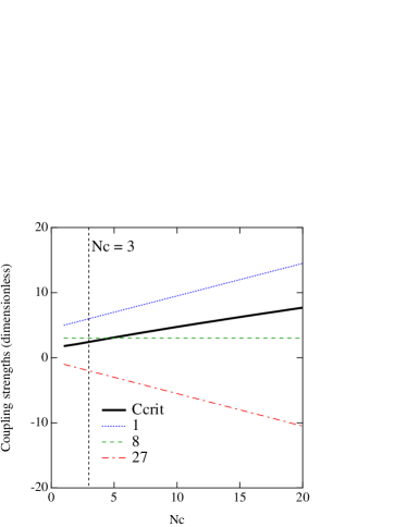
Figure 1: $N_{c}$ dependence of the coupling strengths $C_{\alpha}$ with $\alpha=\mbox{\rm``$\bm{1}$''}$, “$\bm{8}$”, and “$\bm{27}$” (the dotted, dashed, and dash-dotted lines, respectively) together with the critical coupling strength (solid line). The vertical dashed line represents $N_{c}=3$.

As we have noted in Eq. (17), the off-diagonal couplings of the meson-baryon interaction in the isospin basis vanish in the large $N_{c}$ limit. This means that, even with $SU(3)$ breaking, the scattering in the isospin basis behaves as a single-channel problem at sufficiently large $N_{c}$. The coupling strength of $\bar{K}N$ channel in the large $N_{c}$ limit is the same as the one of the singlet channel in the $SU(3)$ basis. Therefore, by following the same argument as the $SU(3)$ symmetric case, we conclude that there is one bound state in the $\bar{K}N$ channel in the large $N_{c}$ limit. It was found in Ref. [49] that the $\bar{K}N$ interaction develops a bound state at $N_{c}=3$, when the transition to other channels are switched off. Thus, as in the $SU(3)$ singlet channel, the $\bar{K}N$ bound state found at $N_{c}=3$ remains in the large $N_{c}$ limit in contrast to the mesonic resonances, while the other states, such as a resonance in $\pi\Sigma$ channel, disappears in the large $N_{c}$ limit.

In this section, we have found that the meson-baryon state remains bound in the large $N_{c}$ limit, both in the $SU(3)$ singlet channel and in the $\bar{K}N$ channel. It is interesting to consider the relation of this result to the kaon bound state approach to the Skyrmion [74, 75]. In this picture based on $1/N_{c}$ expansion, the $\Lambda(1405)$ is described as one bound state of an antikaon and a nucleon. In the chiral unitary approach, the $\Lambda(1405)$ is described as the two poles generated by the attractive interaction in $\bar{K}N$ and $\pi\Sigma$ channels. But taking the large $N_{c}$ limit, only one of them survives as a bound state in the $\bar{K}N$ channel, which may correspond to the bound state found in the Skyrmion approach. This ensures the correct behavior of our amplitude at large $N_{c}$ limit, while at the same time, it also suggests the importance of the $\pi\Sigma$ interaction which is the subleading effect of the $1/N_{c}$ expansion, when one consider the physical system with $N_{c}=3$.

4.2 Other $N_{c}$ extensions

Thus far we have used the standard large $N_{c}$ extension for the baryon representations given in Eq. (13). The merit of this generalization is that spin, isospin and strangeness of the baryon are the same as those at $N_{c}=3$, while the baryon has different charge and hypercharge from those at $N_{c}=3$. It is known that there are two other extensions of the baryon flavor in arbitrary $N_{c}$ [73]:

$$[p,q]\to \left[p+\frac{N_{c}-3}{3},q+\frac{N_{c}-3}{3}\right],$$ (21)

$$[p,q]\to \left[p+N_{c}-3,q\right].$$ (22)

These extensions have some advantages, but the baryons constructed in these ways have unphysical strangeness and spin (see Ref. [88] for detail). With these extensions, the general expressions of the coupling strengths of the WT term are given in Table 1. It can be seen that the strengths of the exotic channels $[p+1,q+1]$, $[p+2,q-1]$ and $[p-1,q+2]$ have negative or constant dependence on $N_{c}$. In the context of Refs. [39, 40], we confirm that the nonexistence of the attractive interaction in exotic channel in any generalizations of the flavor representations.

Table 1: General expressions of the coupling strengths $C_{\mbox{\rm``$\alpha$''},\mbox{\rm``$T$''}}$ for the baryon representation $T=[p,q]$ with three different $N_{c}$ extensions, Eqs. (13), (21) and (22).

$\alpha$	(13)	(21)	(22)
$[p+1,q+1]$	$\frac{3-N_{c}}{2}-p-q$	$\frac{6-2N_{c}}{3}-p-q$	$3-N_{c}-p-q$
$[p+2,q-1]$	$1-p$	$\frac{6-N_{c}}{3}-p$	$4-N_{c}+p$
$[p-1,q+2]$	$\frac{5-N_{c}}{2}-q$	$\frac{6-N_{c}}{3}-q$	$1-q$
$[p,q]$	3	3	3
$[p,q]$	3	3	3
$[p+1,q-2]$	$\frac{3+N_{c}}{2}+q$	$\frac{6+N_{c}}{3}+q$	$3+q$
$[p-2,q+1]$	$3+p$	$\frac{6+N_{c}}{3}+p$	$N_{c}+p$
$[p-1,q-1]$	$\frac{5+N_{c}}{2}+p+q$	$\frac{6+2N_{c}}{3}+p+q$	$1+N_{c}+p+q$

Turning back to the $S=-1$ and $I=0$ scattering, the relevant channels are $\mbox{\rm``$\alpha$''}=\mbox{\rm``$\bm{1}$''}$, “$\bm{8}$”, and “$\bm{27}$” with $\mbox{\rm``$T$''}=\mbox{\rm``$\bm{8}$''}$. The coupling strengths of these channels are given in Table 2. As seen in the table, the coefficients of the linear $N_{c}$ dependence for the “$\bm{1}$” channel in nonstandard extensions (21) and (22) are $2/3$ and $1$, which are larger than that in the standard extension $1/2$. This means that the singlet bound state exists in all cases. Thus, the qualitative conclusion of the previous subsection remains unchanged when we adopt different methods of the extension of the flavor representations.

Table 2: Coupling strengths relevant for $S=-1$ and $I=0$ meson-baryon scattering with $\mbox{\rm``$T$''}=\mbox{\rm``$\bm{8}$''}$.

“$\alpha$”	(13)	(21)	(22)
“$\bm{1}$”	$\frac{9}{2}+\frac{N_{c}}{2}$	$4+\frac{2N_{c}}{3}$	$3+N_{c}$
“$\bm{8}$”	3	3	3
“$\bm{27}$”	$-\frac{1}{2}-\frac{N_{c}}{2}$	$-\frac{2N_{c}}{3}$	$1-N_{c}$

5 Structures of resonances and comparison with quark picture

In this section we investigate the structure of the resonances obtained in the present formulation with $SU(3)$ breaking by comparing the quark picture of the resonances. The $SU(3)$ breaking effects are implemented in the masses of the pseudoscalar mesons and baryons, which are fitted by the observed masses at $N_{c}=3$. The present model successfully reproduces phenomenological properties of the $\Lambda(1405)$ and $\Lambda(1670)$ very well at $N_{c}=3$. Exploiting the present description of the resonances, we investigate the structure of the resonances. For this purpose, first we show the $N_{c}$ behaviors of the pole positions (mass and width) and the couplings to various channels, and then we interpret the $N_{c}$ behaviors in terms of the inner structure of the resonances by comparing with those expected by the quark picture.

We will not take values of $N_{c}$ very far from $N_{c}=3$ for the following reason. The resonances described by the present formulation can have some admixture of genuine preexisting $qqq$ components for $N_{c}=3$. These components certainly have different $N_{c}$ behaviors than the dynamical molecule, but we do not consider the $N_{c}$ dependence of such component. Hence, for very large $N_{c}$ these admixture could be different from what the resonances have intrinsically. For instance, even if a very small component of the genuine quark state is present at $N_{c}=3$, the genuine quark may show up for sufficiently large $N_{c}$ since the quark states survive in the large $N_{c}$ limit. Thus, in order to study the quark structure of “physical” resonances, we vary $N_{c}$ from 3 to 12 in the analysis.

5.1 $N_{c}$ behaviors of pole positions and coupling strengths

We calculate masses and widths of the resonances in the scattering amplitude given in Eq. (4) by looking for the poles of the amplitude in the complex energy plane numerically. We use the $N_{c}$ dependence of the parameters in this model as already given in Sec. 3. With the $SU(3)$ breaking, the scattering amplitude is calculated in coupled channels and each channel has a different threshold. If the poles appear above the lowest threshold, the pole positions are expressed by complex number and the poles represent resonances with finite widths. As we have discussed in Sec. 2, the $\Lambda(1405)$ is described by two poles in this approach. In addition, this model reproduces the $\Lambda(1670)$ resonance at the same time. Thus, at $N_{c}=3$ we have three poles in the complex energy plane.

Calculating the pole positions of the $s$-wave scattering amplitude with $I=0$ and $S=-1$ as functions of $N_{c}$, we obtain the $N_{c}$ behavior of the pole position. In Fig. 2 we show the positions of three poles; two of them appear in energies of the $\Lambda(1405)$ (upper panels) and the other shows up in energies of the $\Lambda(1670)$ (lower panels). The horizontal axis in Fig. 2 represents the excitation (or binding) energy which is the energy of the resonance measured by the threshold of the relevant channel for the resonance. We take the $\bar{K}N$ channel for the $\Lambda(1405)$ and the $K\Xi$ channel for the $\Lambda(1670)$ as the threshold. Consequently the excitation energies are expressed by $\text{Re}(W_{R})-M_{N}-m_{K}$ for the $\Lambda(1405)$ poles and $\text{Re}(W_{R})-M_{\Xi}-m_{K}$ for the $\Lambda(1670)$. The vertical axis expresses the imaginary part of the pole position. We also show the results for the three different regularization methods of the $G$ function discussed in Sec. 3.3. In the left panels, the results obtained with the dimensional regularization are shown, while in the right panels the results with the scaling cutoff (square points) and the unscaling cutoff (triangles) are presented. The symbols in the lines are placed in steps for $N_{c}$ of $1$ unit from 3 to 12. The discontinuity for the two $\Lambda(1405)$ poles at $\text{Re}(W_{R})-M_{N}-m_{K}=0$ is due to the threshold effect. When the pole crosses the $\bar{K}N$ threshold, the width suddenly increases because the important $\bar{K}N$ decay channel suddenly opens. As another threshold effect, it happens that two mathematical poles close each other are obtained around the threshold with a model parameter set. This is known as “shadow poles” consisting in the presence of two nearby poles associated to the same resonance if the pole is very close to a threshold. It is a consequence of unitarity (see Ref. [89] for further details).

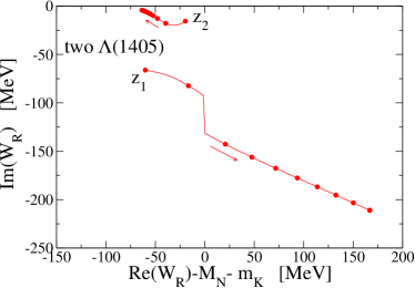
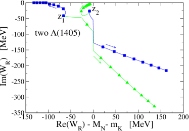
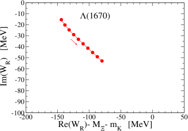
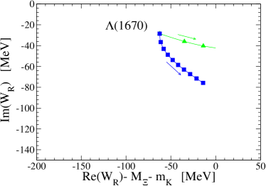
Figure 2: Pole positions of the $s$-wave meson-baryon scattering amplitudes with $I=0$ and $S=-1$ as a function of $N_{c}$ for the three regularization methods discussed in the text. The horizontal axis denotes the real part of the pole position measured by the thresholds of the $\bar{K}N$ channel for the $\Lambda(1405)$ and the $K\Xi$ channel for the $\Lambda(1670)$, and the vertical axis expresses the imaginary part of the pole position. The value of $N_{c}$ varies from 3 to 12 as indicated by arrows. The two upper panels correspond to the two $\Lambda(1405)$ and the lower panel to the $\Lambda(1670)$. The calculation for the plots in the left side, (a) and (c), is done with the dimensional regularization method. The calculation for the plots in the right hand side, (b) and (d), is performed with the cutoff method. The lines with the squares in the right panels is for the scaling cut-off, $q_{\text{max}}\sim{\cal O}(\sqrt{N_{c}})$, while the lines with the triangles is for the unscaling cut-off $q_{\text{max}}\sim{\cal O}(1)$.

Regarding the two $\Lambda(1405)$ poles, one of them approaches the real axis with reducing its width as $N_{c}$ increases. The other $\Lambda(1405)$ pole moves to higher energy region and the imaginary part increases with $N_{c}$. Namely, one $\Lambda(1405)$ resonance tends to become a bound state, while the other tends to dissipate by moving away from the physical axis. For the $\Lambda(1670)$ pole, both the mass and width increase with $N_{c}$, which indicates the tendency of dissipation. These qualitative findings are independent of the choice of the regularization scheme. It is worth mentioning that there is a difference among the choices of the regularization methods: in the dimensional regularization and unscaling cutoff cases, the pole having higher mass at $N_{c}=3$ ($z_{2}$) goes to the bound state as $N_{c}$ increases and the lower pole dissipates, while in the scaling cutoff, the behavior is the other way around. In fact, it is very sensitive to the value of the meson decay constant which pole goes to the bound state in larger $N_{c}$. For instance, if we use a bit larger decay constant like $f(N_{c}=3)=1.2\times 92.4\text{ MeV}$ than the original $f(N_{c}=3)=1.123\times 92.4\text{ MeV}$, the three schemes provide the same behavior, in the sense that the higher pole goes to the bound state. However it is not relevant physically which pole goes to the bound state, but it is important what properties the pole going to the bound state has. As will become clear when we evaluate the flavor components of the poles, the properties of the poles are not dependent on the choice of the regularization schemes. This means that they manifest the qualitative important behavior that one resonance tends to become a bound state while the other one tends to dissipate by moving away from the physical axis.

In order to illustrate further the properties of the dynamically generated resonances, it is very interesting to evaluate the $SU(3)$ contents of the poles as functions of $N_{c}$. This also makes clear connection with the large $N_{c}$ analysis in Sec. 4.1. As explained in Sec. 2, the $SU(3)$ contents of the poles are calculated by the residues of the scattering amplitudes at the pole positions. The coupling constants in the $SU(3)$ basis are obtained in Eq. (12) by the unitary transformation from the isospin basis. In Fig. 3, we show the $N_{c}$ dependence of the coupling ratio, $g_{\alpha}/g_{1}$, for the channel $\alpha$ in absolute value. The calculations are performed using the dimensional regularization method. In order from the top, the panels represent the lower mass $\Lambda(1405)$ (at $N_{c}=3$), the higher mass $\Lambda(1405)$ and the $\Lambda(1670)$ respectively. In the central panel we can see that the the higher pole of the $\Lambda(1405)$ becomes dominantly the singlet flavor-$SU(3)$ state as $N_{c}$ increases, while the lower $\Lambda(1405)$ pole, which goes to infinite width, becomes essentially $\bm{8}$ and the $\Lambda(1670)$ one becomes essentially $\bm{8}^{\prime}$. This is consistent with what we have found in the large $N_{c}$ limit.

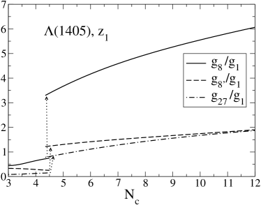
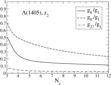
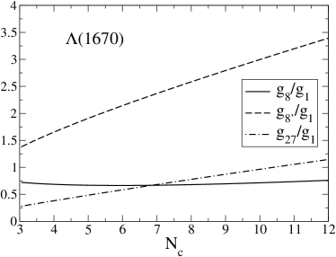
Figure 3: Couplings of the three poles in the $SU(3)$ basis divided by the singlet channel, $g_{\alpha}/g_{1}$. The calculation is done with the dimensional regularization method. The two upper panels correspond to the two $\Lambda(1405)$ and the lower panel to the $\Lambda(1670)$.

In Fig. 4 we also show the couplings of the three poles in the isospin basis by taking their ratios of the coupling to the $\bar{K}N$ channel for reference, $|g_{i}|/|g_{\bar{K}N}|$. We can see in the upper panel that the lower $\Lambda(1405)$ pole, which becomes essentially octet for larger $N_{c}$, couples dominantly to the $\pi\Sigma$ state. On the contrary, the higher $\Lambda(1405)$ pole, shown in the central panel, couples dominantly to $\bar{K}N$. The lower panel in Fig. 4 shows that the strongest coupling of the $\Lambda(1670)$ to the $K\Xi$ state gets weaker as $N_{c}$ increases and the coupling to the $\eta\Lambda$ channel becomes stronger.

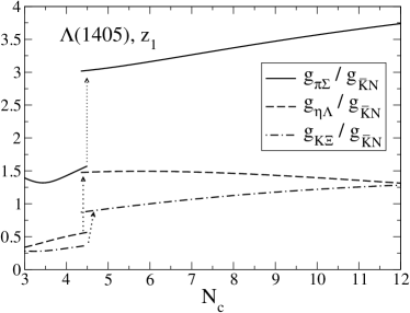
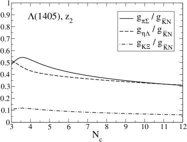
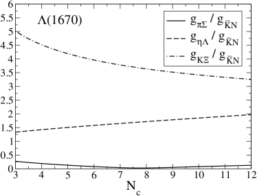
Figure 4: Couplings of the three poles in the isospin basis divided by the $\bar{K}N$ channel, $g_{i}/g_{\bar{K}N}$. The calculation is done with the dimensional regularization method. The two upper panels correspond to the two $\Lambda(1405)$ and the lower panel to the $\Lambda(1670)$.

These analyses of the coupling strengths indicate that the dominant component of the resonances associated with the pole becoming bound state is flavor singlet ($\bar{K}N$) in the $SU(3)$ (isospin) basis, whereas such component in the dissipating resonance becomes less important.

It is interesting to evaluate the coupling strengths of the two $\Lambda(1405)$ poles with the scaling cutoff method because, in this case, as we have already seen above (see Fig. 2 and the squares in Fig. 2), the movement of the poles is different from that obtained in the dimensional regularization scheme, that is, the lower mass pole is the one becoming the bound state.

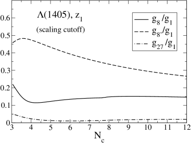
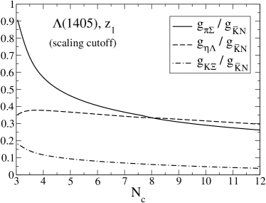
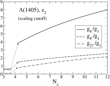
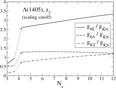
Figure 5: Couplings of the $\Lambda(1405)$ poles using the scaling cutoff regularization method.

Evaluating the residues in the same way, we see in Fig. 5 that the lower mass pole ($z_{1}$) is dominated by the singlet ($\bar{K}N$) in the scaling cutoff scheme. Therefore, the dominance of the flavor singlet and $\bar{K}N$ components for the would-be-bound-state is independent of the choice of the regularization schemes and the original position of the poles at $N_{c}=3$. This result leads us to conjecture that the pole showing the tendency to become a bound state is smoothly connected to the bound state found in the idealized large $N_{c}$ limit.

5.2 The $N_{c}$ scaling of the resonance parameters

In this section, we investigate the internal structure of the resonances based on the findings obtained by the above analyses. As explained in the introduction, the study of the $N_{c}$ dependence of the resonance parameters, such as mass $M_{R}$, excitation energy $\Delta E\equiv M_{R}-M-m$ and width $\Gamma_{R}$, can provide relevant information on the nature of the resonances by comparing to the quark picture. QCD establishes particular $N_{c}$ behaviors for ordinary $qqq$ baryons as

$$M_{R}\sim{\cal O}(N_{c}),\quad\Delta E\sim{\cal O}(1),\quad\Gamma_{R}\sim{\cal O}(1).$$ (23)

Therefore, any deviation of our calculation from these general counting rules for $qqq$ baryons suggests the dynamical origin of the resonances under consideration.

Let us study first the $N_{c}$ dependence of the mass of the resonance. The mass of the resonance is obtained by the real part of the pole position. In Fig. 6, we show the masses of the resonances normalized by the values at $N_{c}=3$, $M_{R}(N_{c})/M_{R}(3)$, for the three poles obtained with the dimensional regularization method. This figure shows that an almost linear $N_{c}$ dependence is obtained for each state. This looks consistent with Eq. (23), but it may not directly lead to the conclusion that these resonances are $qqq$ dominant states. For instance, the $N_{c}$ scaling of a meson-baryon molecule state would be $M_{MB}\sim M_{B}+m\sim{\cal O}(N_{c})$ where we used the scaling of ground state mesons and baryons, and assumed that the binding (excited) energy of the molecule is small compared to $M_{MB}$. If this is the case, the meson-baryon molecule state cannot be distinguished from the $qqq$ state, by looking at the $N_{c}$ behavior of the masses. In this respect, the $N_{c}$ scaling of the mass is not very useful to disentangle the $qqq$ state from the dynamical content.

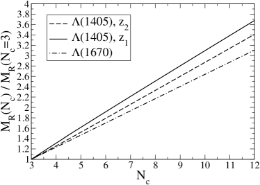
Figure 6: Resonance masses as functions of $N_{c}$ for the three poles normalized to the value at $N_{c}=3$. The calculation is done with the dimensional regularization method.

Next we consider the $N_{c}$ scaling of the excitation energy. In Fig. 7 we plot the excitation (or binding) energies $\Delta E\equiv M_{R}-M_{B}-m$ of the three poles as functions of $N_{c}$. We have normalized $\Delta E$ to the value at $N_{c}=3$ for each particular pole.

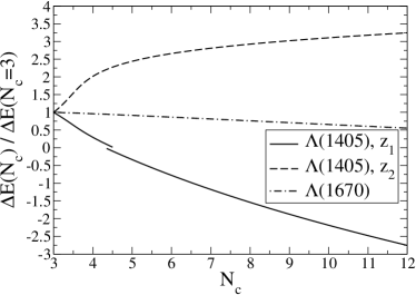
Figure 7: Resonance excitation energy, ($\Delta E\equiv M_{R}-M_{B}-m$), as a function of $N_{c}$ for the three different poles normalized to the value at $N_{c}=3$. The calculation is done for the dimensional regularization method.

QCD predicts for $qqq$ baryons that $\Delta E\sim{\cal O}(1)$ [64, 76, 77]. We see in Fig. 7 that our results do not manifest the constant behavior. For all the poles $\Delta E$ increases in their magnitude as $N_{c}$ increases. Since $\Delta E$ is much smaller than $M_{R}$ and $M_{B}+m$, it barely modifies the linear behavior of $M_{R}$ in Fig. 6. One should keep in mind that these resonances are generated within a coupled channel model and hence several meson-baryon states ($\bar{K}N$, $\pi\Sigma$, $\eta\Lambda$ and $K\Xi$) contribute to their composition. Therefore, the simplified interpretation of the binding (excitation) energy should be taken with care. Hence, the study of the $N_{c}$ dependence of $\Delta E$ should also be considered as indicative but not conclusive.

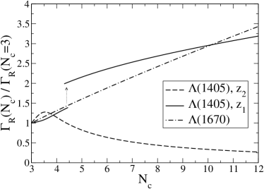
Figure 8: $N_{c}$ behavior of the widths of the two-$\Lambda(1405)$ and the $\Lambda(1670)$ resonance. The calculation is done for the dimensional regularization method.

Much more illustrative and conclusive statements for the understanding of the nature of these resonances can be obtained by studying the $N_{c}$ scaling of the resonance width, $\Gamma_{R}$. The resonance width is given by twice the imaginary part of the pole position. In Fig. 8 we show $\Gamma_{R}$ normalized to the value at $N_{c}=3$ for the dimensional regularization method. The general QCD counting rule for $qqq$ baryons predicts ${\cal O}(1)$ behavior for the width of an excited baryon. Our results are clearly different from this constant behavior. The width of the higher $\Lambda(1405)$ pole (dashed line), which tends to become a singlet state, goes to zero as $N_{c}$ increases. This is again essentially a consequence of the non-trivial $N_{c}$ dependence of the meson-baryon interaction steming from the $N_{c}$ dependence of the $SU(3)$ representation for baryons. The widths of the other $\Lambda(1405)$ and the $\Lambda(1670)$ poles increase with $N_{c}$. In all the cases the widths of the resonances do not follow the constant behavior expected from the general counting rules for the widths of $qqq$ states. We have checked that the results with the other regularization methods (cutoff), not shown in the figure, are similar and hence our results are independent of the choice of the renormalization procedure and its $N_{c}$ dependence.

6 Conclusions

We have studied the $N_{c}$ behavior of the baryon resonances and meson-baryon scatterings with $S=-1$ and $I=0$ from the viewpoint of the chiral unitary approach. Introducing $N_{c}$ dependence of the model parameters, we have analyzed two different situations; meson-baryon scattering in the large $N_{c}$ limit, and the $N_{c}$ behavior of the $\Lambda(1405)$ and $\Lambda(1670)$ resonances not very far from $N_{c}=3$. We have discussed important and nontrivial $N_{c}$ dependence in the Weinberg-Tomozawa interaction, which leads to an ${{\cal O}(1)}$ attraction in the large $N_{c}$ limit for the flavor singlet channels in the $SU(3)$ bases. The attractive interaction in this channel is strong enough to create a bound state, unlike the states associated to the other representations. The existence of this bound state does not depend on the framework of the large $N_{c}$ extension of baryon representations. We have obtained the coupling strengths in the isospin basis through the Clebsch-Gordan coefficients with $N_{c}$ dependence. It is found that the transition between isospin channels vanishes in the large $N_{c}$ limit, and the diagonal $\bar{K}N$ channel manifests an ${{\cal O}(1)}$ attraction, which is again sufficiently strong to generate a bound state in the large $N_{c}$ limit.

In order to investigate the properties of physical resonances, we have explicitly broken flavor $SU(3)$ symmetry by using the physical pseudoscalar and baryon masses. On top of the trivial $N_{c}$ dependences of hadron masses and decay constants, we have included the $N_{c}$ dependences of the WT interaction and the cutoff scale in different regularization methods. The positions and residues of the poles associated to the $\Lambda(1405)$ and the $\Lambda(1670)$ resonances have been studied as functions of $N_{c}$. It is found that one of the two $\Lambda(1405)$ poles tends to become a bound state, and the other $\Lambda(1405)$ and the $\Lambda(1670)$ poles are dissolving into the scattering states. The coupling strengths tell us that the pole becoming the bound state is essentially dominated by the flavor singlet and isospin $\bar{K}N$ components, while the dissolving states are made of other components. This observation indicates that the pole with decreasing width will eventually become the bound state found in the large $N_{c}$ limit. These results are independent of the renormalization procedure and its $N_{c}$ dependence.

We have also evaluated the $N_{c}$ dependence of the mass, excitation energy and width of the $\Lambda(1405)$ and the $\Lambda(1670)$ resonances. The results for the width are at odds with the general QCD counting rules for $qqq$ states. This means that the nature of these resonances are definitely not dominated by the $qqq$ component. These findings reinforce the meson-baryon “molecule” nature of the $\Lambda(1405)$ and the $\Lambda(1670)$ resonances within the chiral unitary approach.

The technique used and the results obtained regarding the $N_{c}$ behavior of these baryonic resonances represent a step forward in the understanding of the connection with the underlying QCD degrees of freedom and the method can be apllied to study other baryonic resonances.

References

- [1] R. L. Jaffe, Phys. Rev. D 15 (1977) 267.
- [2] M. G. Alford and R. L. Jaffe, Nucl. Phys. B 578 (2000) 367.
- [3] T. Kunihiro, S. Muroya, A. Nakamura, C. Nonaka, M. Sekiguchi and H. Wada [SCALAR Collaboration], Phys. Rev. D 70 (2004) 034504.
- [4] C. McNeile, arXiv:0710.0985 [hep-lat].
- [5] A. Dobado and J. R. Pelaez, Phys. Rev. D 56 (1997) 3057.
- [6] J. A. Oller and E. Oset, Nucl. Phys. A 620 (1997) 438, Erratum-ibid. A 652 (1999) 407.
- [7] J. A. Oller, E. Oset and J. R. Pelaez, Phys. Rev. D 59 (1999) 074001, Erratum-ibid. D 60 (1999) 099906 , D75 (2007) 099903.
- [8] J. A. Oller and E. Oset, Phys. Rev. D 60 (1999) 074023.
- [9] R. H. Dalitz and S. F. Tuan, Annals Phys. 10 (1960) 307.
- [10] R. H. Dalitz, T. C. Wong and G. Rajasekaran, Phys. Rev. 153 (1967) 1617.
- [11] N. Isgur and G. Karl, Phys. Rev. D 18 (1978) 4187.
- [12] W. Melnitchouk et al., Phys. Rev. D 67 (2003) 114506.
- [13] Y. Nemoto, N. Nakajima, H. Matsufuru and H. Suganuma, Phys. Rev. D 68 (2003) 094505.
- [14] F. X. Lee and C. Bennhold, Nucl. Phys. A 754 (2005) 248.
- [15] N. Ishii, T. Doi, M. Oka and H. Suganuma, Prog. Theor. Phys. Suppl. 168 (2007) 598.
- [16] N. Kaiser, P. B. Siegel, and W. Weise, Nucl. Phys. A 594 (1995) 325.
- [17] E. Oset and A. Ramos, Nucl. Phys. A 635 (1998) 99.
- [18] J. A. Oller and U. G. Meissner, Phys. Lett. B 500 (2001) 263.
- [19] M. F. M. Lutz and E. E. Kolomeitsev, Nucl. Phys. A 700 (2002) 193.
- [20] T. Hyodo, D. Jido and L. Roca, Phys. Rev. D 77 (2008) 056010.
- [21] S. Weinberg, Physica A 96 (1979) 327.
- [22] J. Gasser and H. Leutwyler, Annals Phys. 158 (1984) 142.
- [23] J. Gasser and H. Leutwyler, Nucl. Phys. B 250 (1985) 465.
- [24] N. Kaiser, Eur. Phys. J. A 3 (1998) 307.
- [25] V. E. Markushin, Eur. Phys. J. A 8 (2000) 389.
- [26] M. F. M. Lutz and E. E. Kolomeitsev, Nucl. Phys. A 730 (2004) 392.
- [27] L. Roca, E. Oset and J. Singh, Phys. Rev. D 72 (2005) 014002.
- [28] N. Kaiser, P. B. Siegel and W. Weise, Phys. Lett. B 362 (1995) 23.
- [29] N. Kaiser, T. Waas and W. Weise, Nucl. Phys. A 612 (1997) 297.
- [30] B. Krippa, Phys. Rev. C 58 (1998) 1333.
- [31] J. Nieves and E. Ruiz Arriola, Phys. Lett. B 455 (1999) 30.
- [32] J. C. Nacher, A. Parreno, E. Oset, A. Ramos, A. Hosaka and M. Oka, Nucl. Phys. A 678 (2000) 187.
- [33] E. Oset, A. Ramos and C. Bennhold, Phys. Lett. B 527 (2002) 99, Erratum-ibid. B 530 (2002) 260.
- [34] T. Inoue, E. Oset and M. J. Vicente Vacas, Phys. Rev. C 65 (2002) 035204.
- [35] D. Jido, A. Hosaka, J. C. Nacher, E. Oset and A. Ramos, Phys. Rev. C 66 (2002) 025203
- [36] D. Jido, E. Oset and A. Ramos, Phys. Rev. C 66 (2002) 055203
- [37] S. Weinberg, Phys. Rev. Lett. 17 (1966) 616.
- [38] Y. Tomozawa, Nuovo Cim. 46A (1966) 707.
- [39] T. Hyodo, D. Jido, and A. Hosaka, Phys. Rev. Lett. 97 (2006) 192002.
- [40] T. Hyodo, D. Jido, and A. Hosaka, Phys. Rev. D 75 (2007) 034002.
- [41] P. J. Fink, G. He, R. H. Landau and J. W. Schnick, Phys. Rev. C 41 (1990) 2720.
- [42] D. Jido, J. A. Oller, E. Oset, A. Ramos, and U. G. Meissner, Nucl. Phys. A 725 (2003) 181.
- [43] T. Hyodo, S. I. Nam, D. Jido and A. Hosaka, Phys. Rev. C 68 (2003) 018201.
- [44] T. Hyodo, S. I. Nam, D. Jido, and A. Hosaka, Prog. Theor. Phys. 112 (2004) 73.
- [45] B. Borasoy, R. Nissler, and W. Weise, Eur. Phys. J. A 25 (2005) 79.
- [46] J. A. Oller, J. Prades, and M. Verbeni, Phys. Rev. Lett. 95 (2005) 172502.
- [47] J. A. Oller, Eur. Phys. J. A 28 (2006) 63.
- [48] B. Borasoy, U. G. Meissner, and R. Nissler, Phys. Rev. C 74 (2006) 055201.
- [49] T. Hyodo and W. Weise, Phys. Rev. C 77 (2008) 03524.
- [50] S. Prakhov et al. [Crystall Ball Collaboration], Phys. Rev. C 70 (2004) 034605.
- [51] V. K. Magas, E. Oset, and A. Ramos, Phys. Rev. Lett. 95 (2005) 052301.
- [52] I. Zychor et al., Phys. Lett. B 660 (2008) 167.
- [53] L. S. Geng and E. Oset, arXiv:0707.3343 [hep-ph].
- [54] T. Hyodo, A. Hosaka, E. Oset, A. Ramos, and M. J. Vicente Vacas, Phys. Rev. C 68 (2003) 065203.
- [55] L. S. Geng, E. Oset and M. Doring, Eur. Phys. J. A 32 (2007) 201.
- [56] T. Hyodo, A. Hosaka, M. J. Vicente Vacas, and E. Oset, Phys. Lett. B 593 (2004) 75.
- [57] R. J. Hemingway, Nucl. Phys. B 253 (1985) 742.
- [58] R. H. Dalitz and A. Deloff, J. Phys. G 17 (1991) 289.
- [59] Y. Akaishi and T. Yamazaki, Phys. Rev. C 65 (2002) 044005.
- [60] T. Yamazaki and Y. Akaishi, Phys. Rev. C 76 (2007) 045201.
- [61] A. Doté, T. Hyodo and W. Weise, arXiv:0802.0238 [nucl-th], Nucl. Phys. A, in press.
- [62] D. B. Kaplan and A. E. Nelson, Phys. Lett. B 175 (1986) 57.
- [63] G. ’t Hooft, Nucl. Phys. B 72 (1974) 461.
- [64] E. Witten, Nucl. Phys. B 160 (1979) 57.
- [65] E. Witten, Annals Phys. 128 (1980) 363.
- [66] J. R. Pelaez, Phys. Rev. Lett. 92 (2004) 102001.
- [67] J. R. Pelaez and G. Rios, Phys. Rev. Lett. 97 (2006) 242002.
- [68] J. R. Pelaez, Mod. Phys. Lett. A 19 (2004) 2879.
- [69] L. S. Geng, E. Oset, J. R. Pelaez ad L. Roca, submitted to Phys. Lett. B , preprint IFIC-07-1028
- [70] R. L. Jaffe, Prog. Theor. Phys. Suppl. 168 (2007) 127.
- [71] G. Karl, J. Patera, and S. Perantonis, Phys. Lett. B 172 (1986) 49.
- [72] Z. Dulinski and M. Praszalowicz, Acta Phys. Polon. B 18 (1988) 1157.
- [73] Z. Dulinski, Acta Phys. Polon. B 19 (1988) 891.
- [74] C. G. Callan and I. R. Klebanov, Nucl. Phys. B 262 (1985) 365.
- [75] N. Itzhaki, I. R. Klebanov, P. Ouyang, and L. Rastelli, Nucl. Phys. B 684 (2004) 264.
- [76] J. L. Goity, Phys. Atom. Nucl. 68 (2005) 624.
- [77] T. D. Cohen, D. C. Dakin, A. Nellore, and R. F. Lebed, Phys. Rev. D 69 (2004) 056001.
- [78] C. Garcia-Recio, J. Nieves and L. L. Salcedo, Phys. Rev. D 74 (2006) 036004.
- [79] V. Bernard, N. Kaiser and U. G. Meissner, Int. J. Mod. Phys. E 4 (1995) 193.
- [80] J. J. de Swart, Rev. Mod. Phys. 35 (1963) 916.
- [81] P. S. J. McNamee and F. Chilton, Rev. Mod. Phys. 36 (1964) 1005.
- [82] E. E. Jenkins and R. F. Lebed, Phys. Rev. D 52 (1995) 282
- [83] R. F. Dashen and A. V. Manohar, Phys. Lett. B 315 (1993) 425.
- [84] R. F. Dashen and A. V. Manohar, Phys. Lett. B 315 (1993) 438.
- [85] T. D. Cohen and R. F. Lebed, Phys. Rev. D 70 (2004) 096015.
- [86] T. Hyodo, D. Jido and A. Hosaka, Prog. Theor. Phys. Suppl. 168 (2007) 32.
- [87] T. Hyodo, D. Jido and A. Hosaka, arXiv:0803.2550 [nucl-th].
- [88] K. Piesciuk and M. Praszalowicz, Prog. Theor. Phys. Suppl. 168 (2007) 70.
- [89] R. J. Eden and J. R. Taylor, Phys. Rev. 133, B1575 - B1580 (1964); M. Ross, Phys. Rev. Lett. 11, 450 - 453 (1963).