Application of Gaussian expansion method to nuclear mean-field calculations with deformation

We extensively develop a method of implementing mean-field calculations for deformed nuclei, using the Gaussian expansion method (GEM). This GEM algorithm has the following advantages: (i) it can efficiently describe the energy-dependent asymptotics of the wave functions at large $r$, (ii) it is applicable to various effective interactions including those with finite ranges, and (iii) the basis parameters are insensitive to nuclide, thereby many nuclei in wide mass range can be handled by a single set of bases. Superposing the spherical GEM bases with feasible truncation for the orbital angular momentum of the single-particle bases, we obtain deformed single-particle wave-functions to reasonable precision. We apply the new algorithm to the Hartree-Fock and the Hartree-Fock-Bogolyubov calculations of Mg nuclei with the Gogny interaction, by which neck structure of a deformed neutron halo is suggested for ⁴⁰Mg.

PACS numbers: 21.60.Jz, 21.10.Gv, 21.10.Dr, 27.30.+t

Keywords: Mean-field calculation; Gaussian expansion method; axially-symmetric deformation; finite-range interaction; deformed neutron halo

1 Introduction

As experimental facilities supply fruitful data on nuclei far off the $\beta$-stability, it has been recognized that theoretical approaches to nuclear structure should be renewed in some respects. One of the key ingredients is wave-function asymptotics at large $r$, which sometimes produces neutron (proton) halos in vicinity of the neutron (proton) drip line. It is also important to reinvestigate effective interactions, in connection to the magic numbers that are different from those near the $\beta$-stability line. We developed a method for the spherical mean-field calculations [1, 2] in which the Gaussian expansion method (GEM) [3] was applied. This method seems suitable to studying the shell structure from stable to drip-line nuclei, owing to its several advantages.

A large number of nuclei have quadrupole deformation. The deformation plays a significant role in unstable nuclei as well. For instance, the deformation can be relevant to the disappearance of the $N=20$ magic number on the so-called ‘island of inversion’ [4], whereas there remain arguments for individual nuclei; e.g. spherical description has also been proposed for ³²Mg [5]. It is desired to implement calculations with deformation, reproducing the wave-function asymptotics and handling a wide variety of effective interactions simultaneously.

In this paper we propose a new method for deformed mean-field calculations by applying the GEM. Taking advantage of the flexibility in describing the radial degrees of freedom, we adopt a set of the spherical GEM bases to represent deformed single-particle (s.p.) wave functions, with truncation for the orbital angular momentum $\ell$. The new method is tested in the Hartree-Fock (HF) and the Hartree-Fock-Bogolyubov (HFB) calculations for Mg nuclei with the Gogny interaction, and the results are compared with those in literatures. From the present calculation, an interesting feature is suggested for the drip-line nucleus ⁴⁰Mg.

2 Single-particle bases

In this paper we assume the nuclear mean fields to be axially symmetric and to conserve the parity. The $z$ axis is taken to be the symmetry axis. The method can immediately be extended to general cases with no symmetry assumptions on the one-body fields, apart from an additional constraint on the center-of-mass (c.m.) position.

2.1 GEM bases

We represent the s.p. wave functions by superposing the spherical Gaussian bases, which have the following form:

$$\varphi_{\nu\ell jm}(\mathbf{r}) = R_{\nu\ell j}(r)\,[Y^{(\ell)}(\hat{\mathbf{r}})\chi_{\sigma}]^{(j)}_{m}\,;$$

$$R_{\nu\ell j}(r) = \mathcal{N}_{\nu\ell j}\,r^{\ell}\exp(-\nu r^{2})\,.$$ (1)

Here $Y^{(\ell)}(\hat{\mathbf{r}})$ expresses the spherical harmonics and $\chi_{\sigma}$ the spin wave function. We drop the isospin index without confusion. The range parameter of the Gaussian basis $\nu$ is a complex number in general [6]; $\nu=\nu_{\mathrm{r}}+i\nu_{\mathrm{i}}$ ($\nu_{\mathrm{r}}>0$). Via the imaginary part oscillating behavior of the s.p. wave functions can be expressed efficiently [2]. Formulae for calculating the one- and two-body matrix elements that are required in the HF and the HFB calculations, as well as the constant $\mathcal{N}_{\nu\ell j}$, are given in Refs. [1, 2]. The s.p. wave functions under the axially deformed mean field are represented as

$$\psi_{n\pi m}(\mathbf{r})=\sum_{\nu\ell j}c^{(n)}_{\nu\ell jm}\,\varphi_{\nu\ell jm}(\mathbf{r})\,,$$ (2)

where the subscript $\pi$ on the lhs stands for the parity. The sum of $\ell$ and $j$ on the rhs runs over all possible values satisfying $\pi=(-)^{\ell}$, $j=\ell\pm 1/2$ and $j\geq|m|$, in principle.

In the GEM we usually take $\nu$’s belonging to a geometric progression. In Ref. [2], we found that a certain combination of the real- and complex-range Gaussian bases is suitable for nuclear mean-field calculations. In all the following calculations, we take the basis-set of

$$\nu_{\mathrm{r}}=\nu_{0}\,b^{-2n}\,,\quad\left\{\begin{array}[]{ll}\nu_{\mathrm{i}}=0&(n=0,1,\cdots,5)\\ {\displaystyle\frac{\nu_{\mathrm{i}}}{\nu_{\mathrm{r}}}=\pm\frac{\pi}{2}}&(n=0,1,2)\end{array}\right.\,,$$ (3)

with $\nu_{0}=(2.40\,\mathrm{fm})^{-2}$ and $b=1.25$, irrespective of $(\ell,j)$. Namely, 12 bases are employed for each $(\ell,j)$; 6 bases have real $\nu$ and the other 6 have complex $\nu$. This set is quite similar to Set C in Ref. [2].

2.2 Adaptability to wave functions with various size

An appropriate set of the GEM bases is capable of describing wave functions with various size. This feature is desirable for self-consistent mean-field calculations with deformation, because in deformed nuclei the density distribution depends on the direction, and degree of the deformation is not known in advance. We here show adaptability of the GEM with respect to size of nuclei, by presenting results of the spherical Hartree-Fock (HF) calculations.

Size of spherical nuclei, which is typically represented by the rms radii, depends on the mass number $A$, apart from exotic structure such as neutron halos near the drip line. Many mean-field calculations have been implemented by using the harmonic oscillator (HO) bases, particularly when the effective interaction has finite ranges. In the mean-field calculations with the HO bases, the length parameter of the bases $b_{\omega}=1/\sqrt{M\omega}$ depends on $A$. For stable nuclei, $b_{\omega}$ is almost proportional to $A^{1/6}$, as $\omega\approx 41.2\,A^{-1/3}\,\mathrm{MeV}$, although $b_{\omega}$ is often adjusted for individual nuclides so as to minimize their energy $E$. In contrast, since the GEM basis-set contains Gaussians of various ranges, even a single set can describe many nuclei to good precision. Binding energies and rms matter radii calculated with the Gogny D1S interaction [7] are tabulated in Table 1, for the doubly-magic nuclei ¹⁶O, ²⁴O, ⁴⁰Ca, ⁴⁸Ca, ⁹⁰Zr and ²⁰⁸Pb. The values obtained from the GEM basis-set of Eq. (3) are compared with those from the $A$-dependent HO basis-set. The Coulomb interaction between protons is handled exactly [1], and the c.m. motion is fully removed from the effective Hamiltonian before variation. The influence of the c.m. motion on the rms matter radii is treated in a similar manner [8]. In the calculations using the HO bases, the $b_{\omega}$ parameter of the bases is determined from $\omega=41.2\,A^{-1/3}\,\mathrm{MeV}$, and all the bases up to $N_{\mathrm{osc}}=15$ are included, where $N_{\mathrm{osc}}$ is number of the oscillator quanta. Because of the variational nature of the HF theory, the lower energy indicates the more reliable result for individual nuclei. In this regard, the $A$-independent set of the GEM bases gives no worse, even slightly better results than the $A$-dependent HO basis-set except for ¹⁶O. To show further the adaptability of the GEM basis-set to nuclear size, the calculated density distributions of the six nuclei are illustrated in Fig. 1.

Table 1: Binding energies $-E$ ($\mathrm{MeV}$) and rms matter radii $\sqrt{\langle r^{2}\rangle}$ ($\mathrm{fm}$) of ¹⁶O, ²⁴O, ⁴⁰Ca, ⁴⁸Ca, ⁹⁰Zr and ²⁰⁸Pb in the HF calculations with the D1S interaction. Results of the GEM bases and the HO bases are compared.

Nuclide		HO	GEM
16O	$-E$	$129.638$	$129.520$
	$\sqrt{\langle r^{2}\rangle}$	$2.603$	$2.606$
24O	$-E$	$168.573$	$168.598$
	$\sqrt{\langle r^{2}\rangle}$	$2.998$	$3.014$
40Ca	$-E$	$344.470$	$344.570$
	$\sqrt{\langle r^{2}\rangle}$	$3.370$	$3.370$
48Ca	$-E$	$416.567$	$416.764$
	$\sqrt{\langle r^{2}\rangle}$	$3.514$	$3.513$
90Zr	$-E$	$785.126$	$785.928$
	$\sqrt{\langle r^{2}\rangle}$	$4.238$	$4.235$
208Pb	$-E$	$1638.094$	$1639.047$
	$\sqrt{\langle r^{2}\rangle}$	$5.517$	$5.513$

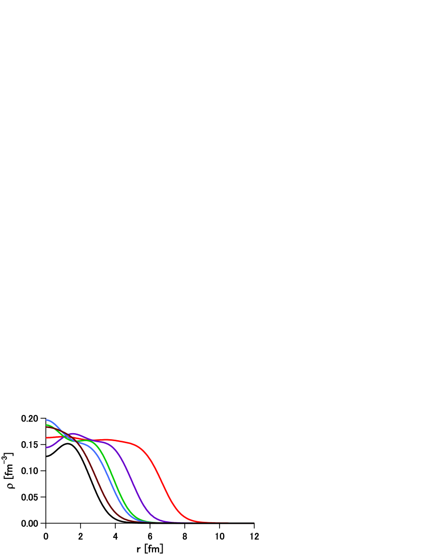
Figure 1: Density distribution of ¹⁶O (black line), ²⁴O (brown line), ⁴⁰Ca (blue line), ⁴⁸Ca (green line), ⁹⁰Zr (purple line) and ²⁰⁸Pb (red line), calculated by the GEM basis-set with the D1S interaction.

In the results of Table 1, we use larger number of bases in the GEM calculation than in the HO calculation. Although one might think that this is not fair comparison, it is not technically easy to increase the number of the HO bases, because of round-off errors. It is rather another advantage of the GEM that we can avoid harmful round-off errors even with a large number of bases. Furthermore, it should be stressed that the GEM basis-set used here is nucleus-independent, demonstrating adaptability to nuclear size. This yields an additional advantage in systematic calculations. In the self-consistent mean-field calculations such as HF and HFB with finite-range interactions, computation of the two-body interaction matrix elements is the most time-consuming part. Since the basis-set of Subsec. 2.1 is applicable to many nuclei, we do not have to repeat computation of the interaction matrix elements once they are stored.

2.3 Test on truncation with respect to $\ell$

As viewed in Eq. (2), there is mixing of $\ell$ and $j$ in the s.p. wave functions under the deformed mean field. In particular, the $\ell$-mixing is relevant to the deformation. The mixing of $j\,(=\ell\pm 1/2)$ is driven by the spin-orbit coupling. In deformed mean-field calculations with the spherical bases, we necessarily truncate the s.p. bases with respect to $\ell$ (and $j$), by restricting the sum over $\ell$ in Eq. (2) as $\ell\leq\ell_{\mathrm{max}}$. It is an unavoidable question how large $\ell_{\mathrm{max}}$ is needed for practical calculations.

To answer this question, we consider an axially symmetric HO potential, giving a s.p. Hamiltonian of

$$\hat{h}=\frac{\mathbf{p}^{2}}{2M}+\frac{M}{2}\left[\omega_{\perp}^{2}(x^{2}+y^{2})+\omega_{z}^{2}z^{2})\right]=\frac{\mathbf{p}^{2}}{2M}+\frac{M}{2}\omega_{0}^{2}\,r^{2}\left[1-\frac{4}{3}\sqrt{\frac{4\pi}{5}}\delta_{\mathrm{def}}\,Y^{(2)}_{0}(\hat{\mathbf{r}})\right]\,,$$ (4)

where $\omega_{0}^{2}=(2\omega_{\perp}^{2}+\omega_{z}^{2})/3$ and $\delta_{\mathrm{def}}=(\omega_{\perp}^{2}-\omega_{z}^{2})/2\omega_{0}^{2}$. The exact eigenvalues of this Hamiltonian are obviously $\varepsilon(n_{\perp}n_{z})=\omega_{\perp}(n_{\perp}+1)+\omega_{z}(n_{z}+\frac{1}{2})$ ($n_{\perp},n_{z}=0,1,\cdots$). On the other hand, we obtain approximate eigenvalues by diagonalizing this Hamiltonian with the spherical GEM bases, by setting a certain value of $\ell_{\mathrm{max}}$. Quality of the $\ell_{\mathrm{max}}$ truncation can be assessed by comparing the approximate solutions to the exact ones.

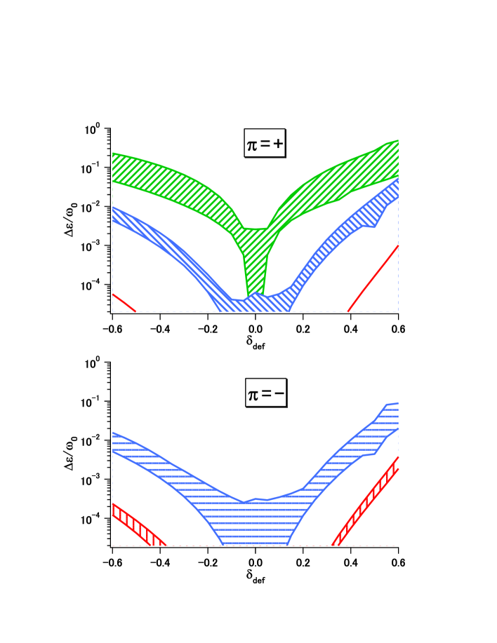
Figure 2: Errors of the GEM solutions in energy eigenvalues of the anisotropic harmonic oscillator of Eq. (4), whose ranges are represented by the hatched areas for each $N_{\mathrm{osc}}$ value. Upper panel: Errors for the $\pi=+$ levels. Red, blue and green areas show bounds of errors for the $N_{\mathrm{osc}}=0$, $2$ and $4$ levels, respectively. Lower panel: Errors for the $\pi=-$ levels. Red and blue areas represent bounds of errors for the $N_{\mathrm{osc}}=1$ and $3$ levels.

In Fig. 2, we plot errors of the energy eigenvalues obtained by the GEM, $\mathit{\Delta}\varepsilon(n_{\perp}n_{z})\equiv\varepsilon_{\mathrm{GEM}}(n_{\perp}n_{z})-\varepsilon_{\mathrm{exact}}(n_{\perp}n_{z})$, as a function of $\delta_{\mathrm{def}}$, taking $\ell_{\mathrm{max}}=7$ with the basis-set of Eq. (3). Although we set $(\omega_{\perp}^{2}\omega_{z})^{1/3}=41.2\,A^{-1/3}\,\mathrm{MeV}$ with $A=24$ at each $\delta_{\mathrm{def}}$, the errors are insensitive to $\omega_{0}$ if we measure $\mathit{\Delta}\varepsilon$ in unit of $\omega_{0}$. We have confirmed that the results presented in Fig. 2 are almost unchanged even for $A=208$. The eigenvalues belonging to equal $N_{\mathrm{osc}}(=n_{\perp}+n_{z})$ have errors of the same orders of magnitude (except at $\delta_{\mathrm{def}}=0$). This is because the levels belonging to equal $N_{\mathrm{osc}}$ significantly mix one another owing to their close energies, while admixture of the $N_{\mathrm{osc}}\pm 2$ levels occurs only perturbatively. We therefore classify the s.p. levels by $N_{\mathrm{osc}}$ and show their errors as a function of $\delta_{\mathrm{def}}$ by the hatched areas, which are edged by the minimum and maximum errors for each $N_{\mathrm{osc}}$.

At $\delta_{\mathrm{def}}=0$ (i.e. $\omega_{\perp}=\omega_{z}$), the energy eigenvalues become $\varepsilon(n_{\perp}n_{z})=\omega_{0}(N_{\mathrm{osc}}+\frac{3}{2})$. The errors at $\delta_{\mathrm{def}}=0$ exclusively come from the choice of the radial parameters in Eq. (3), irrelevant to the $\ell$-mixing. We have much smaller errors at $\delta_{\mathrm{def}}=0$ than those at finite $\delta_{\mathrm{def}}$. Because the radial parts are well described, the errors at $\delta_{\mathrm{def}}\neq 0$ predominantly depend on how well the $\ell$-mixing is taken into account. Irregularities at $\delta_{\mathrm{def}}\geq 0.5$ as well as at $\delta_{\mathrm{def}}=0$ occur due to crossing of the levels that have equal $\pi$ and $m$ quantum numbers.

Whereas it depends on the situation what precision is required in the calculation, we here assume the criterion to be $\mathit{\Delta}\varepsilon\lesssim 0.01\,\omega_{0}$, which corresponds to $\mathit{\Delta}\varepsilon\lesssim 0.1\,\mathrm{MeV}$ for nuclei with $\omega_{0}\sim 10\,\mathrm{MeV}$. With the $\ell_{\mathrm{max}}=7$ truncation, all the $N_{\mathrm{osc}}\leq 3$ levels satisfy this criterion at $-0.5\lesssim\delta_{\mathrm{def}}\lesssim+0.35$. This region of $\delta_{\mathrm{def}}$ covers deformation of most nuclei, as long as their low-energy states are concerned. Since $\mathit{\Delta}\varepsilon$ exceeds $0.01\,\omega_{0}$ even at $\delta_{\mathrm{def}}\approx 0.1$, we cannot expect that the $\ell_{\mathrm{max}}=7$ truncation works well for the $N_{\mathrm{osc}}\geq 4$ levels. It should be noticed that the crossing between the highest level of $N_{\mathrm{osc}}=3$ and the lowest level of $N_{\mathrm{osc}}=5$ takes place at $\delta_{\mathrm{def}}=+0.41$ and $-0.56$. These crossing points are close to the edges of the region where the above criterion is fulfilled. Beyond these $\delta_{\mathrm{def}}$ values some of the $N_{\mathrm{osc}}=5$ levels, for which we need higher $\ell_{\mathrm{max}}$, are occupied before all the $N_{\mathrm{osc}}=3$ levels are, although the crossing levels do not necessarily mix since they may have different quantum numbers $m$. Similar crossing between the $N_{\mathrm{osc}}=4$ and $6$ levels occurs at $\delta_{\mathrm{def}}\approx+0.34$ and $-0.44$. Thus the crossing points between $N_{\mathrm{osc}}$ and $N_{\mathrm{osc}}+2$ levels are not very sensitive to $N_{\mathrm{osc}}$. Although the spin-orbit splitting influences the level crossing points, the current argument will hold in more realistic cases to a good degree, because the spin-orbit splitting is much smaller than $2\omega_{0}$. Thus it will be reasonable to state that we should take $\ell_{\mathrm{max}}\geq N_{\mathrm{osc}}^{F}+4$ in deformed mean-field calculations, where $N_{\mathrm{osc}}^{F}$ is defined to be the highest oscillator quantum number for the s.p. levels under interest. If we take $\ell_{\mathrm{max}}\geq N_{\mathrm{osc}}^{F}+6$, we can expect better precision by about two orders of magnitude; the error on the level corresponding to $N_{\mathrm{osc}}^{F}$ will be $\mathit{\Delta}\varepsilon^{F}\lesssim 10^{-4}\,\omega_{0}$ for low energy states.

While we have discussed errors on the s.p. energies, mean-field calculations are carried out by minimizing the total energy of each nucleus. Because the errors grow for the larger $|\delta_{\mathrm{def}}|$, calculations with the spherical bases tend to yield higher energy for deformed states than for spherical states. We put $N_{\mathrm{osc}}^{F}$ to be the value for the Fermi level, which can be estimated as $N_{\mathrm{osc}}^{F}\approx(3A/2)^{1/3}$ [9]. The number of nucleons occupying the $N_{\mathrm{osc}}^{F}$ levels should be $2(N_{\mathrm{osc}}^{F})^{2}\approx(3\sqrt{2}A)^{2/3}$. Dominated by the errors on the $N_{\mathrm{osc}}^{F}$ levels, error on the total energy due to the $\ell_{\mathrm{max}}$ truncation is estimated to be $\mathit{\Delta}E\approx(3\sqrt{2}A)^{2/3}\,\mathit{\Delta}\varepsilon^{F}$. Inserting $\mathit{\Delta}\varepsilon^{F}\approx 0.01\,\omega_{0}$ and $\omega_{0}\approx 40\,\mathrm{MeV}$, we obtain $\mathit{\Delta}E\approx A^{1/3}\,\mathrm{MeV}$ for well-deformed configurations, while this error is absent in spherical configurations. We should keep this point in mind when comparing energies of a spherical minimum and a deformed one.

3 Implementation of self-consistent mean-field calculations with deformation

We have discussed that the spherical GEM bases shown in Subsec. 2.1 is promising in describing deformed nuclei. We next present how we implement self-consistent HF or HFB calculations using the GEM bases.

One of the advantages of the GEM algorithm in Refs. [1, 2] was that finite-range effective interactions are tractable [8] by computing two-body interaction matrix elements of the interactions, even for the LS and the tensor channels. This advantage is maintained in the deformed cases. While in the spherical cases the number of necessary matrix elements is reduced to great extent due to the symmetry of the one-body fields, we need all the non-vanishing two-body matrix elements in the deformed mean-field calculations. Since we adopt the spherical GEM bases, the matrix elements can straightforwardly be computed according to the formulae shown in Refs. [1, 2]. It costs 4.3 GB of memory or disk to store the matrix elements with $\ell\leq 7$ in double precision. We handle the Coulomb interaction in a similar manner, which needs additional 2.2 GB. Although it is time-consuming task to compute them, those matrix elements are useful for various calculations once we store them; not only for HF and HFB calculations of many nuclei, but also for calculations in the random-phase approximation, as will be discussed elsewhere.

The density-dependent interaction should be renewed at each iteration. This is not a difficult task as long as this part of the interaction has a contact form as in Ref. [8].

Folding the stored matrix elements with given s.p. wave functions, we construct the s.p. Hamiltonian that preserves the $(\pi,m)$ quantum numbers. The s.p. wave functions are then obtained by solving the HF or HFB equation as a generalized eigenvalue problem, for each $(\pi,m)$. Starting from appropriate initial values, we repeat this procedure iteratively until convergence. Alternatively, we can apply the gradient method to obtain the energy minimum by using the s.p. Hamiltonian.

The present algorithm keeps the advantages of the GEM in the spherical mean-field calculations. We here list them again: (i) it is efficient in describing the energy-dependent asymptotics of s.p. wave functions at large $r$, (ii) we can handle various effective interactions, including those having non-locality, and (iii) the basis parameters are insensitive to nuclide, thereby a single-set of bases is applicable to wide mass range of nuclei.

4 Numerical examples for magnesium isotopes

We now apply the present method of the deformed HF and HFB calculations to actual nuclei. We take even-$N$ magnesium isotopes as examples, which contain a well-deformed stable nucleus ²⁴Mg, several nuclei on the island of inversion such as ³²Mg and ³⁴Mg, and ⁴⁰Mg for which the $N=28$ magicity has been predicted to disappear in several calculations. We exactly treat the Coulomb energy [1], and both the one- and two-body terms of the c.m. part are subtracted from the Hamiltonian before variation, unless mentioned explicitly. The GEM bases of Subsec. 2.1 are employed with the $\ell_{\mathrm{max}}=7$ truncation. This fulfills $\ell_{\mathrm{max}}\geq N_{\mathrm{osc}}^{F}+4$ for the ground states of all the Mg nuclei to be presented, since the last neutron occupies an $N_{\mathrm{osc}}=3$ orbit in the neutron-rich Mg nuclei.

4.1 Comparison with previous calculations

We examine how well the present method can describe the deformed Mg nuclei. We first show results of the HF calculation with the D1 parameter-set [10] of the Gogny interaction.

In Ref. [11], an axial HF calculation using the HO bases has been implemented for many Mg isotopes. Although the basis-set consists only of $N_{\mathrm{osc}}\leq 4$, the oscillator length $b_{\omega}$ is optimized except for ³⁶Mg and ³⁸Mg. In Table 2 we compare the present GEM results for the Mg isotopes with those in Ref. [11]. For ^22,24,28Mg, binding energies computed in the antisymmetrized molecular dynamics (AMD) [12] are reported. The AMD is a powerful tool to study structure of light to medium-mass nuclei. In the AMD approach the total wave function is represented by a Slater determinant of Gaussian wave packets of constituent nucleons. While ranges of the Gaussians are taken to be equal for all nucleons in the nucleus, the nucleons have different central positions from one another and the positions are optimized without assuming the axial symmetry. Whereas the AMD has been extended by incorporating the projections and superposing many Slater determinants, we here use the results of its simplest version for comparison, because it is analogous to the HF approximation.

With respect to the spurious c.m. motion, it is popular in the mean-field calculations so far to remove only the one-body term before variation. One of the present GEM results (denoted by GEM₁) are obtained by this prescription. While influence of the spurious c.m. motion can be fully removed in the AMD, only the one-body term is subtracted before variation in the AMD results shown in Table 2. Therefore the GEM₁ values should be compared to the HO and the AMD ones. We additionally present the values in which the two-body term of the c.m. Hamiltonian is also subtracted before variation in the GEM calculation, and denote them by GEM₂.

Table 2: Comparison of the axial HF results for binding energies $-E$ ($\mathrm{MeV}$) and intrinsic mass quadrupole moments $Q_{0}$ ($\mathrm{fm}^{2}$) of the Mg isotopes. The present GEM results are compared with those of the HO bases [11] and the AMD calculation [12]. The one-body c.m. energy is subtracted in GEM₁ as well as in the HO and the AMD results, while the two-body c.m. energy is also removed in GEM₂. The D1 interaction is adopted for all the calculations.

Nuclide		HO	AMD	GEM1	GEM2
22Mg	$-E$	—	$161.26$	$169.03$	$162.44$
	$Q_{0}$	—	—	$100.84$	$104.53$
24Mg	$-E$	$193.90$	$188.33$	$195.73$	$188.74$
	$Q_{0}$	$113.95$	—	$114.39$	$118.11$
26Mg	$-E$	$211.11$	—	$212.99$	$205.29$
	$Q_{0}$	$76.51$	—	$78.20$	$81.09$
28Mg	$-E$	$227.82$	$223.07$	$230.14$	$222.45$
	$Q_{0}$	$101.37$	—	$101.41$	$105.06$
30Mg	$-E$	$237.69$	—	$240.34$	$232.36$
	$Q_{0}$	$76.10$	—	$75.07$	$77.29$
32Mg	$-E$	$245.98$	—	$249.05$	$240.97$
	$Q_{0}$	$34.27$	—	$37.13$	$38.33$
34Mg	$-E$	$249.94$	—	$254.77$	$246.43$
	$Q_{0}$	$111.70$	—	$128.36$	$131.92$
36Mg	$-E$	$253.79$	—	$260.49$	$251.84$
	$Q_{0}$	$146.17$	—	$176.50$	$180.81$
38Mg	$-E$	$251.69$	—	$261.69$	$252.62$
	$Q_{0}$	$168.65$	—	$175.06$	$179.47$

Since the HF approximation holds variational nature, the lower ground-state energy indicates the more reliable result (i.e. the closer to the true minimum). In this respect the present GEM bases give more favorable results than the HO and the AMD bases. The present method gives $7-8\,\mathrm{MeV}$ lower energies than the AMD in ^22,24,28Mg. Compared to the HO calculation in Ref. [11], the energy gain in the present calculation grows as going to the neutron-rich region, $\sim 2\,\mathrm{MeV}$ in ²⁴Mg to $\sim 10\,\mathrm{MeV}$ in ³⁸Mg. It may be due to spatially broad distribution of density in the neutron-rich region, which is well described by the GEM but is hard to be reproduced with the HO bases. It should be noticed that ³⁸Mg is unbound in the result of Ref. [11] because it has higher energy than ³⁶Mg, while it is bound in the present calculation. This exemplifies importance of numerical algorithm that appropriately handles spatial extension of wave functions when investigating the neutron drip line.

The two-body term of the c.m. Hamiltonian affects the energies to sizable amount, as clearly viewed in Table 2. Difference between the GEM₁ and GEM₂ energies slightly grows for increasing $A$.

We next turn to the HFB calculations. We compare the GEM results for ^30-34Mg with those obtained from the HO bases truncated by $N_{\mathrm{osc}}\leq 10$ [13], in Table 3. The D1S parameter-set [7] of the Gogny interaction is adopted, and the c.m. Hamiltonian is fully subtracted before iteration in both calculations. In Ref. [13], the spherical HO bases are used, so that the angular-momentum projection could be carried out afterward. The exchange term of the Coulomb energy is handled in the Slater approximation in Ref. [13].

Table 3: Binding energies $-E$ (MeV) of ^30,32,34Mg in the HFB calculations with the D1S interaction. The GEM results are compared with those of the HO bases in Ref. [13].

Nuclide	HO	GEM	Exp.
30Mg	$239.30~{}~{}$	$239.47~{}~{}$	$241.63~{}~{}$
32Mg	$248.22~{}~{}$	$248.30~{}~{}$	$249.69~{}~{}$
34Mg	$252.82~{}~{}$	$254.02~{}~{}$	$256.59~{}~{}$

We find that the present method gives lower energies in all of ^30-34Mg than the HO calculation in Ref. [13]. If we take differences in computational procedure irrelevant to the basis-sets (e.g. the treatment of the Coulomb exchange term) into consideration, it is fair to say that the present results are no worse than the HO ones in Ref. [13] from the variational viewpoint. We obtain lower energy in the present calculation than in Ref. [13] by greater than $1\,\mathrm{MeV}$ for the unstable nucleus ³⁴Mg, while by less than $0.2\,\mathrm{MeV}$ for ^30,32Mg. This suggests that the spatial extention is more important than the mixing of the $\ell>7$ components particularly in ³⁴Mg. Notice that the HO basis-set in Ref. [13] contains up to $\ell=10$.

4.2 Neck structure of neutron halo in ⁴⁰Mg

As we have pointed out, the GEM can describe the wave-function asymptotics at large $r$ to reasonable precision. Taking this advantage, we investigate density distribution of axially deformed drip-line nuclei, within the mean-field approximation.

We here discuss in the HF framework. The s.p. wave function $\psi_{n\pi m}(\mathbf{r})$ in Eq. (2) can be decomposed by a sum of spherical wave functions,

$$\psi_{n\pi m}(\mathbf{r})=\sum_{\ell\sigma}\bar{c}^{(n)}_{\ell\sigma m}\,\bar{\varphi}^{(n)}_{\ell\sigma m}(\mathbf{r})\,.$$ (5)

Here $\bar{\varphi}^{(n)}_{\ell\sigma m}(\mathbf{r})=\bar{R}^{(n)}_{\ell\sigma m}(r)\,Y^{(\ell)}_{m_{\ell}}(\hat{\mathbf{r}})\,\chi_{\sigma}$ with $m_{\ell}+\sigma/2=m$, which is defined by the $(\ell\sigma)$-projection on $\psi_{n\pi m}(\mathbf{r})$ besides a constant factor. The nuclear force becomes negligible at sufficiently large $r$. There the coordinate-represented HF Hamiltonian for neutrons becomes approximately spherically symmetric and the components having different $\ell$ decouple to one another [14]. The spin-orbit coupling, which is an effect of the nuclear force, also becomes negligible, and thereby the $\sigma$ (and $m_{\ell}$) value is frozen. After each $(\ell\sigma)$ component propagates over a certain region of $r$, $\psi_{n\pi m}(\mathbf{r})$ will be dominated by the $\bar{\varphi}^{(n)}_{\ell\sigma m}(\mathbf{r})$ component of the lowest possible $\ell$ (i.e. $\ell=|m|\pm 1/2$, with the sign fixed by the parity) due to the centrifugal barrier [14, 15], although the degree of the dominance depends on characters of the deformed orbit. The asymptotic form of $\bar{R}^{(n)}_{\ell\sigma m}(r)$ at large $r$ is $e^{-\eta_{n\pi m}r}/r$ with $\eta_{n\pi m}=\sqrt{2M|\varepsilon_{n\pi m}|}$ ($\varepsilon_{n\pi m}$ is the s.p. energy). Hence the neutron density distribution asymptotically behaves as

$$\rho_{n}(\mathbf{r})\approx g_{\!F}\,|\psi_{\!F}(\mathbf{r})|^{2}\approx g_{\!F}\,\frac{e^{-2\eta_{\!F}r}}{r^{2}}\sum_{\sigma}|\bar{c}^{(n_{\!F})}_{\ell_{\!F}\,\sigma\,m_{\!F}}|^{2}\,\big{|}Y^{(\ell_{\!F})}_{m_{\!F}-\sigma/2}(\hat{\mathbf{r}})\big{|}^{2}\,,$$ (6)

where the subscript $F$ represents the highest occupied level, $\ell_{\!F}$ is determined by $\ell_{\!F}=|m_{\!F}|\pm 1/2$ and $(-)^{\ell_{\!F}}=\pi_{\!F}$, and $g_{\!F}$ stands for the occupation number on the level $F$. We hereafter assume $m_{\!F}>0$ without loss of generality, owing to the reflection symmetry.

In connection to halos, the $\ell_{\!F}=0$ and $1$ cases are particularly interesting. For $\ell_{\!F}=0$, which implicates $\pi_{\!F}=+$ and $m_{\!F}=1/2$, Eq. (6) is reduced to

$$\rho_{n}(\mathbf{r})\approx g_{\!F}\,\frac{e^{-2\eta_{\!F}r}}{r^{2}}\,|\bar{c}^{(n_{\!F})}_{0\,+\,1/2}|^{2}\,\big{|}Y^{(0)}_{0}(\hat{\mathbf{r}})\big{|}^{2}=\frac{g_{\!F}}{4\pi}\,\frac{e^{-2\eta_{\!F}r}}{r^{2}}\,|\bar{c}^{(n_{\!F})}_{0\,+\,1/2}|^{2}\,,$$ (7)

giving isotropic density in the asymptotic region. Hence halos formed by $\pi=+$ last nucleon are spherically symmetric, as long as the $\ell\geq 2$ components can be neglected. For $\ell_{\!F}=1$ which presumes $\pi_{\!F}=-$, there are two possibilities $m_{\!F}=1/2$ and $3/2$. In the $m_{\!F}=3/2$ case, Eq. (6) becomes

$$\rho_{n}(\mathbf{r})\approx g_{\!F}\,\frac{e^{-2\eta_{\!F}r}}{r^{2}}\,|\bar{c}^{(n_{\!F})}_{1\,+\,3/2}|^{2}\,\big{|}Y^{(1)}_{1}(\hat{\mathbf{r}})\big{|}^{2}=\frac{3}{4\pi}g_{\!F}\,\frac{e^{-2\eta_{\!F}r}}{r^{2}}\,|\bar{c}^{(n_{\!F})}_{1\,+\,3/2}|^{2}\,\frac{x^{2}+y^{2}}{2r^{2}}\,.$$ (8)

This asymptotic component is obviously deformed, having vanishing contribution in the $z$ direction. In the $m_{\!F}=1/2$ case, we obtain

$$\rho_{n}(\mathbf{r}) \approx g_{\!F}\,\frac{e^{-2\eta_{\!F}r}}{r^{2}}\,\left(|\bar{c}^{(n_{\!F})}_{1\,+\,1/2}|^{2}\,\big{|}Y^{(1)}_{0}(\hat{\mathbf{r}})\big{|}^{2}+|\bar{c}^{(n_{\!F})}_{1\,-\,1/2}|^{2}\,\big{|}Y^{(1)}_{1}(\hat{\mathbf{r}})\big{|}^{2}\right)$$

$$= \frac{3}{4\pi}g_{\!F}\,\frac{e^{-2\eta_{\!F}r}}{r^{2}}\,\left(|\bar{c}^{(n_{\!F})}_{1\,+\,1/2}|^{2}\,\frac{z^{2}}{r^{2}}+|\bar{c}^{(n_{\!F})}_{1\,-\,1/2}|^{2}\,\frac{x^{2}+y^{2}}{2r^{2}}\right)$$

$$= \frac{g_{\!F}}{4\pi}\,\frac{e^{-2\eta_{\!F}r}}{r^{2}}\,\left[\big{(}|\bar{c}^{(n_{\!F})}_{1\,+\,1/2}|^{2}+|\bar{c}^{(n_{\!F})}_{1\,-\,1/2}|^{2}\big{)}+\sqrt{\frac{4\pi}{5}}\big{(}2|\bar{c}^{(n_{\!F})}_{1\,+\,1/2}|^{2}-|\bar{c}^{(n_{\!F})}_{1\,-\,1/2}|^{2}\big{)}\,Y^{(2)}_{0}(\hat{\mathbf{r}})\right]\,.$$

The asymptotic component of Eq. (LABEL:eq:asymp1b) can also be deformed, and its degree depends on $|\bar{c}^{(n_{\!F})}_{1\,+\,1/2}|$ and $|\bar{c}^{(n_{\!F})}_{1\,-\,1/2}|$. Thus, within the HF approximation, a deformed halo is expected in axially deformed drip-line nuclei with the last nucleon occupying a $(\pi,m)=(-,1/2)$ or $(-,3/2)$ orbit.

Connected to the Nilsson model, the asymptotic quantum numbers have widely been used in description of well-deformed nuclei, comprising $m_{\ell}$ (denoted by $\Lambda$ in the Nilsson model). Therefore $\sigma$ becomes an approximate quantum number. If this is the case, one of $|\bar{c}^{(n_{\!F})}_{1\,\pm\,1/2}|$ is much greater than the other in Eq. (LABEL:eq:asymp1b). Then the asymptotic behavior of $\rho_{n}(\mathbf{r})$ depends largely on direction in the $(\pi_{\!F},m_{\!F})=(-,1/2)$ case. In the extreme case where one of $\bar{c}^{(n_{\!F})}_{1\,\pm\,1/2}$ vanishes, the damping factor $e^{-2\eta_{\!F}r}/r^{2}$ is missing in a certain direction; if $\bar{c}^{(n_{\!F})}_{1\,-\,1/2}=0$, $\rho_{n}$ damps according to the $e^{-2\eta_{\!F}r}/r^{2}$ factor in the $z$ direction, but damps faster in the $x$ and $y$ directions. The absence of the $e^{-2\eta_{\!F}r}/r^{2}$ asymptotic component is significant only in the vicinity of the $xy$ plane. Hence a neck structure of a halo is expected for drip-line nuclei with $(\pi_{\!F},m_{\!F})=(-,1/2)$ that is dominated by the $m_{\ell}=0$ component. In contrast, the density in nuclei with $(\pi_{\!F},m_{\!F})=(-,3/2)$ or $(-,1/2)$ dominated by $m_{\ell}=1$ may have dips on the $z$ axis, forming a halo with an apple-like shape.

In the Mg isotopes, the neutron-drip line has been predicted to lie at $N=28$ in several mean-field calculations so far [16, 17]. In a recent experiment ⁴⁰Mg has been confirmed to be bound [18]. We obtain the drip line at $N=28$, as reported in Ref. [17]; ⁴⁰Mg is bound while ⁴²Mg has higher energy than ⁴⁰Mg. In the present HF result ⁴⁰Mg has a prolate shape at its energy minimum, with $E=-260.7\,\mathrm{MeV}$, $\sqrt{\langle r^{2}\rangle}=3.63\,\mathrm{fm}$ and $Q_{0}=227\,\mathrm{fm}^{2}$. It is noted that this energy is appreciably lower than in the $N_{\mathrm{osc}}\leq 17$ HO calculation [17]. This is probably connected to the spatial extension of the wave function shown below. The last two neutrons, which have $\varepsilon_{\!F}=-1.14\,\mathrm{MeV}$, occupy a $(\pi,m)=(-,1/2)$ orbit that has large portion of the $\ell=1$ component by $68\%$. Moreover, we have $|\bar{c}^{(n_{\!F})}_{1\,+\,1/2}|^{2}\big{/}\big{(}|\bar{c}^{(n_{\!F})}_{1\,+\,1/2}|^{2}+|\bar{c}^{(n_{\!F})}_{1\,-\,1/2}|^{2}\big{)}\approx 0.95$ for this orbit. Applying the above argument, it is likely that $\rho_{n}(\mathbf{r})$ of ⁴⁰Mg has a halo oriented to the $z$ direction, but this halo component is almost missing on the $xy$ plane, leading to neck structure of the neutron halo.

In Fig. 3, $\rho_{\tau}(x=y=0,z)$ and $\rho_{\tau}(x,y=z=0)$ $(\tau=p,n)$ of ⁴⁰Mg are depicted. Although $\rho_{p}(z)$ is elongated in comparison to $\rho_{p}(x)$ to certain extent because of the prolate deformation, they damp with nearly equal slope at $r\gtrsim 5\,\mathrm{fm}$. We find halo structure in $\rho_{n}(z)$ at $z\gtrsim 8\,\mathrm{fm}$ with the asymptotic behavior that is consistent with $\varepsilon_{\!F}$ to good approximation. It is remarked that the component with the same asymptotics is highly suppressed in the $x$ direction.

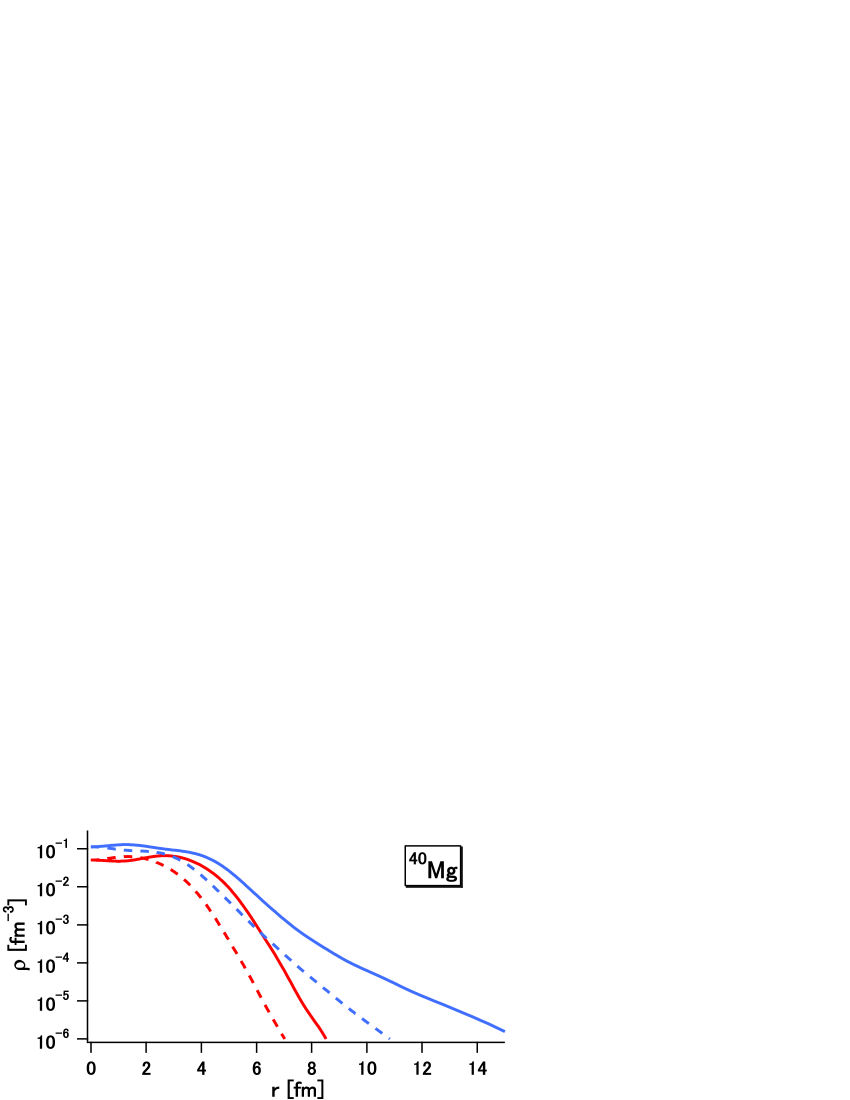
Figure 3: Proton (in red color) and neutron (in blue color) densities of ⁴⁰Mg in the $x$ (dashed lines) and the $z$ (solid lines) directions, calculated with the D1S interaction.

To observe the shape of ⁴⁰Mg at low density, equi-density lines on the $xz$-plane are drawn in Fig. 4. For comparison, similar plots for ²⁴Mg and ³⁴Mg are given as well. All the three Mg nuclei have prolate deformation in the present HF calculation. The equi-density lines distribute with almost equal intervals from $10^{-2}$ to $10^{-6}\,\mathrm{fm}^{-3}$, indicating exponential decrease of $\rho_{\tau}$. With the exception of $\rho_{n}$ in ⁴⁰Mg, the size of the intervals does not depend on direction. Although the $\rho_{\tau}=10^{-6}\,\mathrm{fm}^{-3}$ line in ²⁴Mg is slightly constricted in the $x$ direction, it could be influenced by deviation from the exponential asymptotics due to numerical errors. The contour plot of $\rho_{n}$ in ⁴⁰Mg is intriguing. The large intervals of the equi-density lines correspond to the slow damping of $\rho_{n}$ due to the small $\varepsilon_{\!F}$. However, the intervals are comparable to those in ³⁴Mg in the $x$ direction. We view the neck structure in the low $\rho_{n}$ region.

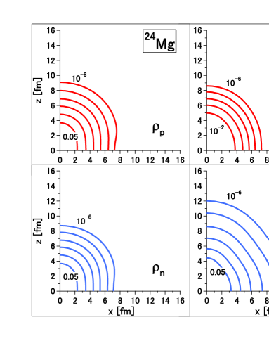
Figure 4: Contour plot of $\rho_{\tau}$ ($\tau=p,n$) on the $xz$-plane for ²⁴Mg, ³⁴Mg and ⁴⁰Mg, calculated with the D1S interaction. Positions of $\rho_{\tau}=0.05$, $10^{-2}$, $10^{-3}$, $10^{-4}$, $10^{-5}$ and $10^{-6}\,\mathrm{fm}^{-3}$ are presented.

Because it mixes the $m_{\ell}=0$ and $1$ components, the pair correlation tends to restore the spherical symmetry in the density distribution in the asymptotic region. Depending on degree of the mixing, the neck structure may survive or disappear. However, in the present HFB calculation with the D1S interaction, we do not find a superfluid solution having lower energy than the HF minimum in ⁴⁰Mg. Thus the density distribution of ⁴⁰Mg shown in Figs. 3 and 4 is not altered.

If the $\ell\geq 2$ components remain sizable in the asymptotic region, deformed halos (including neck structure) with other $(\pi,m)$ may be present. In Ref. [19], possibility of deformed halos depending on the direction was pointed out for ¹¹Be and ¹³C, based on the Skyrme HFB calculations. Those halos are formed by a $(\pi,m)=(+,1/2)$ orbit.

There remain problems with respect to deformed halos: (a) how correlations beyond HFB (including restoration of the rotational symmetry) affect them, and (b) whether they are detectable in experiments. Although both questions are very important, it is not easy to give satisfactory answers at this moment and we leave these problems to future studies. We here emphasize that such exotic structure of nuclear halos can be investigated only via numerical methods that are capable of describing the wave-function asymptotics appropriately.

5 Summary

We extensively develop a new method of implementing the Hartree-Fock (HF) and the Hartree-Fock-Bogolyubov (HFB) calculations of nuclei with deformation, applying the Gaussian expansion method (GEM). Owing to the adaptability in describing radial degrees of freedom, which is confirmed by the HF calculations from ¹⁶O to ²⁰⁸Pb, we adopt the spherical GEM bases. We argue how large $\ell$ should be taken into account, by comparing the numerical solutions obtained from the spherical GEM bases with the analytic ones in the axially deformed harmonic oscillator. The present method maintains three notable advantages of the GEM algorithm for the mean-field calculations: (i) we can efficiently describe the energy-dependent asymptotics of single-particle (s.p.) wave functions at large $r$, (ii) we can handle various effective interactions, including those having non-locality, and (iii) a single-set of bases is applicable to wide mass range of nuclei and therefore is suitable to systematic calculations.

The present method is applied to magnesium nuclei with the Gogny force. We show that the present results are no worse than those in the literatures, from the variational viewpoint. Compared with the conventional method using the harmonic oscillator bases, the present method is suitable particularly to nuclei far from the $\beta$ stability. For ⁴⁰Mg, we suggest neck structure of a neutron halo, which arises due to the asymptotic behavior depending on the direction. Such a possibility can be argued only via methods describing the asymptotic form of the s.p. wave functions appropriately.

This work is financially supported in part as Grant-in-Aid for Scientific Research (C), No. 19540262, by Japan Society for the Promotion of Science. Numerical calculations are performed on HITAC SR11000 at Institute of Media and Information Technology, Chiba University, and at Information Technology Center, University of Tokyo.

References

- [1] H. Nakada and M. Sato, Nucl. Phys. A699 (2002) 511; ibid. A714 (2003) 696.
- [2] H. Nakada, Nucl. Phys. A764 (2006) 117; ibid. A801 (2008) 169.
- [3] M. Kamimura, Phys. Rev. A 38 (1988) 621.
- [4] E. K. Warburton, J. A. Becker and B. A. Brown, Phys. Rev. C 41 (1990) 1147.
- [5] M. Yamagami and N. Van Giai, Phys. Rev. C 69 (2004) 034301.
- [6] E. Hiyama, Y. Kino and M. Kamimura, Prog. Part. Nucl. Phys. 51 (2003) 223.
- [7] J. F. Berger, M. Girod and D. Gogny, Comp. Phys. Comm. 63 (1991) 365.
- [8] H. Nakada, Phys. Rev. C 68 (2003) 014316.
- [9] A. Bohr and B. R. Mottelson, Nuclear Structure vol. 1 (Benjamin, New York, 1969), p. 220.
- [10] J. Dechargé and D. Gogny, Phys. Rev. C 21 (1980) 1568.
- [11] R. Blümel and K. Dietrich, Nucl. Phys. A471 (1987) 453.
- [12] Y. Sugawa, M. Kimura and H. Horiuchi, Prog. Theor. Phys. 106 (2001) 1129.
- [13] R. Rodríguez-Guzmán, J. L. Egido and L. M. Robledo, Phys. Lett. B 474 (2000) 15.
- [14] T. Misu, W. Nazarewicz and S. Åberg, Nucl. Phys. A614 (1997) 44.
- [15] I. Hamamoto, Phys. Rev. C 69 (2004) 041306.
- [16] J. Terasaki, H. Flocard, P.-H. Heenen and P. Bonche, Nucl. Phys. A621 (1997) 706.
- [17] R. Rodríguez-Guzmán, J. L. Egido and L. M. Robledo, Nucl. Phys. A709 (2002) 201.
- [18] T. Baumann et al., Nature 449 (2007) 1022.
- [19] J. C. Pei, F. R. Xu and P. D. Stevenson, Nucl. Phys. A765 (2006) 29.