Optimal control of electromagnetic field using metallic nanoclusters

Abstract

The dielectric properties of metallic nanoclusters in the presence of an applied electromagnetic field are investigated using non-local linear response theory. In the quantum limit we find a non-trivial dependence of the induced field and charge distribution on the spatial separation between the clusters and on the frequency of the driving field. Using a genetic algorithm, these quantum functionalities are exploited to custom-design sub-wavelength lenses with a frequency controlled switching capability.

Introduction: Recently we developed a theory that describes the non-local linear dielectric response of nano-metal structures to an externally applied electric field levi . Unlike conventional phenomenological classical theory mie , we are able to model the transition from classical to quantum response as well as the coexistence of classical and quantum response in structures of arbitrary geometry. This is of some practical importance because metallic nanoclusters can now be made sufficiently small such that non-local effects due to finite system size and cluster shape dominate the spectral response. In particular, when the ratio between the smallest characteristic length scale and the Fermi wavelength is comparable to or smaller than unity, these systems can fail to fully screen external driving fields. Also, in the quantum limit one needs to take into account discreteness of the excitation spectrum as well as the intrinsically strong damping of collective modes. Our model captures these single and many particle quantum effects.

In this paper we report on studies in which we explore optimal design of nanoscale metallic structures to control electromagnetic field intensity on subwavelength scales. We are motivated by the non-intuitive nature of quantum response and the potential for applications such as surface enhanced Raman scattering sers ; nurmikko .

Model: To capture the single-particle and collective aspects of light-matter interaction in inhomogeneous nanoscale systems one should consider non-local response theory in the quantum regime levi . The Schrödinger equation for noninteracting electrons with mass $m_{\text{e}}$ and charge $e$ moving in a potential $V(\mathbf{r})$, is given by

$$H\Psi_{i}(\mathbf{r})=\left(-\frac{\hbar^{2}}{2m}\nabla^{2}+V(\mathbf{r})\right)\Psi_{i}(\mathbf{r})=E_{i}\Psi_{i}(\mathbf{r}).$$ (1)

This equation must be solved simultaneously with the Poisson equation to determine the local potential due to the spatial distribution of the positive background charges. Using the jellium approximation, the resulting potential is implicitly given by $\nabla^{2}V(\mathbf{r})=4e\pi\rho(\mathbf{r})$, where the density of the positive background charge $\rho(\mathbf{r})$ satisfies the condition of neutrality, so that $\int\rho(\mathbf{r})d\mathbf{r}=N_{\text{el}}$, where $N_{\text{el}}$ is the number of electrons. The induced potential $\phi_{\text{ind}}$ is then determined from the self-consistent integral equation

$$\phi_{{\text{ind}}}({\bf r},\omega)=\int{{\frac{\chi({\bf r^{\prime}},{\bf r^{\prime\prime}},\omega)\phi_{{\text{tot}}}({\bf r^{\prime\prime}},\omega)}{{\left|{{\bf r}-{\bf r^{\prime}}}\right|}}d{\bf r^{\prime}}}d{\bf r^{\prime\prime}}}.$$ (2)

Here $\chi({\bf r^{\prime}},{\bf r^{\prime\prime}},\omega)$ is the non-local density-density response function, and $\phi_{\text{tot}}(\mathbf{r},\omega)=\phi_{\text{ext}}(\mathbf{r},\omega)+\phi_{\text{ind}}(\textbf{r},\omega)$ is the self-consistent total potential. The induced field is found via $\mathbf{E}_{{\text{ind}}}(\mathbf{r},\omega)=-\mathbf{\nabla}\phi_{{\text{ind}}}(\textbf{r},\omega)$. The external field is assumed to be harmonic, with frequency $\omega$, linearly polarized, and with the wavelength much larger than the characteristic system’s size. The integral equation is discretized on a real-space cubic mesh with lattice constant $L$. Its natural energy scale $E_{0}$ is defined by $E_{0}=\hbar^{2}/(2m_{\text{e}}L^{2})$, and the resulting system of linear equations can be solved numerically. The damping constant which determines the level broadening is set to $\gamma=2\times 10^{-3}$ $E_{0}$.

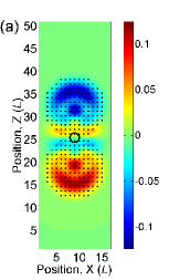
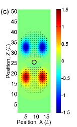
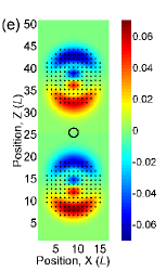
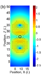
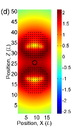
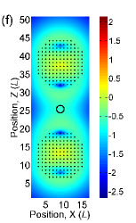
Figure 1:  The direction of the static external field $\mathbf{E}_{\text{ext}}(\omega=0)$ points along the $z$ axis. Induced charge density (upper row) and corresponding induced electric field $\log_{10}(|\mathbf{E}_{\text{ind}}(x,0,z)|^{2})$ (lower row) in systems of two conducting spherical clusters with radii $R=7L$ (shown by black dots), where $L$ is the lattice spacing. The plots show top views of the three-dimensional systems. The relative distance $D$ between the two closest points of the spheres is varied from left to right: (a),(b): $D$=0; (c),(d): $D=4L$, (e),(f): $D=13L$. $N_{\text{el}}=20$ for the system, temperature $T$=0 K and damping constant $\gamma=2\times 10^{-3}$ $E_{0}$. The target volume over which the field intensity is to be maximized is indicated as a circle of radius $L$ at the system center.

Static Case: To gain better understanding and intuition into the dielectric response of nanoscale clusters in the quantum limit, let us first consider systems consisting of two identical nanospheres with a total number of electrons $N_{\text{el}}$ and separated by an adjustable distance $D$ (top view shown in Fig. 1). The nanospheres are placed in a static electric field, and the z-direction of the external field is aligned along the line connecting the sphere centers. Our goal is to maximize the intensity of the induced electric field $W_{\text{int}}=\int_{V_{0}}|\mathbf{E}(\mathbf{r})|^{2}d\mathbf{r}$ in a target volume of radius $R_{\text{V}}=L$, centered between the two clusters, by varying the cluster separation $D$. In the regime of large electron densities, classical theory predicts that $W_{\text{int}}$ diverges as the spheres approach each other, i.e. $W_{\text{int}}\to\infty$ as $D\to 0$, and hence the spherical clusters would need to be as close as possible to each other to maximize the induced field in the target area. As seen in Fig. 1, this is no longer true for small carrier concentrations (here $N_{\text{el}}=20$), in which case quantum fluctuations strongly influence the electromagnetic response. For sufficiently small separations (Fig. 1(a) and (b)) the entire system responds as a single dipole (with small corrections at the interface between the two clusters). The charge density distribution depicted in Fig. 1(a) shows charge polarization (red: positive, blue: negative) along the applied field, whereas the corresponding induced electric field in Fig. 1(b) remains relatively homogeneous throughout the entire system. Remarkably, as shown in Fig. 1(c) and (d), there are finite optimum separations between the spheres which maximize the induced field at the center between them. As will become apparent, the physical reason for this is quantum wave functions constrain accessibility to geometric features. For the parameters chosen in this example, $D_{\mathrm{opt}}\approx 4L$ occurs at the threshold separation distance beyond which the two clusters cease to act as a single dipole. It is evident from Fig. 1(d) that at this resonance condition the overall induced field intensity is highly inhomogeneous and peaks at two orders of magnitude larger compared to off-resonance conditions. Moreover, there can be further such resonances, e.g. at $D_{\mathrm{opt}}\approx 7L$ for the present parameters, which maximize the induced field intensity in between the nanospheres. As observed in Fig. 1(e) and (f), for larger distances $D$ one can ultimately treat the spheres as independent dipoles, for which the induced field energy $W_{\text{int}}$ scales as $D^{\lambda}$, with $\lambda=-8$, which we have verified numerically footnote1 .

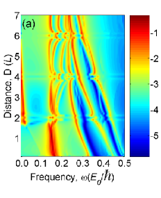
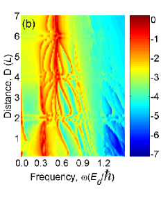
Figure 2: Landscapes of the induced electric field energy $\log_{10}(W_{\text{ind}})$ in systems of two conducting nanospheres with radii $R=7L$ as a function of the frequency of the external field $\omega$ and the cluster separation distance $D$, measured between the two closest points of the nanospheres. The direction of the external field points along the line connecting the sphere centers, damping constant $\gamma=2\times 10^{-3}E_{0}$. (a) $N_{\text{el}}=20$, (b) $N_{\text{el}}=100$.

Dynamic Screening: Although the characteristic Thomas-Fermi screening length is known to increase with decreasing carrier concentration, this quantity only describes the screening of slowly varying potentials. The lower the carrier concentration, the worse the system screens rapidly varying potentials. For relatively small electron densities the screening length becomes comparable with the distance between the spheres $D$. Thus, sensitivity of the response of the system to carrier concentration suggests strong effects of carrier screening. This will be most pronounced in the region between the spheres, where the potential undergoes significant changes. To illustrate how the carrier concentration in the nanospheres dramatically changes the dynamic dielectric response of the system, we show in Fig. 2 plots of $W_{\text{int}}$ as a function of the frequency of the external field and relative distance $D$ between the spheres. In Fig. 2(a) we consider the case of the same low carrier concentration as in Fig. 1. There are $N_{\text{el}}=20$ electrons in the system, with a characteristic Fermi wavelength $\lambda_{\text{F}}\approx 3L$, which is the same order of magnitude as the radii of the spherical clusters. The various observed resonances correspond to excitations of different geometric modes available in the discrete spectrum of the system (dipole-dipole, quadruple-quadruple, etc). For the parameters chosen in Fig. 2(a), the dominant geometric resonances occur at frequencies less than $\hbar\omega=0.2E_{0}$. Interestingly, there is no zero-frequency peak at $D\approx 0$, which is in stark contrast to the case of denser fillings that correspond to the classical limit, e.g. as shown in Fig. 2(b). At low fillings, the delocalized charge density response results in less efficient screening in the region between the clusters, and hence the system of two clusters responds as a whole. This significantly reduces the magnitude of the induced charge densities near the closest surfaces of the spheres and limits the maximum possible value of $W_{\text{int}}$. Moreover, quantum discreteness of the energy levels results in a non-monotonic dependence of $W_{\text{int}}$ on $D$, which in turn leads to the non-zero optimal distance $D_{\text{{opt}}}$, discussed above. Note, that for the parameter set chosen here at a finite frequency $\omega=0.1E_{0}$ the optimal distance is near $D=0$, i.e. similar to the static response of the classical system. In Fig. 2(b) we consider the same system parameters but at a higher carrier concentration, i.e. $N_{\text{el}}=100$ electrons. The corresponding characteristic Fermi wavelength is $\lambda_{\text{F}}\approx 1L$, which allows the dielectric response of the system to be much closer to the classical limit. In this case many more geometric resonances are observed compared to the low-filling regime (Fig. 2(a)). Also, in contrast to the quantum limit these resonances depend more strongly on changes in separation $D$ and converge into a single dominant peak at $\hbar\omega\approx 0.72$$E_{0}$ for $D\geq 7$$L$. Also note the large maximum of $W_{\text{int}}$ at $D\approx 0$ and $\omega\approx 0$, as it is expected for the static limit in the classical regime.

Optimal Design (static): The above example illustrates that there can be significant differences between the dielectric response in the classical and quantum regimes. Let us now explore how the quantum functionality of such structures can in principle be used for the design of nanoscale devices. In the following, we pursue an optimal design problem of a prototype system with multiple adjustable parameters, using a numerical global optimization technique based on the genetic algorithm thalken . Specifically, we wish to optimize a system containing $5$ point-like charges with $q=+4e$ each. In order to reduce the complexity of the problem the charges are placed on a line along the $z$ axis, and we optimize the $z$ coordinates of the placed charges. This reduces the optimization problem to $5$ parameters. A static external electric field is applied along the $z$ axis. In order to discretize the numerical search space, the positions of the charges are restricted to be on a lattice with lattice constant $L$. We search for optimal configurations of the charges that maximize the induced field intensity in a target region $V_{0}$, located at the center of the system at $z=1/2L_{\mathrm{tot}}$. Here $L_{\mathrm{tot}}$ is the total length of the optimization box along the $z$ direction. The total number of electrons in the system $N_{\text{el}}=20$ is chosen to insure the system’s response to be in the quantum regime. It usually takes about $1100$ seconds to perform optimization on a 20 node cluster configured with two 1GHz processors per node.

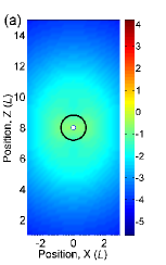
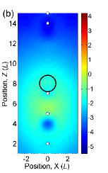
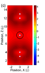
Figure 3: Induced field intensity $\log_{10}(|\mathbf{E}_{\text{ind}}(x,0,z)|^{2})$ for different configurations of scatterers: five point-like charges with $q=+4e$ (marked by white dots), each is placed along a line on the z-axis, parallel to the external field. $N_{\text{el}}=20$ and $\gamma=2\times 10^{-3}E_{0}$. (a) All charges are placed at the center, (b) a random configuration, (c) optimized configuration with target to yield maximum intensity of induced field.

In Fig. 3(a) the intensity of the induced field is shown for the case of all the point charges placed at the center of the target area, as it would be suggested by classical intuition. While the induced field is indeed largest at the system center, the overall intensity is relatively small compared to optimized configurations. For purposes of comparison, in Fig. 3(b) we also show the intensity of the induced field for a random configuration of point charges. In contrast to Figs. 3(a,b), Fig. 3(c) displays the induced field for a numerically optimized configuration of point charges. In agreement with the examples in Figs. 1 and 2(a), the optimal distance between the placed charges is finite. The optimization algorithm finds a compromise between the distance to the system center and the inter-particle distances of the point charges that maximizes the induced charge density. This is achieved via maximization of the induced charge localization in the quantum system, leading to the most efficient screening near the target volume. Thus, we find that using a genetic algorithm it is possible to create highly efficient optimized structures with broken spatial symmetries which function as a sub-wavelength lens for electromagnetic radiation. Note also that the optimal configuration in Fig. 3(c) has an inversion symmetry about the system center which arises naturally during the optimization procedure. Comparing the optimized result with the classical configuration (Fig. 3(a)) and the random configuration (Fig. 3(b)), it is evident that the optimal configuration leads to a field intensity in the focal region that is four orders of magnitude larger. We have performed further optimizations for the positions of 2-8 point-like charges with the same target functionality. Significant even-odd effects are observed in the optimal arrangements. For even numbers of charges, none of the charges should be placed in the system center, whereas for odd numbers of charges the optimal configuration consists of two symmetrically arranged equal groups of charges, and one charge is placed in center of the target area.

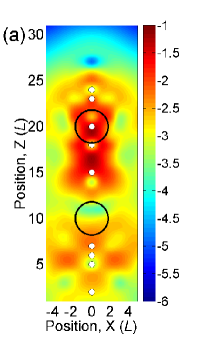
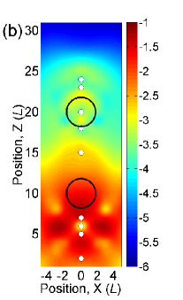
Figure 4:  “Frequency splitter”: induced field intensities $\log_{10}(|\mathbf{E}_{\text{ind}}(x,0,z)|^{2})$ for optimized configurations with $N_{\text{el}}=20$ electrons and $10$ moving scattering centers (marked by white dots). Note that two moving centers are overlapping at $z=5L$. We use $\gamma=2\times 10^{-3}E_{0}$, the external field points along the $z$ direction. (a) $\hbar\omega_{1}=0.09E_{0}$, (b) $\hbar\omega_{2}=0.130E_{0}$.

Optimal Design (dynamic): Finally, let us consider the case of time-varying fields, with the goal to design a “frequency splitter” in the sub-wavelength limit. In this example we again allow the point-like charges to be placed along the $z$ axis, and search for optimal spatial configurations of the charges which maximize the induced field intensity in a target volume centered at $z=2/3L_{\mathrm{tot}}$ for a field frequency $\omega_{1}$, and in a second target volume centered at $z=1/3L_{\mathrm{tot}}$ for a second field frequency $\omega_{2}$. Numerical optimization was performed for $10$ moving positive background charges with $q=+2e$ each and $N_{el}=20$ electrons in the system. In Fig. 4, we show the induced field intensity for optimized configurations of charges with two different frequencies (a) $\hbar\omega_{1}=0.09E_{0}$ and (b) $\hbar\omega_{2}=0.130E_{0}$. The selectivity of this device can be quantified by the induced field energies $W_{1}$ and $W_{2}$ in the target volumes $1$ and $2$ correspondingly, and their ratio at two distinct frequencies $\omega_{1}$ and $\omega_{2}$. We find that for the optimized configuration the ratio $W_{1}/W_{2}\approx 0.09$ at $\omega_{1}$, and $W_{2}/W_{1}\approx 0.07$ at $\omega_{2}$.

Conclusions:

In summary, the dielectric properties of spherical nanoclusters in their quantum regime offer a richness of functionalities which is absent in the classical case. These include a highly non-trivial screening response and dependence on the frequency of the driving field. Intuition based on classical field theory, e.g. divergence of induced field in the static limit as the distance between the spheres decreases, breaks down, and can thus not be relied on for the design of new atomic-scaled devices. In particular, one cannot expect to induce localized charge density distributions with a characteristic length scale much smaller than the typical Fermi wavelength of the system and collective excitation can be dramatically modified. Moreover, in the quantum regime the delocalized induced charge densities can provide increased robustness of the optimized quantity, and thus decrease the complexity of optimal design. Quantum mechanical effects were also found to set boundaries on the maximum values of target quantities, i.e. induced field intensity in the system. Using genetic search algorithms, we have demonstrated that optimal design can lead to field intensities orders of magnitude larger than “simple” guesses based on intuition derived from classical theory.

For applications such as surface enhanced Raman scattering, the electric field enhancement in the nm surrounding the molecule depends critically on the local configuration of both the metallic particle and the molecule. In principle, optimal particle shapes can be found that maximize Raman activity for a given molecule attached to the metal surface. The approach discussed in this paper opens new possibilities for applications. For example, it should be feasible to use our theory in combination with search algorithms to create robust and reliable highly Raman active nano-structured surfaces.

Acknowledgements: We are grateful to Pinaki Sengupta for fruitful discussions, and acknowledge support by the DOE under grant DE-FG02-05ER46240. The simulations were carried out at the high-performance computing computing center at USC. This work was performed under the auspices of the National Nuclear Security Administration of the U.S. Department of Energy at Los Alamos National Laboratory under Contract No. DE-AC52-06NA25396 and supported by DARPA and ONR.

References

- (1) I. Grigorenko, S. Haas and A.F.J. Levi, Phys. Rev. Lett. 97, 036806 (2006).
- (2) G. Mie, Annalen der Physik, 25, 377 (1908).
- (3) S. Nie and S. R. Emory, Science 275, 1102 (1997).
- (4) T. Atay, J.H. Song, and A.V. Nurmikko, Nano Lett. 4, 1627 (2004).
- (5) Consider a system of four charges: at positions , , and at positions , . The field intensity at position () is , yielding asymptotics.
- (6) J. Thalken, W. Li, S. Haas, and A.F.J. Levi, Appl. Phys. Lett. 85, 121 (2004).