Analysis of nucleus-nucleus collisions at high energies and Random Matrix Theory

Abstract

We propose a novel statistical approach to the analysis of experimental data obtained in nucleus-nucleus collisions at high energies which borrows from methods developed within the context of Random Matrix Theory. It is applied to the detection of correlations in a system of secondary particles. We find good agreement between the results obtained in this way and a standard analysis based on the method of effective mass spectra and two-pair correlation function often used in high energy physics. The method introduced here is free from unwanted background contributions.

I Introduction

There is currently an enormous effort underway to detect signals of possible transitions between different phases of strongly interacting matter produced in high energy nucleus-nucleus collisions (cf 1 ; 2 ). It is expected that in central collisions, at energies that are and will be soon available at CERN Super Proton Synchrotron (SPS), BNL Relativistic Heavy Ion Collider (RHIC), and CERN Large Hadron Collider (LHC), the nuclear density may exceed by a few orders of magnitude the density of stable nuclei. At such extreme conditions one would expect that a final product of heavy ion collisions could present a composite system that consists of free hadrons, quarks and gluons. However, quarks and gluons cannot be unambiguously identified with present detectors. In addition, the identification, for example, of a quark-gluon plasma is hindered due to a multiplicity of secondary particles created at these collisions. In fact, there are numerous additional mechanisms of particle creation that mask the presence of a quark-gluon plasma. A natural question arises as to how to identify a useful signal that would be unambiguously associated with a certain physical process?

Amongst the most popular traditional methods of analysing data produced at high-energy nucleus-nucleus collisions are: i) the correlation analysis drem , ii) the analysis of missing masses b2 and effective mass spectra b4 , iii) the interference method of identical particles pod etc. It is currently believed that by measuring event-by-event fluctuations it would be possible to observe anomalies from the onset of deconfinement mr . Often though, results based on such methods are sensitive to assumptions made concerning the background measurements and mechanisms included in the corresponding model. For example, one of the popular approaches to studying particle production in heavy ion collisions is through statistical mechanics techniques (cf a ; b ; c ). However, recent theoretical analyses of the multiplicity fluctuations demonstrate that corresponding results are different in different ensembles and it is sensitive to conservation laws obeyed by a statistical system beg .

Transport theory has played an important role in the interpretation of experimental results in heavy ion reactions at various energy domains (see, for example, Refs.bass, ; bord, ). The underlying concept of transport models is based on numerical solution of the Boltzmann equation (the Vlasov-Uehling-Uhlenbeck, the Boltzmann-Uehling-Uhlenbeck (BUU) etc). However, exact numerical solutions, for example, of the BUU equation are very difficult to obtain and, therefore, various approximate treatments have been developed bass ; bord . Up to now there are no stringent proofs that such approximations really yield a solution of the full transport problem. The only proof is that numerical solutions provide the asymptotic limit at equilibrium, which can be deduced from the Boltzmann equation (the BUU equation without potential and Pauli-blocking factor) (see details in Ref.bass, ). We recall that the BUU equation is a generalization of the Fokker-Planck equation associated with the Brownian motion of particles in a classical Coulomb gas model. Dyson discovered that this model can be described well in terms of the Gaussian ensembles of the Random Matrix Theory (RMT) meh . This fact implies that one might expect that the RMT could be useful for analysis of experimental results obtained in heavy ion reactions at high energies.

The RMT was originally introduced to explain the statistical fluctuations of neutron resonances in compound nuclei P65 (see also Ref. Brody, ). There the precise heavy-compound-nuclear Hamiltonian is unknown or rather poorly known, and there is a large number of strongly interacting degrees of freedom. Wigner first suggested replacing it by an ensemble of Hamiltonians which describe all possible interactions Wigner . The theory assumes that the Hamiltonian belongs to an ensemble of random matrices that are consistent with the fundamental symmetries of the system. In particular, since the nuclear interaction preserves time-reversal symmetry, the relevant ensemble is the Gaussian Orthogonal Ensemble (GOE). Whereas if time-reversal symmetry were broken, the Gaussian Unitary Ensemble (GUE) would be the relevant ensemble. The GOE and GUE correspond to ensembles of real symmetric matrices and of complex Hermitian matrices, respectively.

It is noteworthy that during the last twenty years the RMT grew into the powerful new statistical theory of fluctuations in a variety of physical problems. For example, the RMT has become a very successful theoretical method for analysing fluctuation properties found in the data from atoms and nuclei, quantum dots, and many other systems (see, for example, Ref.Gur, ). In various fields, the Dyson-Mehta statistical measures are the most often used to quantify a system’s correlations and to determine what information the fluctuations contain. They can be used with any discrete data to search for correlations. These measures do not depend on the background of measurements and used in the context of RMT give universal forms depending only on the fundamental symmetries preserved. Their only requirement is that local mean densities (or secular behaviors) be understood and their effects be removed. Furthermore, a change of fluctuation properties of a system under consideration, induced by a change its symmetry properties, can be detected by the RMT tools unambiguously (see below). Therefore, these tools could provide a way of detecting the transition between different phases (with different fluctuation properties) of strongly interacting matter produced in high energy nucleus-nucleus collisions.

The main aim of the present paper is to introduce the Dyson-Mehta statistical measures for analysis of experimental data from nucleus-nucleus collisions at high energies in order to detect effects produced by correlations. More specifically, to demonstrate that they are very sensitive to spacing correlations present in the nucleus-nucleus collision data, and serve a useful purpose of independent complementary approach to the standard tools designed for such an analysis in high energy physics. Note, in general, the standard tools are based on different concepts, in contrast to the Dyson-Mehta measures that are formulated within unique, mathematically rigorous theory. In Section II we review how to detect the manifestation of correlations with the aid of nearest neighbor spacing distribution (NND) from the data obtained in light nuclei collisions in Dubna experiments. To check the validity of our findings by dint of the NND in Section III we analyse the same data within the method of effective mass widely used in the analysis of data from nucleus-nucleus collisions at high energies. Section IV is devoted to analysis of density-density correlations based on the Dyson-Mehta statistical measures and the two-pair correlation function often used in high energy physics. The main conclusions are summarized in Section V. The preliminary results of our analysis were presented in sh1 .

II Nearest-neighbor spacing distribution

II.1 Some experimental details

To demonstrate the feasibility of using the Dyson-Mehta statistical measures in the context of high energy nuclear collisions, we make use of the experimental data that have been obtained with the 2-m propane bubble chamber of High Energy Physics Laboratory (LHE), JINR [8] ; [9] ; int3 . The chamber, placed in a magnetic field of 1.5 T, was exposed to beams of light relativistic carbon nuclei at the Dubna Synchrophasotron. Nearly all secondary particles, emitted in a 4$\pi$ total solid angle, were detected in the chamber.

Figure 1: The momentum distribution of the secondary charge particles.

All negatively charged particles, except those identified as electrons, are considered as $\pi^{-}$-mesons. The contamination from misidentified electrons and negative strange particles does not exceed 5$\%$ and 1$\%$, respectively. On Fig.1 the momentum distribution $dN/d|p|$ of the secondary charged particles is displayed. The maximum of the particle production is observed at $|p|\sim 0.5-0.7$ GeV/c. The particle momenta were calculated from the particle trajectories in a magnetic field taking into account ionization and radiation losses. In particular, the uncertainty in the momentum value were estimated taking account of the effects of multiple Coulomb scattering and bremsstrahlung radiation. The average uncertainty in the momentum and the angle measurements varies as: $\langle\Delta p/p\rangle=(11.5\pm 0.3)\%$, $\langle\Delta\theta\rangle\sim 0.8^{0}$. The minimum momentum for pion registration is about 70 MeV/c in lab frame (we consider all kinematic variables in the lab frame). The protons were selected by a statistical method applied to all positive particles with a momentum of $|p|>500$ MeV/c (slow protons with $|p|\leq 700$ MeV/c were identified by ionization in the chamber).

In this experiment, there are 37792 ¹²C+¹²C interaction events at a momentum of 4.2A GeV/c (for greater discussion of the details see [9] ; int3 ; [9a] ) containing 7740 events with more than ten tracks of charged particles. The separation method of ¹²C+¹²C collisions in propane ($C_{3}H_{8}$), data processing, identification of particles and discussion of corrections are described in detail in [10] . About 70$\%$ of ¹²C+¹²C events have been identified with the aid of this method. The set residue of events was separated statistically between carbon+carbon and carbon+hydrogen collisions with the aid of the event ”weight”. The ”weights” were estimated from known cross sections for inelastic carbon+carbon and carbon+hydrogen collisions.

II.2 Basic remarks

If one supposes that the momenta of secondary particles produced in nucleus-nucleus collisions may be treated in analogy with eigenstates of a composite system, just like the eigenstates of the compound nucleus, then the statistical analysis methods P65 introduced by Dyson and Mehta can be applied to the LHE collision data. By analogy with compound nuclei discussed in the Introduction, one may assume that the observed spectra (Fig.1) belong to the effective QCD Hamiltonian which describes the composite system, but is unknown. We point out that the secondary particle momenta are well determined in the experiment. It is, therefore, natural to use the momentum as a proper variable for our analysis in order to avoid possible errors at the transformation from the momentum to the energy, which requires an accurate determination of the corresponding mass value.

Figure 2: Nearest-neighbor spacing momentum distribution (histogram) p(s) for different regions of measured momenta: (a) and (b) correspond to $0.15<|p|<1.14$ GeV/c; (c) and (d) correspond to $1.14<|p|<4.0$ GeV/c; (e) and (f) correspond to $4.0<|p|<7.5$ GeV/c. The total distribution (it includes data related to all charged secondary particles) consists in (a), (c), and (e) panels. The distribution for proton momenta consists in (b), (d), and (f) panels. The Poisson and the Wigner surmise distributions are connected by dot-dashed and solid lines, respectively.

Based on this supposition, the ordered sequence of “energy levels” $\{E_{i}\},i=1,...,N$ comes from the ordered sequence of the detected momenta of the secondary particles. Hereafter, for the sake of convenience we associate a symbol ”E” with an absolute value of the momentum $|p|$. To analyse the statistical fluctuations of the spectrum $\{E_{i}\}$, it is necessary to separate its smoothed average part whose behaviour is nonuniversal and cannot be described by the RMT boh2 . A separation of fluctuations of a quantum spectrum can be based on the analysis of the density of states below some threshold $E$

$$\rho(E)=\sum_{i=1}^{N}\delta(E-E_{i})\,.$$ (1)

We can define a staircase function

$$S(E)=\int_{-\infty}^{E}\rho(E^{\prime})dE^{\prime}=\sum_{i=1}^{N}\theta(E-E^{\prime}),$$ (2)

giving the number of points on the momentum axis which are below or equal to $E($or $|p|)$. Here

$$\theta(x)\,=\,\left\{\begin{array}[]{l}0\qquad\,for\,\,\,x<0\\ 1\qquad\,for\,\,\,x>1\\ \end{array}\right.$$ (3)

We separate $S(E)$ in a smooth part $\zeta(E)$ and the reminder that will define the fluctuating part $S_{\rm fl}(E)$

$$S(E)=\zeta(E)+S_{\rm fl}(E),$$ (4)

such that the integral of $S_{\rm fl}(E)$ is zero. Here, the smooth function $\zeta(E)$ gives the mean number of eigenvalues less than or equal to $E$ of the exact eigenvalue distribution $S(E)$. The smooth part $\zeta(E)$ can be determined either from semiclassical arguments or by using a polynomial/spline interpolation for the exact staircase function. From this sequence a new one is obtained by the unfolding procedure of the original spectrum $\{E_{i}\}$ through the mapping $E\rightarrow x$ (see details in Sec.II.3)

$$x_{i}=\zeta(E_{i}),\qquad i=1,...,N\,.$$ (5)

The effect of the mapping is that the sequence $\{x_{i}\}$ has on average a constant mean spacing (or a constant density), irrespective of the particular form of the function $\zeta(E)$ boh2 . Note that there is no any combinatorics involved in a such procedure. That which remains in the sequence are the fluctuations away from unit mean. Next, one defines the spacing $s_{i}=x_{i+1}-x_{i}$ between two adjacent points. Collecting ${s_{i}}$ in a histogram, one obtains the probability density or the NND. We stress that, in general, this procedure does not involve any uncertainty or spurious contributions and deals with a direct processing of physical data.

Bohigas et al Boh conjectured that the RMT describes the statistical fluctuations of a quantum system whose classical dynamics is chaotic. Quantum spectra of such systems manifest a strong repulsion (anticrossing) between quantum levels, while in non-chaotic (regular) systems crossings are a dominant feature of spectra. In turn, the crossings are usually observed where there is no mixing between states that are characterized by different good quantum numbers, and the anticrossings signal a strong mixing due to a perturbation brought about by either external or internal sources (cf Refs.P65, ; Brody, ).

Thus, if the ”events” $\{x_{i}\}$ are independent, i.e., correlations in the system under consideration are absent, the form of the histogram must follow $p(s)=\exp(-s)$ known as the Poisson density. On the other hand, if the levels are repelled (anticorrelated) as in the GOE, the density is approximately given by the Wigner surmise form $p(s)=\frac{\pi}{2}s\exp(-\frac{\pi}{4}s^{2})$. In other words, any correlations that produces the deviation from the regular pattern (Poisson distribution): production of a collective state (resonance), or some structural changes in the system under consideration would be uniquely identified from the change of the histogram shape. In particular, the transition from one probability density to the other has been used in nuclear structure physics to study the stabilization of octupole deformed shapes and transition from the chaotic to the regular pattern in the classical limit H94 . Therefore, such an analysis can provide the first hint of some structural changes at different parameters of the system under consideration, in particular, in different energy (momentum) intervals.

II.3 The experimental NND histograms

In order to reveal structural changes in the momentum distribution we determine the smooth part $\zeta(E)$ using a polynomial function of the fifth order to interpolate the exact staircase function (see also Eq.(4)):

$$\zeta(E)=\sum_{k=0}^{5}a_{k}E^{k},$$ (6)

where $E=|p|$ are the experimental momentum values in the given event. We recall that momenta are ordered in ascending series. The parameters $a_{k}$ were optimized with the aid of the program MINUIT. Next, we obtain a new spectra $\{x_{i}\}$ by the unfolding procedure of the original spectrum $\{E_{i}\}$ through the mapping $E\rightarrow x$ by means of the polynomial function (6) with the optimized coefficients $a_{k}$: $x_{i}=\zeta(E_{i}),i=1,...,N$. Having a set of variables $\{x_{i}\}$, one is able to determine the set of spacings $\{s_{i}\}$. Since all events are independent we apply the same procedure for the other events and obtain the new independent sets of spacings $\{s_{i}\}$. To reduce the uncertainty in the data we put an additional constraint: the distributions of various spacings $s_{i}$ from the 7740 events satisfy the condition of $\chi^{2}$ per degree of freedom is less than unity (in our case six parameters). Collecting all independent spacing together we require the fulfillment of the following conditions:

$$\int_{0}^{\infty}p(s)ds=1,\quad\int_{0}^{\infty}sp(s)ds=1.$$ (7)

The first condition provides the normalization of the probability, while the second one gives the normalization of the mean distance to unity.

To clearly recognize correlations we divided the total set of spacings $\{s_{i}\}$ on three sets, in correspondence with three regions of the measured momenta: a)$0.1<|p|<1.14$ GeV/c (region I); b)$1.14<|p|<4.0$ GeV/c (region II); c)$4.0<|p|<7.5$ GeV/c (region III) (see Fig.2). The region boundaries were determined with the requirement that the shape of the spacing density $p(s)$ does not change in the region under consideration. For example, the decrease of the upper bound of the region I does not change the Poisson distribution (see below). However, the increase of this boundary leads to the deviation from the latter distribution. The same criteria has been applied for the other two regions. Note that there is no a prescribed procedure how to define such regions. However, the empirical approach described above proved to be useful in data processing for various systems at the RMT analysis (see references in Refs.Brody, ; Gur, ). We also separated the distributions associated with the proton momenta in order to illuminate possible effects related to the mass difference between proton and pions. Although there is the distinction between the total and proton NNDs, a general pattern is similar in the both cases (compare left and right columns of Fig.2). Thus, the mass difference does not change the overall conclusions and it is important for the utility of the approach.

The NNDs in the region 0.15-1.14 GeV/c are displayed on Figs.1a,b, where the minimum value of the proton momentum is 0.15 GeV/c. One observes an uncorrelated pattern: the function $p(s)$ has the Poisson distribution. In this region the momentum distribution was defined with a high accuracy. The region II covers the values 1.14-4.0 GeV/c (Figs.1c,d). This region corresponds to the intermediate situation, where the spacing distribution lies between the Poisson and the Wigner distributions. One may conclude that in this region there is already the onset of some correlations. These correlations manifest themselves much stronger in the region 4.0-7.5 GeV/c (region III, see Figs.1e,f). The region III is characterized by the Wigner-type distribution for the spacing probability.

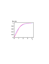
Figure 3: (Color online) Cumulative spacing momentum distributions for different regions of measured momenta: a)$0.1<|p|<1.14$ GeV/c (solid line); b)$1.14<|p|<4.0$GeV/c (dashed line); c)$4.0<|p|<7.5$ GeV/c (dot-dashed line). The solid line nearly coincides with the result for the Poisson distribution, while the dot-dashed line is close to the Wigner surmise distribution.

From the above analysis one may conclude that in this particular experiment the method enables us to reveal structural changes in the system at particular energy regions. At high energies (the third interval) the particles are produced at relatively small spatial separation, since $\Delta p$ is large and one can make use of the uncertainty relation $\Delta p\Delta x\sim\hbar$. Thus, one might expect enhanced correlations. These correlations continue to persist at the second interval but with a lesser intensity. And, finally, in the first interval the secondary particles move independently in the spatial separation defined by the kinematics. To illuminate the physical nature of this observation we consider below the method of effective mass, traditionally used to process the data produced at high energy nucleus-nucleus collisions.

To complete the discussion we calculate the integrated momentum spacing density for experimental data in order to confirm that all distributions have on average a constant mean spacing ($=1$). This is an additional test which verifies the convergence of our calculations. Fig.3 shows the integrated density, demonstrating a gradual transition from a Poisson-like density toward a Wigner-like density with the increase of the absolute value of the momentum distributions.

III Method of effective mass

In this section we consider the method of effective mass (MEM) b4 , which is a standard tool to extract the information on the correlation between secondary particles.

Before we proceed a few remarks are in order: in various theoretical approaches it is usually assumed that at high-energy nucleus-nucleus collisions: i) a majority of produced secondary pions are emitted basically through the mechanism of production and decay of the light resonances; ii) a significant portion of the protons are produced as a result of $\Delta$-isobar decays b9 . Further, it is also assumed that such processes consist of two steps. First, $(n-k)$ particles and the resonance are produced. Second, the resonance decays on $k$-particles and one may expect that due to kinematics there are some correlations between these $k$-particles. In order to extract these correlations we are forced to consider all possible combinations of the $k$-particle-participants and compare with the known resonance masses.

In particular, in the MEM one considers the effective mass for k secondary particles which create a cluster (a resonance) as

$$M_{k}=\biggl{\{}(\sum_{i=1}^{k}E_{i})^{2}-(\sum_{i=1}^{k}{\vec{p}}_{i})^{2}\biggr{\}}^{1/2}\,.$$ (8)

If the condition $M_{k}=M_{k}^{res}$ holds, one may conclude that a resonance with the mass $M_{k}^{res}$ is identified in the data. In addition, one assumes that each identified resonance contributes to the total cross section with its own weight (probability). To carry on this idea, each resonance is approximated by the Breit-Wigner distribution with the identified mass and the resonance width. Varying the weights of identified resonances, one is aiming to reach the best agreement with the observed inclusive cross sections of resonances production. This procedure proved to be reasonable at small multiplicity of the secondary particles or at relatively small energies per particle ($<10$ GeV/c). The situation changes drastically at the large multiplicity, where number of the secondary particles is more than ten in each event. For example, suppose that we have $N$ secondary particles in each event. The most favorable case is where each pair of the secondary particles creates a resonance; the number of resonances $N_{\it res}=N/2$ in the event. However, we have to consider all independent combinations between pairs in the event and, therefore, the total number of physical and ”spurious” resonances is $N_{\it tot}=N*(N-1)/2$. It results in the ratio $r=N_{\it res}/N_{\it tot}\sim 0.1$ (a ”useful” signal) for ten particles in the event. Evidently, this procedure gives rise to a large spurious contribution to the analysis.

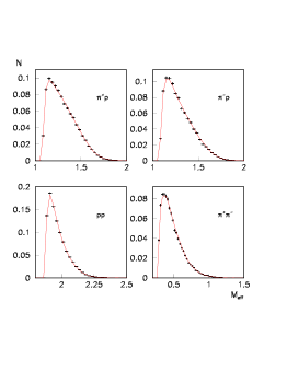
Figure 4: (Color online) The distributions (crosses) of $(\pi^{+}p)$–, $(\pi^{-}p)$–, $(pp)$–, and $(\pi^{+}\pi^{-})$–pairs emitted in the interval of the momentum distribution of the secondary particles $0.1<|p|<1.14$ GeV/c. The background is shown by solid line. The total number of pairs is normalized to unity.

Further, to extract the information on the resonance production from data it is necessary to evaluate a background contribution. It is indeed a difficult task which cannot be solved completely. Therefore, to construct the background the method of mixing events mme is usually used. In this method the background is defined by the pairs constructed from the particles produced in different events only. Note, that this procedure may lead to the violation of the energy and momentum law conservation due to the mixing of different events. Finally, the resonance production is associated with the existence of the difference between the distribution of all independent combinations ($N_{\it tot}=N*(N-1)/2$) in the event and the background distribution for the pairs.

Keeping this in mind, we consider the distributions of charged particle pairs emitted in ¹²C+¹²C -interactions at $4.2$ A GeV/c int3 ; [9] . Figs.4-6 demonstrate the distributions of $(\pi^{+}p)$–, $(\pi^{-}p)$–, $(pp)$–, and $(\pi^{+}\pi^{-})$–pairs emitted in three ranges of the momentum distribution of the secondary particles: $0.1-1.14$ (Fig.4); $1.14-4.0$ (Fig.5) and $4.0-7.5$ GeV/c (Fig.6). All distributions are normalized to the total number of pairs. Note, the lowest threshold for the effective masses scale is determined by the individual mass of each participant and their momenta, according to Eq.(8).

One observes that in the interval of momentum $0.1-1.14$ GeV/c (Fig.4) no clear-cut distinction exists between experimental and background distributions. In this interval we have obtained very good statistical conditions: 41615 $(\pi^{+}p)$–, 43626 $(\pi^{-}p)$–, 52992 $(pp)$– and 39112 $(\pi^{+}\pi^{-})$–pairs. One concludes that there is no a manifestation of a resonance production. We recall that in this interval the RMT approach produces the Poisson distribution for the behavior of the $p(s)$-function (see Fig.2a). In other words, the NND indicates on the absence of any correlations in this energy interval.

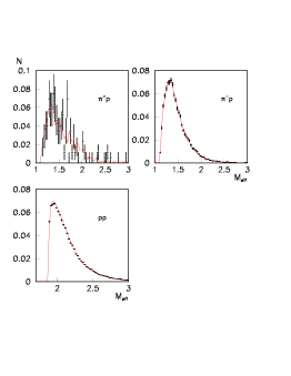
Figure 5: (Color online) Similar to Fig.4 for the interval $1.14-4.0$ GeV/c.

In the second interval (see Fig.5) we have obtained 173 $(\pi^{+}p)$–, 16470 $(\pi^{-}p)$–, 167094 $(pp)$– and only 16 $(\pi^{+}\pi^{-})$–pairs (are not shown). There is some deviation of the experimental distribution from the background only for $(\pi^{+}p)$–pairs. Although the error bars are noticeable, there is a clear indication on the resonance production at $1.1<M_{\it eff}<2$ (GeV$/c^{2}$). We believe that it is connected with the production of the $\Delta^{++}$-isobars with masses $m_{\Delta^{++}}=1.232$ and $1.650$ (GeV$/c^{2}$). Note that the observation of $\Delta^{++}$-isobars with masses $m_{\Delta^{++}}=1.232$ GeV$/c^{2}$ has been reported in b9 , while the ones with masses $1.650$ GeV$/c^{2}$ are observed for the first time in the present data. The statistics are not enough, however, to support strongly the latter observation. There are no visible deviations between the experimental data and the background for the distribution of the $(\pi^{-}p)$– and $(pp)$–pairs. In this interval the RMT approach produces a visible deviation from the Poisson distribution for the behavior of $p(s)$-function (see Fig.2c), i.e., the NND signals upon the onset of correlations. The agreement between predictions obtained in two different approaches confirms that the NND is able to provide a hint of the resonance production.

In the third interval of the momentum distribution of charged secondary particles we have 10 $(\pi^{-}p)$– (are not shown) and 9522 $(pp)$–pairs (Fig.6). Here, the $(\pi^{+}p)$–pairs are absent. One observes a clear cut distinction between the background and experimental distribution of $(pp)$–pairs in $4.0-7.5$ GeV/c. The deviation of the signal relative to the background is above $20\%$. However, there is no a solid basis to associate such a strong deviation with a production of di-baryon resonances debar , since the inclusive cross section of such ”resonances” would exceed essentially those that are predicted by various theoretical models.

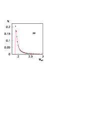
Figure 6: (Color online) Similar to Fig.4 for $(pp)$–pairs emitted in the interval of the momentum distribution of the secondary particles $4.0-7.5$ GeV/c.

It is well known that in this interval the stripping protons are the dominant ones (with a small contribution of deuterons, tritons and others) int3 . These protons carry a maximum momentum near the value 4.2 GeV/c. It results in very small deviations of the particle trajectories in the magnetic field of the setup. In fact, it is the worst situation for the accurate determination of the errors in the momentum distribution. The RMT approach produces in this interval a distribution of the density $p(s)$ close to the Wigner surmise form (see Fig.2e). As stressed above, such a distribution is associated with the breaking of regularity in the spectral properties of a quantum system due to either external or internal sources. In sh1 we have already mentioned that the onset of the Wigner distribution for the density $p(s)$ (breaking of the regularity) could indicate the presence of errors in the measurements, i.e., the correlations introduced by external perturbations.

Figure 7: Left: The proton distributions $dN/d|p|$ as a function of the measured momentum in three different regions: $0.1-1.14$ (a); $1.14-4.0$ (c) and $4.0-7.5$ (e) (GeV/c). Right: The proton distributions $dN/d\theta$ as a function of the angle in three different regions: $0.1-1.14$ (b); $1.14-4.0$ (d) and $4.0-7.5$ (f) (GeV/c). The angular distribution is normalized to unity.

To gain a better insight into the nature of correlations, it is worthy of note that in all considered distributions there is an evident dominance of the $pp$-pairs. To trace the evolution of the $pp$ correlations we select only the momentum and angular distributions of the protons in three intervals (see Fig.7). In the first interval the angular distribution (see Fig.7b) of the pairs covers almost all angles of the semisphere with some concentration around $\sim 50^{0}$. We recall that the NND (see Fig.2b) displays the Poisson distribution in this region, which is typical for a noninteracting system. The absence of the correlations for lower-energy proton pairs is due to Fermi protons (with the average momentum $\sim 300$ MeV/c) which move as independent particles. The angular distribution is determined by the kinematics (the momentum and the energy conservation laws). In the second interval the momentum distribution of the pairs (Fig.7c) is spread smoothly over all considered values of the momentum ($1.14-4.0$ GeV/c). There is some concentration of the emitted pairs in the angular distribution, which covers a solid angle $\sim 20^{0}$ (Fig.7d). The protons can be divided on participants and spectators. The participants are due to the $\Delta$-isobar and excited nucleon decay, and also consist of the protons which acquire momenta in direct nuclear reactions. Although there are some signature of spectators, they are dominant in the third region. For the second region we obtain the NND pattern which is neither the Poisson nor the Wigner type (Fig.2d). In the third interval (Figs.7e,f) one observes that stripping protons have similar momenta and almost zero angle in the distribution. Evidently, under such conditions, one may expect a large probability for the interaction in the final state, which leads to the narrow peak appearances in the effective mass spectrum of the proton pairs. Such interaction effects in a final state are well known for the particle production and decay process at high energies fin . We recall that for this interval the RMT approach provides the Wigner distribution (Fig.2f) for the behavior of the density $p(s)$. In other words, the NND indicates that in this region there are strong correlations that break the regularity in the spectra. The maximum of the correlation is observed to increase with the increasing of the kinetic energy. This may indicate that the energetic protons create clusters due to strong pairing effects at short time intervals. We will return to this point in the next section.

The comparison of the NNDs with the MEM analysis manifests in fact that there are evident correlations between behavior of the density $p(s)$ in different energy (momentum) intervals and the appearance of new sources that break the regularity in the momentum distribution of the charged particles. The NNDs discussed in the previous section indicate the onset of correlations (a production of resonances) at the intermediate region unambiguously, via the deviation of the spacing distribution from the Poisson limit (see Fig.2). According to the MEM analysis the stripping protons are responsible for the strong correlations in the third interval. We stress that the presence of strong correlations is predicted independently by the NND which exhibits the Wigner distribution in this region. Presently, however, we cannot distinguish between correlations introduced by the physical process and by possible errors in the measurements. This is one of the main challenges for the RMT approach in high energy physics.

IV Correlations

In order to characterize the degree of correlations for a stationary spectrum with unit average spacing Dyson introduced the k-level correlation functions

$$R_{k}(x_{1},...,x_{k})=\frac{N!}{(N-k)!}\int...\int P_{k}(x_{1},...,x_{N})dx_{k+1}...dx_{N}$$

$$1\leq k\leq N,$$ (9)

where $P_{N}(x_{1},...,x_{N})dx_{1}...dx_{N}$ gives the probability of having one eigenvalue at $x_{1}$, another at $x_{2}$…, another at $x_{N}$ each within the interval $\{x_{i},x_{i}+dx_{i}\}$. By integrating $P_{k}(x_{1},...,x_{N})$ over all variables but one, in the limit $N\rightarrow\infty$, one obtains the ensemble averaged density

$$\tilde{\rho}(x_{1})=\int...\int P_{k}(x_{1},...,x_{N})dx_{2}...dx_{N}\,,$$ (10)

which is normalized to unity. From Eq.(9) it follows that $R_{1}(x_{1})=N\tilde{\rho}(x_{1})$ and $R_{k}(x_{1},...,x_{k})dx_{1}....dx_{k}$ is the probability, irrespective of the index, of finding one level within of each of the intervals $[x_{i},x_{i}+ds]$. From the above definition it follows that $R_{1}(x)=1$. With the aid of the definition (9), by integrating $R_{k+1}$ one obtains

$$\int R_{k+1}(x_{1},...,x_{k+1})dx_{k+1}=(N-k)R_{k}(x_{1},...,x_{k})\;.$$ (11)

Figure 8: (Color online) Number variance $\Sigma^{2}(L)$ for three different regions of the experimental spacing momentum distributions: a)$0.1<|p|<1.14$ GeV/c (solid line); b)$1.14<|p|<4.0$GeV/c (dashed line); c)$4.0<|p|<7.5$ GeV/c (dot-dashed line).

It is difficult to work directly with the $R_{k}$ functions. One important and more convenient measure of correlation that was introduced is based on the number statistic $n(E,L)$ which is defined to be the number of levels in an energy interval of length $L$ and centered at the energy (momentum) $E$:

$$n(E,L)=\int_{E-L/2}^{E+L/2}\rho(E)dE\,.$$ (12)

Since the spectrum was unfolded (see Eq.(5)), the ensemble average number statistic $\langle n(E,L)\rangle=L$ is independent of the spectrum. However, the variance of $n(E,L)$

$$\Sigma^{2}(L)=\langle[n(E,L)-\langle n(E,L)\rangle]^{2}\rangle,$$ (13)

does depend on the spectrum considered. For the Poisson density (see meh )

$$\Sigma^{2}(L)=L,$$ (14)

and for the GOE one the exact asymptotic expression is

$$\Sigma^{2}(L)=\frac{2}{\pi^{2}}\Bigg{[}ln(2\pi L)+\gamma+1+\frac{1}{2}[Si(\pi L)]^{2}-\frac{\pi}{2}Si(\pi L)$$

$$-\cos(2\pi L)-Ci(2\pi L)+\pi^{2}L\left[1-\frac{2}{\pi}Si(2\pi L)\right]\Bigg{]}\,.$$ (15)

Here $\gamma$ is the Euler constant and $Si$, $Ci$ are the sine and cosine integrals, respectively. The number variance $\Sigma^{2}(L)$ calculated using the optimal implementation of the definition in Eq.(13) is shown in Fig. 8. Indeed, this quantity manifests the Poisson statistics (Eq.(14)) for experimental spectra with a low momentum distribution. On the other hand, one again observes a clear indication of the presence of correlations for large momenta.

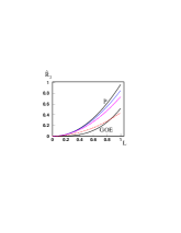
Figure 9: (Color online) Two-point correlation function ${\hat{R}_{2}}(s=L)$ for different regions of measured momenta: a)$0.1<|p|<1.14$ GeV/c (solid line); b)$1.14<|p|<4.0$GeV/c (dashed line); c)$4.0<|p|<7.5$ GeV/c (dot-dashed line). The solid lines, denoted as P and GOE, display the characteristic limits for Poisson and GOE ensembles, respectively.

For the analysis of fluctuations it is more convenient to use pure k-point functions BHP

$$\hat{R}_{k}(L)=\int_{0}^{L}...\int_{0}^{L}R_{k}(x_{1},...,x_{k})dx_{1}...dx_{k}\,.$$ (16)

The function $\hat{R}_{k}(L)/k!$ gives the probability that an interval of length $L$ (for small $L$) contains $k$ levels. In the RMT most emphasis has been put on the two-point correlation function ${\hat{R}_{2}}(x_{1},x_{2})$ or density-density correlation function. The two-point correlation function is the probability density to find two eigenvalues $x_{i}$ and $x_{j}$ at two given energies (momenta), irrespective of the position of all other eigenvalues. The function $R_{2}(x_{1},x_{2})$ depends only on the relative variables $s=x_{1}-x_{2}$ defined in Sec.II. The variance $\Sigma^{2}$ is connected to $\hat{R}_{2}$ through the following relation

$$\hat{R}_{2}(L)= \int_{0}^{L}\int_{0}^{L}R_{2}(x_{1},x_{2})dx_{1}dx_{2}-2\int_{0}^{L}(L-s)R_{2}(s)ds$$

$$= \Sigma^{2}(L)+L(L-1)\,.$$ (17)

The two-level correlation function $R_{2}(x_{1},x_{2})$ determines the basic fluctuation measures related to Wigner’s level repulsion and the Dyson-Mehta long-range order, i.e., large correlations between distant levels. Bohigas et al BHP provided a thorough analysis of level repulsion and long-range correlations (rigidity) for different correlation functions. To understand the distinct role played by level repulsion and long-range order in the momentum density, we compare our numerical results with analytical expressions from Table 1 of Ref.BHP, for the Poisson ensembles (there is neither level repulsion nor long-range order) and for the GOE case (this ensemble exhibits both features). The two-point correlation function ${\hat{R}_{2}}(x_{1},x_{2})$ calculated from Eq.(17) is shown in Fig.9. Even though there are small deviations from the Poisson $(\hat{R}_{2}(L)=L^{2})$ and the GOE $(\hat{R}_{2}(L)=\pi^{2}L^{3}/18)$ predictions, the experimental results for the momentum distributions reproduce surprisingly well both limits.

We recall that the analysis is based on the unfolded spectra obtained from the experimental momentum distribution (Sec.II). In contrast to the MEM, the above procedure does not introduce any ”spurious” correlations due to combinatorics. In addition, each event is treated separately. However, the two-point correlation function ${\hat{R}_{2}}(x_{1},x_{2})$ clearly exhibits the presence of correlations in the experimental data. It is another beautiful example how the correlations can show up in the Dyson-Mehta statistics. Thus, the transition from the Poisson limit to the GOE implies the onset of strong correlations at the region III.

As was stressed above the two-point correlation function ${\hat{R}_{2}}(s=L)$ indicates upon large correlations between distant levels (momentum). It appears that the transition to the GOE limit might signal on the formation of clusters. These clusters should consist of energetic protons mainly, which seems move pairwise in the third interval (see Fig.7f). Note, however, that the NNDs for the third region indicate on the Wigner repulsion. The physical nature of this phenomenon may be understood with the aid of the Hanbury-Brown-Twiss (HBT) analysis of the proton correlations boal . The HBT analysis focuses on the spatial distribution of the radiation area, being very sensitive, however, to the statistical assumptions upon the background distribution. Evidently, such analysis represents a separate problem itself and is beyond the scope of the present paper.

Nevertheless, it is interesting to note, that the standard pair-correlation function (see, for example, Ref.gol, and references therein)

$$R(y_{1},y_{2})=\sigma\frac{d^{2}\sigma/dy_{1}dy_{2}}{(d\sigma/dy_{1})(d\sigma/dy_{2})}-1,$$ (18)

used for the analysis of data in high-energy physics, might be useful to compare with the RMT results. Here, the quantity $\sigma$ is the cross section of the inclusive reaction and $y=\frac{1}{2}ln\frac{E+P_{||}}{E-P_{||}}$ is the rapidity, which depends on the particle energy $E$ and its longitudinal momentum $P_{||}$. The rapidity is one of the main characteristics widely used in relativistic nuclear physics (see b2 ; b4 ). In particular, the change of the reference frame leads to a trivial shift $\Delta y$ in the rapidity. The pair-correlation function manifests the difference between the probability density of two-particle events and the product of the probability densities of independent particle events. It vanishes if the particle rapidities are independent, i.e., the correlations are absent. In a way, this function is similar in spirit to the two-point correlation function ${\hat{R}_{2}}(x_{1},x_{2})$, or density-density correlation function of the RMT. Therefore, it is useful to compare the predictions obtained by dint of the RMT tools and with the aid of the standard pair-correlation function.

Figure 10: Integrated two-pair correlation functions for particles obtained in ¹²C+¹²C-interactions (see the text) for different regions of measured momenta: a)$0.1<|p|<1.14$ GeV/c; b)$1.14<|p|<4.0$GeV/c; c)$4.0<|p|<7.5$ GeV/c.

Fig.10 displays results for the standard pair-correlation function, obtained for ¹²C+¹²C-interactions. The function $R(y_{1},y_{2})$ was integrated over one of the variables, say $y_{1}$, and we consider the dependence of this function on $y_{2}$. For different momentum distributions, there are three intervals of integration for the variable $y_{1}$: a)for $0.1<|p|<1.14$ GeV/c the function $R(y_{1},y_{2})$ is integrated in the interval $-1.0<y_{1}<2.5$; b)for $1.14<|p|<4.0$ GeV/c it is integrated in the interval $0.1<y_{1}<2.4$; and c)for $4.0<|p|<7.5$ GeV/c it is integrated in the interval $2.5<y_{1}<3.5$. The results for the function $R=\int_{y_{1}}R(y_{1},y_{2})dy_{1}$ clearly indicate the presence of correlations between particles in the region $4.0<|p|<7.5$ GeV/c : there is a strong deviation from zero in the interval $2.7<y_{2}<3.2$. While this function does not exhibit any signature of correlation in the second region, one observes a strong correlations between rapidities in the third region. We recall that in this interval the NND exhibits the Wigner distribution (short-range correllations), typical for strongly correlated system. Thus, we speculate that in the region III there is a formation of the short-living proton pairs (see also Sec.III).

V Summary

Using the Dyson-Mehta statistical measures for the first time for analysis of data in high energy physics, we have studied the experimental data from ¹²C+¹²C collisions at 4.2 A GeV/c. The high accuracy of the data provides a reliable basis for the analysis of the momentum distribution of the secondary charged particles produced in this reaction. The NND analysis (Sec.II) indicates on the onset of correlations in the momentum distribution interval $1.14<|p|<4.0$ GeV/c (region II). The results of calculations for different correlations functions (Secs.II,IV) evidently demonstrate the presence of strong correlations in the momentum distribution interval $4.0<|p|<7.5$ GeV/c (region III).

We have analysed the same data with the aid of the method of effective mass, one of the standard tools for analysis of data produced at nucleus-nucleus collisions at high energies (see Sec.III). The results of this analysis exhibits the presence of strong correlations, independently found by dint of the RMT approach. In the region II we found the production of well known $\Delta^{++}$-isobars with masses $m_{\Delta^{++}}=1.232$ and $1.650$ (GeV$/c^{2}$). The dominance of the proton pairs with zero angle in the momentum distribution interval $4.0<|p|<7.5$ GeV/c could be attributed to the interaction effects in the final state. It appears that these effects may lead to the formation of the short-living proton pairs. Note that the method of effective mass involves, however, some additional assumptions that induce unavoidable uncertainty in the analysis due to a large nonphysical contribution to the data. This may cause additional errors, which are difficult to exclude with the aid of the approaches widely used for the analysis of nucleus-nucleus collisions at high energies. In contrast, the RMT approach is independent of such spurious contributions. The only requirement of the RMT is that the local mean densities (or secular behaviors) should be understood and their effects removed through the use of the unfolding procedure (see Sec.II), which is a routine procedure for the RMT. By dint of relatively simple and transparent mathematical tools, the RMT approach detects the appearance of new sources that break the regularity in the momentum distribution.

Furthermore, the predictions based on the RMT analysis are consistent with the predictions based on the standard pair-correlation function $R$ (see Sec.IV), which is another tool for the analysis of data produced at nucleus-nucleus collisions at high energies. In fact, the RMT two-point correlation function magnifies the presence of correlations manifested in the standard pair-correlation function (compare Figs.9 and 10c). We stress that the uncertainty of the results encountered in the theoretical analyses of the multiplicity fluctuations in different statistical ensembles beg does not appear in the RMT approach at all. The Dyson-Mehta statistical measures rely heavily on the fundamental symmetries preserved in the nucleus-nucleus collisions.

We conclude that the RMT approach is free from various assumptions concerning the background of the measurements and it provides reliable information about correlations induced by external or internal perturbations. We recall that it is expected that at central heavy-ion collisions at relativistic energies the multiplicity of secondary particles will increase drastically. Evidently, the standard tools like the MEM approach (Sec.III) would encounter a large uncertainty due to the increase of spurious background contributions in the analysis of data. In contrast, the efficiency of the RMT approach increases with the increase of the multiplicity of the secondary particles in each event taken individually. We stress that the RMT approach is based on a unique, mathematically rigorous theory at the limit of $N\rightarrow\infty$. Therefore, we believe that our analysis provides the basis for further development of quantitative methods based on the ideas of the RMT for data processing produced at nucleus-nucleus collisions at high energies.

References

- (1) H. Heiselberg, Phys. Rep. 351, 161 (2001).
- (2) S. Jeon and V. Koch Review for Quark-Gluon Plasma 3 Eds. R. C. Hwa and X.-N. Wang (World Scientific, Singapore, 2004) pp 430-490.
- (3) E. A. De Wolf , I. M. Dremin, and W. Kittel, Usp. Fiz. Nauk 163, 3 (1993) [Phys. Usp. 36, 225 (1993)].
- (4) E. Byckling and K. Kajantie, Particle Kinematics (Wiley, New York, 1973).
- (5) V. I. Gol’danckiy, Yu. P. Nikitin, and I. L. Rozental’, Kinematic methods in high energy physics ( Nauka, Moscow, 1987) (in Russian).
- (6) M. I. Podgoretsky, Fiz. Elem. Chastits At.Yadra, 20, 628 (1989).
- (7) M. Gazdzicki, M. I. Gorenstein, and S. Mrowczynski, Phys. Lett. B 585, 115 (2004).
- (8) J. Cleymans, H. Oeschler, K. Redlich, and S. Wheaton, Phys. Rev. C 73, 034905 (2006).
- (9) F. Becattini, J. Manninen, and M. Gazdzicki, Phys. Rev. C 73, 044905 (2006).
- (10) A. Andronic, P. Braun-Munzinger, and J. Stachel, Nucl. Phys. A 772, 167 (2006).
- (11) V. V. Begun, M. Gazdzicki, M. I. Gorenstein, and O. S. Zozulya, Phys. Rev. C 70, 034901 (2004).
- (12) S. A. Bass et al., Prog. Part. Nucl. Phys. 41, 255 (1998).
- (13) B. Borderie and M. F. Rivet, Prog. Part. Nucl. Phys. 61, 551 (2008).
- (14) M. L. Mehta, Random Matrices (Elsevier, Amsterdam, 2004) Third Edition.
- (15) C. E. Porter, Statistical Theories of Spectra: Fluctuations (New York: Academic, New York, 1965).
- (16) T. A. Brody, J. Flores, J. B. French, P. A. Mello, A. Pandey, and S. S. M. Wong, Rev. Mod. Phys. 53, 385 (1981).
- (17) E. P. Wigner, Ann. Math. 53, 36 (1951); reprinted in Porter’s book above.
- (18) T. Cuhr, A. Müller-Groeling, and H. Weidenmüller, Phys. Rep. 299, 189 (1998).
- (19) E. I. Shahaliev, R. G. Nazmitdinov, A. A. Kuznetsov, M. K. Syleimanov, and O. V. Teryaev, Physics of Atomic Nuclei 69, 142 (2006).
- (20) O. Balea et al., (BBCDHSSTTU-BW Collaboration) Phys. Lett. B 39, 571 (1972).
- (21) N. Akhababian et al., JINR Report, No. 1-12114, Dubna (1979).
- (22) D. D. Armutliiski et al., (BBCDHSSTTU-BW Collaboration), Yad. Fiz. 45, 1047 (1987).
- (23) H. N. Agakishiyev et al., Zeit. für Physik C - Particles and Fields 27, 177 (1985).
- (24) A. Bondarenko et al., JINR Rapid Communications, P1-98-292, Dubna (1998).
- (25) O. Bohigas, Lecture Notes in Physics 263 (Springer-Verlag, Berlin, 1986) p.18.
- (26) O. Bohigas, M. J. Giannoni, and C. Schmit, Phys. Rev. Lett. 52, 1 (1984).
- (27) W. D. Heiss, R. G. Nazmitdinov, and S. Radu, Phys. Rev. Lett. 72, 2351 (1994); Phys. Rev. C 52, 3032 (1995).
- (28) V. G. Grishin, et al., JINR Report, P1-88-821, Dubna (1988).
- (29) G. I. Kopylov, Phys. Lett. B 50, 472 (1974).
- (30) L. S. Vorobev et al., Yad. Fiz. 51, 135 (1987).
- (31) R. Lednicky and V. L. Lyuboshitz, JINR Communication, P2-92-546, Dubna (1992).
- (32) O. Bohigas, R. U. Haq, and A. Pandey, Phys. Rev. Lett. 54, 1645 (1985).
- (33) D. H. Boal, C.-K. Gelbke, and B. K. Jennings, Rev. Mod, Phys. 62, 553 (1990).
- (34) A. I. Golokhvastov, Physics of Atomic Nuclei 67, 2227 (2004).