Interaction of Close-in Planets with the Magnetosphere of their Host Stars I: Diffusion, Ohmic Dissipation of Time Dependent Field, Planetary Inflation, and Mass Loss

Abstract

The unanticipated discovery of the first close-in planet around 51 Peg has rekindled the notion that shortly after their formation outside the snow line, some planets may have migrated to the proximity of their host stars because of their tidal interaction with their nascent disks. After a decade of discoveries, nearly 20 % of the 200 known planets have similar short periods. If these planets indeed migrated to their present-day location, their survival would require a halting mechanism in the proximity of their host stars. Here we consider the possibility that a magnetic coupling between young stars and planets could quench the planet’s orbital evolution. Most T Tauri stars have magnetic fields of several thousand gausses on their surface which can clear out a cavity in the innermost regions of their circumstellar disks and impose magnetic induction on the nearby young planets. After a brief discussion of the complexity of the full problem, we focus our discussion on evaluating the permeation and ohmic dissipation of the time dependent component of the stellar magnetic field in the planet’s interior. Adopting a model first introduced by Campbell for interacting binary stars, we determine the modulation of the planetary response to the tilted magnetic field of a non-synchronously spinning star. We first compute the conductivity in the young planets, which indicates that the stellar field can penetrate well into the planet’s envelope in a synodic period. For various orbital configurations, we show that the energy dissipation rate inside the planet is sufficient to induce short-period planets to inflate. This process results in mass loss via Roche lobe overflow and in the halting of the planet’s orbital migration.

.

1 Introduction

Perhaps the most surprising finding in the search for extrasolar planets is the discovery of short-period ($P<1$ week) Jupiter-mass ($M_{J}$) companions around Solar-type main sequence stars (Mayor & Queloz 1995, Marcy et al. 2000). Among the inventory of $>$200 presently-known extrasolar planets, 20% have $P=1-7$ days. Nearly 20 short-period planets have measured radii ($R_{p}$) that are comparable to or larger than that of Jupiter ($R_{J}$). While these information may be biazed because of observational selection effects, these planets are most probably gas giants.

According to the conventional sequential-accretion scenario (Pollack et al. 1996), the most likely birth place for gas giant planets is just outside the snow line where volatile heavy elements can condense and coagulate into large planet building blocks (Ida & Lin 2004). In protostellar disks with comparable surface density ($\Sigma$), metallicity ([Fe/H]), and temperature ($T$) distributions as those of minimum mass nebula model (Hayashi et al. 1985), protoplanets with $M_{p}\sim M_{J}$ induce the formation of a gap near their orbit as a consequence of their tidal torque on the nascent disks (Goldreich & Tremaine 1978, 1980, Lin & Papaloizou 1980, 1986a, 1993). In relatively massive and fast evolving disks, the outward transfer of angular momentum due to the disks’ intrinsic turbulence can lead to an inward mass flux ($\dot{M}_{d}$) and the migration of the gas giant planets (Lin & Papaloizou 1986b). This process is commonly referred to as type II migration (Ward 1997).

This migration scenario was resurrected to account for the origin of the first known short-period extra solar planet (Lin et al. 1996). Although type-II migration provides a natural avenue for relocating some gas giants, a mechanism is needed to retain these planets close to their host stars. Moreover, many stars are born with rapid rotation (Stassun 2001). When young planets venture close to their host stars, angular momentum would be transferred from the stellar spin to the planet’s orbit if the stellar spin frequency $\omega_{\ast}$ is still larger than the planet’s orbital frequency ($\Omega_{k}$). The rate of the star-to-planet angular momentum transfer intensifies rapidly and may exceed that from the planet to the disk.

Two basic physical effects were suggested as potential migration barriers. The first one is tidal interaction between the host star and the planet. The gravitational perturbation of the star and close-in planet leads to responses in both the star and planet. For tidal frequencies smaller than twice the spin frequency, inertial waves are excited in the convective envelope of the host star and are dissipated there by turbulent viscosity (Ogilvie & Lin 2007). But, the tide excited by a close-in gas giant planet in a star, with a structure similar to that of the present Sun, marginally fails to achieve nonlinearity so that their survival is ensured. Nevertheless, during the formation epoch of solar-type stars, conditions at the center of the star evolve, so that nonlinearity may set in at a critical age, resulting in a relatively intense star-planet tidal interaction.

The second effect suggested is based on the magnetic interaction between the host star and the planet. Young T Tauri stars also have radii ($R_{\ast}$) 2-3 times that of the present-day Sun ($R_{\odot}$) and several thousand gausses fields ($B_{\ast}$) on their surface (Johns-Krull 2007). The stellar magnetosphere threads across the inner regions of the disk and clears a cavity out to a critical radius ($R_{c}$) which is determined by both the magnitude $B_{\ast}$ and $\dot{M}_{d}$ (Konigl 1991). The subsequent complex interplay between accretion and outflow leads to angular momentum exchange which induces $\omega_{\ast}$ to evolve toward $\Omega_{k}$ at $R_{c}$ (Shu 1994). When the planet’s orbital semi major axis ($a$) reduces well inside $R_{c}$, its Lindblad resonances relocate inside the star’s magnetospheric cavity. In principle, the planet’s migration would stall due to its diminishing tidal torque on the disk.

However, if the star’s magnetospheric interaction with the disk can lead to $\omega_{\ast}=\Omega_{k}(R_{c})$, the planet inside the magnetospheric cavity would have $\Omega_{k}>\omega_{\ast}$. In this limit, the star-planet tidal interaction would induce a transfer of angular momentum from the planet to the star. In addition, the differential motion between the planet and the stellar spinning magnetosphere induces an electromagnetic field with a potential to generate a large current analogeous to the interaction between the Jovian magnetosphere with its satellite Io (Goldreich & Lynden-Bell 1969). The associated Lorentz force drives an orbital evolution toward a synchroneous state, in which case, angular momentum would be transferred from the planets with $\Omega_{k}>\omega_{\ast}$ to their host stars, and the planets would continue their orbital decay.

In order to determine the necessary condition for the retention of close-in young planets, we examine, in this paper, their interaction with the magnetosphere of their host T Tauri stars. In §2, we briefly recapitulate the essential concepts and validity of previous investigations on some related topics and give an overview of the key phenomena that will be discussed in this and later papers. In §3, we adopt an existing model in order to examine the interaction between a planet and the magnetosphere of its host star. In §4, we compute precisely the planet’s magnetic diffusivity for a specific set of parameters, as well as the corresponding ohmic dissipation rate within that planet. In §5, we suggest that the ohmic dissipation can generate sufficient heat to inflat the planet. In §6, we construct an idealized self-consistent model in which the polytropic and isothermal equations of state are utilized. These equations represent the expected outcome of radiation transfer within the fully convective interior and the isothermal surface of a close-in planet which is exposed to the intense radiation from its host star. This internal model allows us to compute the magnetic diffusivity. With these tools, we discuss in §7 the structural adjustment of the planet in response to this heating source and we compute the ohmic dissipation and mass loss rate for different set of parameters. Finally in §8, we summarize our results and discuss their implications.

2 Planetary and astrophysical analogue

Two previous analyses are directly relevant to the present study: 1) the interaction of Io with the magnetosphere of Jupiter and 2) the spin-orbit synchronization in binary stars containing a magnetized white dwarf and its main sequence or white dwarf or planetary companion.

2.1 Unipolar Induction in Io

Io orbits around Jupiter inside its magnetosphere once every 1.7 days which is considerably longer than Jupiter’s 10 hours spin period. This relative motion imposes a periodic variation in Jupiter’s decametric emission (Duncan 1966). A class of models that accounts for the origin of this emission was developped based on the assumption that Io has a sufficiently high conductivity. In Io’s rest frame, the electric field vanishes and the steady component of Jupiter’s magnetic field permeates in Io’s interior over time. When a steady state is established, the tube of constant magnetic flux is firmly frozen into Io (Piddington and Drake 1968) due to its high conductivity. The flux tube carried by Io moves through the surrounding field lines (which corotate with Jupiter) and slips through Jupiter’s less conductive ionosopheric surface. Plasma in Jupiter’s ionosphere flows around the tube and introduces a potential difference across it (Goldreich & Lynden-Bell 1969). The associated electric field drives a current which travels down one half of the flux tube from Io and is sent back to Io along the other half. Within the flux tube connecting Io and Jupiter’s ionosphere and those across it on Io, the electric field vanishes as a consequence of high conductivity. Thus, this DC circuit is closed by Io as a unipolar inductor.

The magnitude of the electric current is primarily determined by the Pederson conductivity at the foot of the flux tube i.e. on the ionosphere of Jupiter. Finite conductivity also determines the magnitude of the drag against the slipage of the flux tube through Jupiter. This drag results in energy dissipation on the surface of Jupiter and in a torque on the orbital motion of Io, driving the system towards a state of synchronization. This configuration is justified by the assumption that a constant flux tube is firmly anchored on and dragged along by Io which requires the conductivity in Io to be much higher than that in Jupiter’s ionosphere. A 10^o inclination between Jupiter’s magnetic dipole and rotation axis does introduce a periodic variation (over a synodic period) in the field felt by Io. The permeation and dissipation of this time-dependent AC field may be negligible in the limit of high conductivity in Io.

The validity of the key assumption for the unipolar induction model (i.e. conductivity on Io is larger than that in Jupiter’s ionosphere) has also been challenged by Dermott (1970). A modest resistence in Io would distort the field which may lead to field slippage through Io. In this case, the passage of Io through the magnetosphere of Jupiter would lead to the generation of Alfven waves along the flux tube (Drell et al. 1965, Neubauer 1980). But, due to the field displacement, the waves, partially reflected at the foot of the flux tube on Jupiter’s surface, may not be able to return to Io, in which case the DC circuit would be broken and the motion of Io would be decoupled from the that of the flux tube. Nevertheless, the Alfven waves are dissipated inside both Io and Jupiter, leading to a torque which must depend on their penetration depth.

An alternative class of scenarios has been proposed based on the assumption that the magnetosphere is everywhere anchored on Jupiter and the flux tube moves freely through Io (Gurnett 1972). This model requires the conductivity in Jupiter’s ionosphere to be larger than that in Io. It assumes that the presence of Io creates a plasma sheath with an electric field to cancel the induced EMF associated with the motion of Io relative to Jupiter’s magnetosphere (Shawhan 1976). The simplifying approximations in the development of this theory have been challenged by Piddington (1977) who questioned both the validity of the sheath-creation mechanism and the self-consistency of the internal and external field configurations, subjected to the electric currents in and around Io.

On the observational side, UV emissions from Io’s footprint on Jupiter has been observed. But, it extends well beyond the intersection between Io’s flux tube and Jupiter’s ionosphere and the emssion downstream is protracted (Clarke et al. 1996). These observations do not agree with the simple interpretation of either the unipolar induction or the plasma sheath scenarios.

2.2 Magnetic Coupling in Interacting Binary Stars

There are many close binary-star systems with a white dwarf as their primary component. These systems also contain main sequence stars and other white dwarfs as secondary components in compact and circular orbits around each other. In some cases, mass is transferred from the secondary to the primary. In other cases, gravitational radiation may play an important role in determining the evolution of these systems.

A sub class of such interacting binary stars, AM Her systems, is composed of a magnetized white-dwarf primary and a lower-mass main sequence star as its secondary in a fully synchroneous orbit despite the ongoing mass transfer between them (Warner 1995). This orbital configuration is very similar to that of the Jupiter-Io system despite the enormous difference between the mass ratio in the two cases. The motivation for studying the impact of magnetic coupling between these stellar components is to assess whether this synchronous state can be achieved through the ohmic dissipation of the white dwarf’s field in the main sequence star’s surface (Joss et al. 1979). Toward this goal, Campbell (1983, hereafter C83) adopted a novel approach by considering the penetration and dissipation of a periodically variable field, associated with an asynchronously spinning primary.

Campbell’s approach is fundamentally different from that of the unipolar induction model. In this analysis, Campbell focussed on the flow in the envelope of the secondary and neglected the possibility of current flowing through the flux tube between the secondary star/satellite and the surface of the primary star/planet. This vacuum-surrounding approximation is justifiable since conductivity on the primary is likely to be much larger than that on the secondary and the stationary component of the field is frozen in the white-dwarf primary but not in the main-sequence secondary. Campbell analyzed the time dependent response of the secondary, including the modification of the field by the induced (AC) current in it (Campbell 2005), to the periodic modulation of the field. In contrast, the unipolar induction model depends on the explicit assumption that the field is anchored on the secondary and its distortion near the secondary must be small so that a complete current loop can be established between the primary and the secondary. Campbell determined the periodic diffusion of the field and the ohmic dissipation of the induced AC current in the companion whereas that of the induced DC current is assumed to occur in the primary in the unipolar induction model.

In recent applications of the unipolar induction model in the context of interaction between white dwarf binary stars, the current induced by the unperturbed field has been computed but the induced field generated by the current was neglected (Wu et al. 2002, Dall’Osso et al. 2006). A tidal torque is computed at the footprint of the flux tube, which is attached to the secondary white dwarf, on the surface of the magnetized primary white dwarf. A totally self-consistent solution of this diffult and complex problem remains outstanding. In addition to the uncertain anchorage location of the field, it is not clear whether the resulting misalignment of the total (original plus induced) field and current may be sufficiently large to break the circuit, in which case, Campbell’s model may be more appropriate.

2.3 Mathematical approximations made by the two previous models

In this subsection, we summarize the physical description of the two models just presented (the unipolar inductor versus the periodic diffusion) by explicating the mathematical approximations made in each one of them. The complete MHD induction equation can be expressed as

$$\frac{\partial\textbf{B}}{\partial t}=\nabla\wedge(\upsilon\wedge\textbf{B})-\nabla\wedge(\eta\nabla\wedge\textbf{B})$$ (1)

where the magnetic diffusivity $\eta=1/\mu_{0}\sigma$ and the electrical conductivity $\sigma$ functions of position and $\mu_{0}$ is the permeability. If $\eta$ is constant, the second term on the right hand side becomes $-\nabla\wedge(\eta\nabla\wedge\textbf{B})=\eta\ \nabla^{2}\textbf{B}$ which reduces to a common expression of diffusion. The two models (unipolar induction versus periodic diffusion) consider two complementary approximations of equation 1. In the problem where Io is treated as an unipolar inductor, its conductivity is explicitly assumed to be large so that the second term on the right hand (the diffusion term) is negligible compared to the first (i.e. the induction term). In this configuration, one can show that the field lines of the steady component of the magnetic field are moving with Io and appear to be ”frozen” on Io (see appendix A). Alternatively, in the model considered by Campbell, it is the first term on the right hand side that is being neglected. Moreover, only the diffusion of the time dependent component of the field is being considered. This approximation is valid if the two interacting bodies are almost in corotation (i.e. the relative speed $\upsilon$ that appears in equation (1) is small), or if the conductivity in the secondary is small.

2.4 Overview of the phenomena that will be discussed

The process under investigation in this paper is analogeous to both the Jupiter-Io and the interacting binary star problems. In fact, the unipolar induction model has already been applied to study the orbital evolution of terrestrial planets or the cores of gas giants around white dwarfs (Li et al. 1998). There are even follow-up determination of the radio flux densities from potential white-dwarf/planet systems (Willes & Wu 2005). In this analysis, although the dissipation of the induced current due to the finite conductivities in the white dwarf was considered, the feedback modification of the field and the dissipation within the planet have been neglected (Li et al. 1998). As discussed above, it is not clear whether a DC circuit can be closed to promote the unipolar induction mechanism.

In light of these uncertainties, we consider both classes of models for the interaction of close-in planets with their magnetized host stars. In this paper, we focus our discussion on the mechanism described by Campbell, and apply it to a hot-jupiter revolving around its star. We will return to the unipolar induction problem in a later paper.

When young planets first arrive at the vicinity of their host stars, they are unlikely to be in a totally synchronized state. The stellar magnetic field felt by the planet may be dominated by the periodic modulation associated with the synodic (between the stellar spin and the planet’s orbit) motion. In addition, the temperature in the planet’s surface is expected to be $\sim 10^{3}$ K and the conductivity there may be moderate. In response to the modulation of the field, the interior of the planet continually adjusts to the magnetization effects so that the flux tube cannot be effectively frozen in the planet. All of these boundary condition suggest that at least over some regions of the planet (especially on the night side where the photo ionization due to the stellar flux is negligible), the modulation of the field may lead to an induced current inside the planet which does not contribute to the close circuit of a unipolar inductor.

Following the geometry introduced by Campbell (C83), we consider a close-in gas giant planet, with a finite conductivity, interacting with a time-dependent magnetic field generated by the star. An induced current is generated inside the planet, which is associated with an ohmic dissipation rate. Our main contributions to the model used by Campbell are: 1) the relevant diffusivity inside the gas giant planets, 2) the effects of the ohmic dissipation on the planet’s internal structure, and 3) the resulting orbital evolution of the planet. (Items 2 and 3 have negligible consequence in the interacting binary star problem considered by Campbell). Since we are only considering the dissipation in the planet’s interior, the associated torque applied on its orbit should be regarded as a lower limit.

In our scenario, we postulate that at sufficiently close proximity to the host star, the stellar magnetic field is sufficiently intense that the ohmic dissipation of the periodically diffused field inside the planet is adequate to heat and to inflat the planet until it overflows its Roche lobe. The hemisphere of the planet facing its host star is also exposed to the intense flux of UV radiation during the stellar infancy. It is possible for the planet to develop a substantial ionosphere regardless the state of synchronization between the planet’s orbit and spin (the time scale for establishing local ionization equilibrium is much faster than the planet’s spin and orbital periods).

We will separately study these two phenomena (angular momentum transfert due to mass loss and presence of a ionosphere) in the follow-up papers of this serie. We will show that the angular momentum transfer associated with the mass transfer can halt the orbital evolution of the planet. We will also present an analysis on the conductivities in the planet’s day-side ionosphere and on the host stars surface. This will lead to an analysis on the condition for the unipolar induction to effectively operate and apply a significant slow-down torque on the planet’s orbit.

3 Magnetic induction

In this section, we are going to derive the governing equations that we use to compute the ohmic dissipation rate. Various equations are presented here for the purpose of introducing the algorithm of the numerical models to be presented in subsequent chapters. Although we follow closely the approach made in C83, for brevity, we do not repeatedly cite this reference. But, wherever similarities occur, referal of Campbell’s earlier work is implicitly implied. Also, throughout the paper, we use SI units.

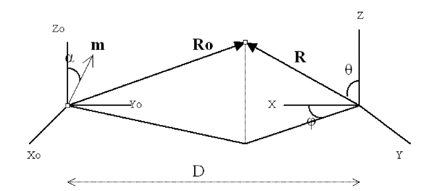
Figure 1: The geometry of the system. The star is on the left, at the center of the set of axies ($x_{0}$,$y_{0}$,$z_{0}$), and the planet is on the right, at the center of the set of axies (x,y,z).

We consider a protoplanetary system with a gas giant planet revolving around a T Tauri star with an angular frequency $\Omega_{p}$. Well beyond the planet’s semi major axis, there is also a protoplanetary disk. The host star has a dipolar moment m tilted with an angle $\alpha$ with respect to its spinning axis (see figure 1). The angular frequency of the stellar spin is $\omega_{\ast}$. The orbital axis of the disk and the planet are parallel to the star’s spinning axis. The following analysis is applied to a frame of reference centered on the star and rotating with the planet.

In this frame, the planet is a fixed object (the planet’s spin is neglected) in a periodic magnetic field with a frequency $\omega=\omega_{\ast}-\Omega_{p}$. From Ohm’s law $\textbf{J}=\sigma\textbf{E}$ and Maxwell’s equations $\frac{\partial\textbf{B}}{\partial t}=-\nabla\wedge\textbf{E}$ and $\nabla\wedge\textbf{B}=\mu_{0}\textbf{J}$, the equation on the magnetic field becomes:

$$\frac{\partial\textbf{B}}{\partial t}=-\nabla\wedge(\eta\nabla\wedge\textbf{B}).$$ (2)

It follows that in the mechanism considered by Campbell (as well as in this paper), it is the time dependent stellar magnetic field, diffusing inside the secondary (for Campbell) or the hot Jupiter (in our paper), as well as the planet’s induced magnetic field, that generate the current inside the planet, following the equation $\nabla\wedge\textbf{B}=\mu_{0}\textbf{J}$. The relative speed between the planet and the stellar magnetic field thus intervenes not through $\textbf{E}=-\upsilon\wedge\textbf{B}$ but through the time dependence in the stellar magnetic field that diffuses in the planet.

Following C83, we only consider the poloidal component $\phi$ of the magnetic field:

$$\textbf{B}\ =\ \nabla\wedge(\nabla\wedge(\phi\ \mathbf{e_{r}}))\\$$ (3)

where $\phi$ is a function of r, $\theta$, $\varphi$. and can be expanded in terms of the sperical harmonics $Y_{l}^{m}(\theta,\varphi)$ (equation 4). Moreover the variation in time of the magnetic field felt by the planet is periodic. In the limit where the field penetrates quickly in the planet compared to the time scale on which the field changes (so that the planet can respond “adiabatically”), we can account for the time dependence of $\phi$ by mutiplying its spatial part by $e^{i\omega t}$:

$$\phi(\textbf{r},t)=\mu_{0}\left[\sum_{l,m}\ C_{l}^{m}\ G_{l}(r)\ Y_{l}^{m}(\theta,\varphi)\right]e^{i\omega t}\ \ \ \ \ \ \ (l\geqslant 0\ and\ -l\leqslant m\leqslant l)$$ (4)

where $C_{l}^{m}$ are constant coefficients and $G_{l}(r)$ is a function of $r$ to be determined. We then replace B in the left hand of (2) by its expression in (3). After integration, we obtain

$$\nabla\wedge\mathbf{B}\ =-\frac{i\omega}{\eta}\nabla\wedge\left(\phi\ \mathbf{e_{r}}\right).$$ (5)

We then replace B in the left hand side of this equation using (3), and develop both sides of the equation. After identification, we obtain:

$$\frac{d^{2}G_{l}}{dr^{2}}(r)-\left(\frac{l(l+1)}{r^{2}}+\frac{i\omega}{\eta}\right)G_{l}(r)=0\ \ \ \ \ \ \ \ \ \ \ {\rm inside}\ {\rm the}\ {\rm planet.}$$ (6)

This equation holds inside and outside the planet (same as eqs 16 and 18 in C83). However, outside the planet, the conductivity is assumed to be very low and, therefore, the magnetic diffusivity is extremely high compared to the diffusivity inside the planet. In the limit where the magnetic diffusivity outside tends to infinity (equivalent to a vacuum surrounding), the equation (6) becomes:

$$\frac{d^{2}G_{l}}{dr^{2}}(r)-\left(\frac{l(l+1)}{r^{2}}\right)G_{l}(r)=0\ \ \ \ \ \ \ \ \ \ \ \ \ \ \ \ \ \ \ {\rm outside}\ {\rm the}\ {\rm planet.}$$ (7)

We consider the radial part of the poloidal scalar outside the planet. Following C83, we introduce $\phi_{star}$ the radial part of the poloidal scalar outside the planet due to the star’s magnetic field, and $\phi_{planet}$ the radial part of the poloidal scalar outside the planet due to the planet (cf C83 eqs 21-22):

$$\phi_{star}=\frac{\mu_{0}m{\rm\sin}\alpha}{8\pi d^{3}}r^{2}\left(2{\rm cos}\varphi\ {\rm\sin}\omega t+\ {\rm\sin}\varphi\ {\rm cos}\omega t\right)P_{1}^{1}+\frac{\mu_{0}m{\rm\sin}\alpha}{8\pi\ d^{4}}r^{3}\left[P_{2}^{0}{\rm\sin}\omega t\right.$$

$$-\left.\left(\frac{1}{2}{\rm cos}2\varphi\ {\rm\sin}\omega t\ +\frac{1}{3}{\rm\sin}2\varphi\ {\rm cos}\omega t\right)P_{2}^{2}\right]$$ (8)

$$\phi_{planet}=\mu_{0}P_{1}^{1}\left[\frac{{\rm cos}\varphi}{r}(\alpha_{1}\ {\rm\sin}\omega t\ +\alpha_{2}\ {\rm cos}\omega t)+\frac{{\rm\sin}\varphi}{r}(\alpha_{3}\ {\rm\sin}\omega t\ +\alpha_{4}\ {\rm cos}\omega t)\right]\$$

$$+\ \frac{\mu_{0}P_{2}^{0}}{r^{2}}(\beta_{1}\ {\rm\sin}\omega t\ +\ \beta_{2}\ {\rm cos}\omega t)+\mu_{0}P_{2}^{2}\left[\frac{{\rm cos}2\varphi}{r^{2}}(\gamma_{1}\ {\rm\sin}\omega t\ +\ \gamma_{2}\ {\rm cos}\omega t)+\frac{{\rm\sin}2\varphi}{r^{2}}(\gamma_{3}{\rm\sin}\omega t\ +\ \gamma_{4}\ {\rm cos}\omega t)\right]$$ (9)

where $P_{1}^{1}=-{\rm\sin}\theta,\ P_{2}^{0}=\frac{1}{2}(3{\rm cos}^{2}\theta-1)$, and $P_{2}^{2}=3{\rm\sin}^{2}\theta$ are the associated Legendre polynomials (our convention for $P_{1}^{1}$ has an opposite sign as that adopted by Campbell). In addition, $\phi_{planet}$ has the same time and angular dependence as $\phi_{star}$ because the field inside the planet is induced by the stellar’s magnetic field.

The sum $\phi_{outside}=\phi_{star}+\phi_{planet}$ is the total poloidal scalar outside the planet, and $\phi_{outside}$ (given by (8) and (9)) is equal to $\phi_{inside}$ (given by (4)) at the surface of the planet ($r=R_{p}$).

3.1 Poloidal scalar inside the planet

In order to determine the poloidal scalar inside the planet, we first numerically calculate the values of $G_{l}(r)$ (the radial part of $\phi$, cf. equation 4) and $G_{l}^{\prime}(r)$ inside the planet by solving equation (6). We then calculate the coefficients $C_{l}^{m}$, which appears in the decomposition of $\phi$. They are determined by the boundary conditions which connect the interior and exterior solutions. In the rest of this section (§3), we assume that the conductivity profile is known, and we describe the procedure used to compute the ohmic dissipation rate inside the planet. In the following sections, we apply the method described in §3 to compute the ohmic dissipation rate inside the planet.

In the following sections, we compute the magnetic dissipation and numerically obtain the value of the ohmic dissipation rate.

3.1.1 Computation of G(r)

If the diffusivity $\eta(r)$ is known, we can solve (6) numerically, for $l=1$ and $l=2$, with a two-point boundary solver using the Newton-Raphson-Kantorovich method, and the equations and boundary conditions are given below:

$$\left\{\begin{array}[]{l}Y_{1}(r)=\mathcal{R}e(G(r))\\ Y_{2}(r)=\mathcal{I}m(G(r))\end{array}\right.\left\{\begin{array}[]{l}{\rm Equations:}\\ Y^{\prime}_{1}(r)=Y_{3}(r)\\ Y^{\prime}_{2}(r)=Y_{4}(r)\\ Y^{\prime}_{3}(r)=-\frac{\omega}{\eta(r)}Y_{2}(r)+\frac{l(l+1)}{r^{2}}Y_{1}(r)\\ Y^{\prime}_{4}(r)=\frac{\omega}{\eta(r)}Y_{1}(r)+\frac{l(l+1)}{r^{2}}Y_{2}(r)\end{array}\right.\left\{\begin{array}[]{l}{\rm Boundary}\ {\rm conditions}\ {\rm at}\ r=R_{p}\ \&\ 0\\ G^{\prime}_{l}(R_{p})+\frac{l}{R_{p}}G_{l}(R_{p})-(2l+1)R_{p}^{l}=0\\ G^{\prime}_{l}(r\simeq 0)-\frac{l+1}{r}G_{l}(r\simeq 0)=0\end{array}\right.$$ (20)

3.1.2 Computation of the C(l,m)

The complex coefficients $C_{l}^{m}=\mu_{l}^{m}+i\nu_{l}^{m}$ have real and imaginary parts $\mu_{l}^{m}=Re(C_{l}^{m})$ and $\nu_{l}^{m}=Im(C_{l}^{m})$. We equate the real part of the decomposition of the poloidal scalar inside the planet given in (3) at $r=R_{p}$ (radius of the planet) with the expression of $\phi_{outside}=\phi_{star}+\phi_{planet}$ given in (8) and (9) at $r=R_{p}$.

Moreover, using the fact that ($P_{1}^{1}$,$P_{2}^{0},P_{2}^{2}$) and then (${\rm cos}\omega t{\rm cos}\varphi$, ${\rm cos}\omega t{\rm\sin}\varphi$, ${\rm\sin}\omega t{\rm cos}\varphi$, ${\rm\sin}\omega t{\rm\sin}\varphi$) (${\rm cos}\omega t$,${\rm\sin}\omega t$), (${\rm cos}\omega t{\rm cos}2\varphi$, ${\rm cos}\omega t{\rm\sin}2\varphi$,${\rm\sin}\omega t{\rm cos}2\varphi$, ${\rm\sin}\omega t{\rm\sin}2\varphi$) are a set of bases, we get a set of linear equations which can be solved for ($\mu_{1}^{1}$, $\mu_{1}^{-1}$, $\nu_{1}^{1}$, $\nu_{1}^{-1}$, $\alpha_{1}$, $\alpha_{2}$,$\alpha_{3}$,$\alpha_{4}$), ($\mu_{2}^{0}$, $\nu_{2}^{0}$, $\beta_{1}$,$\beta_{2}$), and ($\mu_{2}^{2}$, $\mu_{2}^{-2}$, $\nu_{2}^{2}$, $\nu_{2}^{-2}$, $\gamma_{1}$, $\gamma_{2}$, $\gamma_{3}$, $\gamma_{4}$) (the linear systems verified by these unknowns are given in appendix B).

3.2 Computation of the ohmic energy dissipation rate

The potential generates an electric field $\mathbf{E}$ which induces a volumic current $\mathbf{J}$ inside the planet. The associated ohmic dissipation inside the planet is $\mathcal{P}_{volumic}=Re(\mathbf{J})\ Re(\textbf{E})$. Using $\textbf{E}=\frac{1}{\sigma}\mathbf{J}$ and $\mathbf{J}=\frac{1}{\mu_{0}}\nabla\wedge\textbf{B}$, we can write:

$$\mathcal{P}=\int_{V}\frac{1}{\sigma(r)}\left(\mathcal{R}e(\mathbf{J})\right)^{2}dV=\int_{V}\frac{1}{\sigma(r)}\left[\mathcal{R}e\left(\frac{\nabla\wedge\textbf{B}}{\mu_{0}}\right)\right]^{2}.dV$$ (21)

Moreover, using equation (5), we can write

$$\mathcal{P}=\frac{\omega^{2}}{\mu_{0}}\int\frac{1}{\eta(r)}\left[\frac{1}{{\rm\sin}\theta}\left(\frac{\partial Im(\phi)}{\partial\varphi}(r,\theta,\varphi)\right)^{2}+{\rm\sin}\theta\left(\frac{\partial Im(\phi)}{\partial\theta}(r,\theta\varphi)\right)^{2}\right]dr\ d\theta\ d\varphi.$$ (22)

We use eq. (4) to express the real and imaginary parts of $\Phi$. After integrating over $\theta$ and $\varphi$, we are left with:

$$\mathcal{P}=\int_{r}<\mathcal{P}_{volumic}>r^{2}dr$$ (23)

where the angle-integrated volumic power and

$$<\mathcal{P}_{volumic}>=\frac{\mu_{0}\omega^{2}}{\eta r^{2}}\left\{{\rm cos}^{2}\omega t\left[\left(A_{11}^{2}+A_{12}^{2}\right)+3\left(A_{17}^{2}+A_{18}^{2}\right)+\frac{3}{\pi}A_{15}^{2}\right]\right.$$

$$\left.+{\rm\sin}^{2}\omega t\left[\left(A_{13}^{2}+A_{14}^{2}\right)+3\left(A_{19}^{2}+A_{20}^{2}\right)+\frac{3}{\pi}A_{16}^{2}\right]\right.$$

$$\left.+{\sin\omega t}{\cos\omega t}\left[\left(A_{12}A_{14}+A_{11}A_{13}\right)+3\left(A_{17}A_{19}+A_{18}A_{20}\right)+\frac{3}{\pi}A_{15}A_{16}\right]\right\}$$

where the expressions for $A_{ij}$ are given in Appendix C.

4 Conductivity profile and ohmic dissipation rate

The general setting of the problem and the basic equations have been laid down. We have seen that once a conductivity profile is chosen, one can solve (20) and determine $G_{l}(r)$ inside the planet (the radial part of the poloidal scalar inside the planet). Then, one can compute the $C(l,m)$, and finally obtain the ohmic dissipation rate $\mathcal{P}$ inside the planet.

4.1 Computation of $\mathcal{P}$ for one specific set of parameters

We compute the conductivity inside the planet with two parallel approaches. In §§5-7, we develop an idealized self-consistent internal structure model to determine the response of the planet to the ohmic dissipation of the induced current in it. But, in this section, we first introduce a realistic, but non self consistent, model with the following set of parameters:

Planet’s mass and radius: $0.63M_{J}$ & $R_{p}=1.4\ R_{J}=10^{8}\ m$,

Semi-major axis: $a=0.04\ AU=6\times 10^{9}\ m$.

These and other (such as mass and luminosity) stellar parameters are appropriate for the short-period planet around HD209458 (Bodenheimer et al. 2001). We compute the internal conductivity due to the ionization of the alkaline metals (see Appendix D for details). Although the planet is heated on the day side, thermal circulation can redistribute the heat and reduce the temperature gradient between the two side of the planet (Burkert et al. 2005, Dobbs-Dixon & Lin 2007). We adopt a spherically symmetric approximation for the surface temperature of the planet to be 1,360K. Here, we neglect the modification in the internal structure due to the ohmic dissipation which will be considered with self-consistent models in the next sections. In Paper IV, we will also consider the conductivity on the planet’s upper atmosphere due to photoionization which only occurs on the dayside of the planet.

Using this conductivity profile, we can approximate the magnetic diffusivity $\eta(r)=1/{\mu_{0}\sigma(r)}$ by:

$$\eta(r)\simeq 10^{3}{\rm exp}\left[25\left(\frac{r}{R_{p}}\right)^{2}\right]$$ (24)

where the effects of the photoionization have been neglected in this paper.

To apply the procedure described in §3, we also need to specify:

Relative angular velocity: $\omega=10^{-5}\ s^{-1}$,

Star’s magnetic dipole: $m=4\times 10^{34}\ A\ m^{2}$,

Value of the tilt of the magnetic dipole: ${\rm\sin}(\alpha)=1$.

We then obtain the following $\mathcal{P}$ (also see figure 2 for the graphs of $G_{l}(r)$)

$$\mathcal{P}(t)=2.26\times 10^{21}cos^{2}\omega t+2.1\times 10^{21}\sin^{2}\omega t+1.3\times 10^{21}{\sin\omega t}{\cos\omega t}$$ (25)

We then take the average in time over one synodic period and obtain $\mathcal{P}\approx 2.18\times 10^{21}\ Js^{-1}$

Figure 2: $Re(G_{l=1})(r)$, $Im(G_{l=1})(r)$, $Re(G_{l=2})(r)$, $Im(G_{l=2})(r)$, and their first derivatives, for $R_{p}=10^{8}m=1.4\ R_{J}$, $a=0.04\ AU$, and $\eta(r)\simeq 10^{3}{\rm exp}\left[25\left(\frac{r}{R_{p}}\right)^{2}\right]$ The shape of $G_{l}$ for $l=1$ and $l=2$ are very close but the amplitudes for $l=2$ are about $10^{8}=R_{p}$ higher than for $l=1$. Indeed, the major difference between $l=1$ and $l=2$ is found in the equations describing the boundary conduitions (see equation 20 where a factor $10^{8}$ between $l=1$ and $l=2$ comes from the term $R_{p}^{l}$). In addition, we found $|C(l,m)|$ for $l=1$ is about $10^{10}$ times larger than for $l=2$. Therefore $|G_{l}C(l,m)|$ for $l=1$ is much larger than for $l=2$, which allows us to keep only the terms corresponding to $l=1$ and $l=2$ in the decomposition of $\phi$ on spherical harmonics.

The conductivity profile we have obtained here is sensitive to the planetary structure model. At the epoch of planet formation, the gas accretion and planetesimal bombardment history are stochastic (Zhou & Lin 2007). The opacity in the accretion envelope of proto gas giant planets may also be subjected to variations due to dust coagulation (Iaroslavitz et al. 2007). The thermal evolution of these planets can be highly diverse. There may, therefore, be a dispersion in the magnitude of $\eta$.

4.2 Comments on the skin depth and the dependence of the ohmic dissipation on the conductivity and on the sign of $\omega$

Once the conductivity profile within the planet is determined, we are able to compute the energy dissipation rate inside the planet of the current induced by the star’s magnetic field. In light of the possible uncertainties in the magnitude of $\eta$, we compute the ohmic dissipation rate for different $\eta$ by artificially modifying the above determined $\eta$ with a multiplicative factor. The resulting magnitude of the time-averaged value of $\mathcal{P}$ is listed below (table 1).

$\eta(r)=10^{-3}\ {\rm exp}(25\ (\frac{r}{R_{p}})^{2})$	$\mathcal{P}=1.26\times 10^{21}\ Js^{-1}$
$\eta(r)=10^{0}{\rm exp}(25\ (\frac{r}{R_{p}})^{2})$	$\mathcal{P}=2.7\times 10^{21}\ Js^{-1}$
$\eta(r)=10^{3}\ {\rm exp}(25\ (\frac{r}{R_{p}})^{2})$	$\mathcal{P}=2.18\times 10^{21}\ Js^{-1}$
$\eta(r)=10^{5}\ {\rm exp}(25\ (\frac{r}{R_{p}})^{2})$	$\mathcal{P}=1.71\times 10^{21}\ Js^{-1}$
$\eta(r)=10^{7}\ {\rm exp}(25\ (\frac{r}{R_{p}})^{2})$	$\mathcal{P}=1.12\times 10^{21}\ Js^{-1}$
$\eta(r)=10^{9}\ {\rm exp}(25\ (\frac{r}{R_{p}})^{2})$	$\mathcal{P}=2.33\times 10^{20}\ Js^{-1}$
$\eta(r)=10^{10}\ {\rm exp}(25\ (\frac{r}{R_{p}})^{2})$	$\mathcal{P}=2.5\times 10^{19}\ Js^{-1}$
$\eta(r)=10^{12}\ {\rm exp}(25\ (\frac{r}{R_{p}})^{2})$	$\mathcal{P}=2.5\times 10^{17}\ Js^{-1}$

Table 1: Table giving $\mathcal{P}$ as a function of $\eta$, where the value of $\eta$ is artificially modified from the value computed in section §4

These results indicate that the energy dissipation rate is insensitive to a change in the amplitude of the conductivity by several orders of magnitude (this conclusion is in agreement with a conjecture that Campbell made (C83)). A high conductivity increases the energy dissipation in a given volume, but it also tends to prevent the magnetic field from penetrating inside the planet. On the other hand, a lower conductivity corresponds to less dissipation per unit of volume, but it also allows the field to penetrate deeper inside the planet (and therefore increasing the volume where energy can be dissipated).

The skin depth (for reasonable values of $\eta(r)$) is of order $\delta=\sqrt{\frac{\eta}{\omega}}$. For $\eta(r)=10^{3}{\rm exp}\left[25\left(\frac{x}{R_{p}}\right)^{2}\right]$ and $\omega=10^{-5}s^{-1}$, we have $\delta(r_{pn})\approx 4\times 10^{7}m$ (we define $r_{pn}$ to be the radius of penetration, or the radius to which the magnetic field can diffuse inside the planet). This estimate is consistent with the numerical values of $G_{l}(r)$ inside the planet (see figure 2) in which we find that $G_{1}(r)$ for $r<r_{pn}\simeq 6.5\times 10^{7}m$ is negligibly small compared to its value elsewhere.

These considerations suggest that the total rate of energy dissipation is well determined though the location where it occurs is less well established due to the uncertainties in $\eta$. Moreover, with our definition $\omega=\omega_{\star}-\Omega_{p}$, $\omega$ is positive outside corrotation and negative inside corrotation. However the ohmic dissipation rate inside the planet $\mathcal{P}$ only depends on the absolute value of $\omega$.

4.3 Energy source and direct influence on the planet’s orbit.

The induced current $\mathbf{J}$ deduced in the previous section is due to the diffusion of a time dependent magnetic field. This time dependence comes from the relative motion of the planet’s orbit and the stellar magnetosphere. Thus, the ohmic dissipation must be supplied by the orbital kinetic energy of the planet and the rotational energy of the star. Our stated goal in the introduction is to consider whether the migration of some planets may be halted by their magnetic coupling with their rapidly spinning magnetized host stars. In the case where $\omega_{\ast}>\Omega_{p}$, the rotational energy of the star is transferred to the total orbital energy of the planet and provides a supply for the ohmic dissipation. The torque T associated with the ohmic dissipation is linked with the ohmic dissipation rate $\mathcal{P}$ and the relative angular velocity $\omega$ according to the following equation (cf. C83, eq. 55),

$$\mathcal{P}=-\omega|T|.$$ (26)

Since the transfer of angular momentum requires the torque associated with the ohmic dissipation, a similar fraction of energy is being transfered to the planet’s orbit and supplied to the ohmic dissipation. For this purpose, we qualitatively compare the magnitude of $\mathcal{P}(t)$ with the rate of energy change needed stall the migration of a protoplanet. A detailed computation on the orbital evolution of the planet will be presented in Paper III.

For illustration purpose, we first consider the power associated with the migration ($P_{mig}$) of a planet with a 0.63 Jupiter mass and a 1.4 Jupiter radius toward a sun-like star. At any semi major axis $a$, the total energy of the Keplerian orbit is $|E|=GM_{p}M_{s}/2a$. If its orbit decays on a characteristic planet-disk interaction time scale ($\tau_{\rm mig}$) of about 3 million years, the torque needed to halt the planet’s migration would correspond to a power $P_{mig}$ such that

$P_{mig}=|\dot{E}|\simeq\frac{\mathcal{G}M_{p}M_{\star}}{2\ a\ \tau}\simeq 7.4\ \times 10^{22}Js^{-1}$.

Since this power is more than an order of magnitude larger than the time average value of $\mathcal{P}$ (see Table 1), it seems, therefore, not possible for the magnetic coupling to directly stall the planet’s migration at a 0.04 AU Keplerian orbit within a few millions years, even in the limit of a positive $\omega$.

However in the model we have considered here, $\mathcal{P}\propto B^{2}\propto m^{2}a^{-6}$. The power needed to drive the planet to migration with a specified speed is proportional to $a^{-2}$ (these scalings are confirmed by numerical calculations that neglect any changes in the relative frequencies $\omega$ and the planetary internal structure). It means that there is a semi-major axis $a_{stop}(\sim 0.01$AU) at which $\mathcal{P}$ and $P_{mig}$ are comparable. This distance is comparable to the radius of a typical T Tauri stars. Note that the requirement for $\omega_{\ast}>\Omega_{p}$ also implies that the planet must be outside the corotation radius. This condition is satisfied only in a disk with a low gas accretion rate around a rapidly spinning and weakly magnetized stars. In paper II, we will consider such a model for the newly discovered planet around TW Hyd (Setiawan et al. 2008). Under these circumstances, the planet-star magnetic interaction may also be overwhelmed by their tidal interaction.

5 Planetary inflation and mass loss

In this section, we propose that ohmic dissipation in the planet’s interior can indirectly halt its migration. The main physical mechanisms involve the heating of the planet’s interior, its inflation and mass loss through Roche lobe overflow, and angular momentum transfer from the transferred material to the orbit of the planet.

Up to now, we have computed the planet’s conductivity for one particular set of parameters ($M_{p}$, $a$, etc.), and the corresponding ohmic energy dissipation inside the planet due to the star’s magnetic field. Although, this dissipation rate for most close-in planets is generally too small to directly provide the power needed to halt their migration over the time scale of a few Myr, it can modify their internal structure.

The ohmic dissipation is likely to increase the temperature, the ionization fraction, and the conductivity around the region where most of the dissipation occurs. In principle, the extra energy source would reduce the skin depth. However, the envelope of the young planet is likely to be fully convective, similar to the low-mass main sequence secondary in interacting binaries. Campbell (C83) suggested that the dominant diffusivity may be due to turbulence (Cowling 1981). In §4.2, we have already indicated that even though the skin depth may be affected by the magnitude of the diffusivity, the total energy dissipation rate in the planet’s interior is not sensitively determined by the profile of $\eta$.

Nevertheless, the heat released by the dissipation is comparable to that associated with the Kelvin-Helmholtz contraction during the early stage of the planet’s evolution (Bodenheimer, Lin, Mardling 2001 (BLM)). In the proximity of its host star, this extra energy source may cause a planet to inflat beyond its Hill’s radius and lose mass (Gu et al. 2004).

In the following sections (§§5-7), we adopt an idealized and self-consistent model of the planet’s internal structure. This approach allows us to compute the conductivity of the planet for different sets of parameters. Considering the low dependence of the total ohmic dissipation $\mathcal{P}$ on $\eta$, an idealized but versatile prescription is adequate for the computation of $\mathcal{P}$ and the mass loss rate ($\dot{M}$) for different values of the important parameters (the planet’s mass and radius, the star’s mass, luminosity, and dipolar magnetic field strength, the tilt between the magnetic dipole and the stellar spinning axis, and the relative orbital period). In §5, we show how the mass loss rate $\stackrel{{\scriptstyle\centerdot}}{{M}}$ is related to the ohmic dissipation $\mathcal{P}$. In §6, we describe the model we used for the planet’s interior and in §7 we calculate $\mathcal{P}$ and $\stackrel{{\scriptstyle\centerdot}}{{M}}$ for different sets of parameters.

5.1 A qualitative description

The planet receives energy, at its surface, from the star’s radiation and, in the interior, from the ohmic dissipation. The surface heating diffuses inwards until an isothermal structure is established in the planet’s outer envelope. But, well below the surface region, the heat flux is generated by the planet’s Kelvin-Helmholtz contraction and ohmic dissipation and transported by convection. In the limit that convection is efficient, the envelope attains a constant entropy profile. For computational simplicity, we adopt an isothermal model near the surface of the planet and a polytrope model for its deep interior.

There are two regions of interest. Very close to the host star, the ohmic dissipation rate is larger than that ($L_{p}=L_{\ast}(R_{p}/2a)^{2}$) due to the stellar irradiation ($L_{\ast}$) received by the planet. In this limit, the planet would rapidly expand beyond its Roche lobe and become tidally disrupted. In accordance with the results of the previous section, (in which the effect of $\mathcal{P}$ on the internal structure of the planet has been neglected), $\mathcal{P}\propto a^{-6}$ and $L_{p}\propto a^{-2}$. Thus, the stellar heating dominates at larger semi major axis. In this section, we consider the effect of planet’s inflation due to the ohmic dissipation and show that $\mathcal{P}$ also increases with the planetary radius $R_{p}$ at nearly the same rate as $L_{p}(\propto R_{p}^{2})$. Thus, during the thermal expansion of the planet, the ratio of $L_{p}/\mathcal{P}$ does not change. In the region where $L_{p}>\mathcal{P}$, the effective temperature at the planet’s surface, with or without the contribution from the ohmic dissipation remains to be the equilibrium value $T_{p}$. But, the planet’s radius for thermal equilibrium increases with $\mathcal{P}$ which adds to the energy generation in the planet’s interior (BLM). If the new equilibrium $R_{p}$ is larger than the planet’s Roche radius, $R_{H}$, mass would be lost gradually through Roche overflow.

5.2 Mass loss rate

We now derive the equations that will allow us to calculate the mass loss rate $\dot{M}$ and angular momentum transfer rate as functions of $\mathcal{P}$. We are in the second region where the ohmic dissipation is less than the radiation flux from the star ($\mathcal{P}\leqslant L_{p}$), and we set the Bond albedo to zero. We therefore assume that the equilibrium temperature at the surface of the planet is fixed by the radiation from the star $T_{p}^{4}=\frac{L_{star}}{16\pi\ \sigma_{r}\ a^{2}}$ ($L_{star}$ the total luminosity of the star, $\sigma_{r}~{}=~{}5.67\times 10^{-8}~{}Js^{-1}m^{-2}T^{-4}$), and that the ohmic dissipation provides the additional energy to inflate the planet.

An irradiated short-period planet establishes an isothermal surface layer. The hot interior continues to transport heat to this region and then radiates to infinity with a luminosity $L_{i}$ despite the surface heating. Note that

$$L_{i}<<L_{p}=4\pi\sigma_{r}T_{p}^{4}R_{p}^{2}$$ (27)

so that the modification to $T_{p}$ is negligible. The magnitude of $L_{i}$ is a function of $R_{p}$, $M_{p}$, $T_{p}$, and the existence of the core. We have previous computed an equilibrium model for the parameters for several short-period planets (BLM). In the range [$10^{-8}L_{\odot}10^{-5}L_{\odot}$], the numerical results of BLM can be approximated by

$${\rm log}{R_{p}\over R_{\odot}}=A(M_{p})+B(M_{p}){\rm log}{L_{i}\over L_{\odot}}+C(M_{p})\left({\rm log}{L_{i}\over L_{\odot}}\right)^{2}.$$ (28)

For HD209458b (the $0.63M_{J}$ model we presented in the previous section), (A, B, C)= (3.11, 1.01, 0.0642). BLM also determined the value of these coefficients for more massive planets around a solar type star (they are modified by the stellar irradiation so that they are also function of $M_{\star}$). The planet’s radius $R_{p}$ would contract unless there is an adequate energy source to replenish its loss of internal energy. If the ohmic dissipation can provide such a source, $R_{p}=R_{e}$ and $L_{i}=\mathcal{P}$ in a thermal equilibrium.

At a=0.04 AU, the Roche radius of the planet is

$$R_{H}=a\left(\frac{M_{p}}{3M_{\star}}\right)^{\frac{1}{3}}.$$ (29)

From equation(28), we find that the equilibrium $R_{e}\sim R_{H}$ if $L_{i}\sim 10^{-5}L_{\odot}$ which is approximately the value of $\mathcal{P}(\sim 10^{21}$ J s${}^{-1})$ we have determined for HD209458b. During the planet and star’s infancy, this planet would inflate to fill its Roche lobe when it has migrated to this location.

Outside $\sim 0.04$ AU, $\mathcal{P}$ decreases rapidly with $a$. Consequently, $R_{p}$ reduces to the value which is essentially not modified by the ohmic heating. For the calculation presented in the previous section, we neglected the inflation of the planet. In the next section, we construct a self consistent model taking into account of the modification of the dissipation rate due to the internal structural changes. For $a=0.04$ AU, the intense ohmic dissipation rate (with $L_{i}=\mathcal{P}\simeq 2\times 10^{21}$J s^-1) modifies the planet’s internal structure and inflates its radius to $R_{e}\sim 0.5R_{\odot}$. The inflation is more severe at $a<0.04$ AU because $\mathcal{P}$ is a rapidly decreasing function of $a$. If $R_{e}>R_{H}$ at this location, the planet would overflow its Roche lobe and loss mass. For the rest of this paper, we assume that the we are in the case where the planet fills its Roche lobe, i.e. $R_{p}=R_{H}$

Two remarks are appropriate here. Firstly, in order for the Roche lobe overflow to provide angular momentum, the actual shape of the Roche lobe should be taken into account. However, for computational simplicity, we adopt in this paper a spherically symmetric approximation (refer to Gu, Bodenheimer, Lin 2003 for a detailed study (GBL)). Secondly, we have only considered the contribution of ohmic dissipation $\mathcal{P}$ to the planetary inflation. The tidal (gravitational) interaction between the star and the planet can also significantly enhance the planet’s inflation in some cases. More precisely, this tidal interaction can be strong for small semi-major axis (the tidal effect varies as $a^{-13/2}$) and for large radius (thus, the more inflated the planet, the stronger this effect becomes).

5.3 The governing equations

Mass loss process is initiated when $R_{e}\geq R_{H}$. In this limit, a contiuous flow would be established in which the inflation of the envelope’s drives a steady supply of gas to the Roche lobe region. Well inside the Roche lobe, the gravitational potential is primarily determined by the mass of the planet $M_{p}$: $\phi_{g}=-\frac{GM_{p}}{r}$, but near $R_{H}$, we need to take into account of both the planet and the star. In a frame which corotates with the planet, the gravitational potential U(r)

$$U(r)=\frac{-GM_{\star}}{a}\left[\left(1-\frac{M_{p}}{M_{\star}}\right)\ \left(\frac{a}{a-r}+\frac{(a-r)^{2}}{2a^{2}}\right)+\frac{M_{p}}{M_{\star}}\left(\frac{a}{r}+\frac{r^{2}}{2a^{2}}\right)\right]$$ (30)

where $r$ is the distance to the center of the planet. The value of $R_{H}$ is determined from ${dU}/{dr}(R_{H})=0$.

In principle, this potential introduces a complex multi-dimensional flow pattern, especially near the Roche lobe. But the expansion of the envelope originates deep in the envelope where the ohmic dissipation occurs. In this region, spherical symmetry is adequate. Near the Roche lobe, we adopt the results obtained by GBL. For computational convenience, we neglect the planet’s spin.

We consider a low-velocity quasi-hydrostatic expansion of the envelope. Under this gravitational potential in eq. (30), the radial component of the hydrodynamics momentum equation for a volume of gas is reduced to:

$$\upsilon\frac{d\upsilon}{dr}(r)+\frac{1}{\rho(r)}\frac{dP}{dr}(r)=-\frac{1}{\rho(r)}\frac{dU}{dr}(r)$$ (31)

where $v$ is the radial velocity. The radial component of the equation of mass conservation: $\nabla(\rho(r)\upsilon(r))=0$ gives $r^{2}\rho(r)\upsilon(r)=Constant$, and then the mass loss rate $\stackrel{{\scriptstyle\centerdot}}{{M}}$ is constant:

$$\stackrel{{\scriptstyle\centerdot}}{{M}}=4\pi\ r^{2}\rho(r)\upsilon(r)=Constant$$ (32)

or equivalently, $\frac{1}{\rho}\frac{d\rho}{dr}=-\frac{1}{r^{2}\upsilon}\frac{dr^{2}\upsilon}{dr}$. Then using $\frac{dP}{dr}=\frac{dP}{d\rho}\frac{d\rho}{dr}=\frac{d\rho}{dr}c_{s}^{2}$ ($c_{s}^{2}(r)$ is the sound speed), the momentum equation becomes:

$$\left(1-\frac{c_{s}^{2}}{\upsilon^{2}}\right)\frac{d}{dr}\left(\frac{\upsilon^{2}}{2}\right) = -\frac{1}{\rho}\frac{dU}{dr}\left(1-\frac{2c_{s}^{2}\rho}{r}\frac{1}{\frac{dU}{dr}}\right).$$ (33)

At a (sonic) radius $r_{2}$ near the inner Langragian point, the flow velocity becomes comparable to the sound speed (GBL) ı.e.

$$\upsilon(r_{2})=c_{s}(r_{2}).$$ (34)

where the magnitude of $r_{2}$ is the largest solution of $(r^{2}-rR_{H}+\frac{2c_{s}^{2}a^{3}}{LGM_{\star}})=0$, with

$$L=\left(1-\frac{M_{p}}{M_{\star}}\right)\ \left(\frac{2a^{3}}{(a-R_{H})^{3}}+1\right)+\frac{M_{p}}{M_{\star}}\left(2\left(\frac{a}{R_{H}}\right)^{3}+1\right)\simeq 9.$$ (35)

The expansion rate is determined by the rate of ohmic energy dissipation within the planet. In a steady state, the energy equation reduces to

$$\frac{1}{r^{2}}\frac{d}{dr}\left[r^{2}\rho(r)\upsilon(r)\left(\frac{\upsilon^{2}}{2}+h(r)+\phi_{g}(r)\right)\right]=\mathcal{P}_{vol}$$ (36)

where $\mathcal{P}_{vol}$ is the volumic ohmic energy dissipation, and $\phi_{g}$ the gravitational potential (of the planet only or of both the planet and the star, depending on the location). In this approximation, we assume that the distribution of enthalpy $h$ is determined by both efficient convective transport (in term of an abiabat) and radiative diffusion inside the planet.

Using equation (32), we replace $r^{2}\rho(r)\upsilon(r)$ by $\frac{\stackrel{{\scriptstyle\centerdot}}{{M}}}{4\pi}$ in eq. 36. We then can then integrate equation (36) between the radius $r_{pn}$ (the radius at which the field can no longer penetrate into the planet) and $r_{2}$ so that

$$\stackrel{{\scriptstyle\centerdot}}{{M}}\left(\frac{\upsilon^{2}}{2}(r_{2})-\frac{\upsilon^{2}}{2}(r_{pn})+h(r_{2})-h(r_{pn})+\phi_{g}(r_{2})-\phi_{g}(r_{pn})\right)=\int 4\pi r^{2}\mathcal{P}_{vol}(r)dr=\mathcal{P}.$$ (37)

Within an order of magnitude, $\bigtriangleup(h)\approx-\frac{1}{3}\bigtriangleup(\phi_{g})$ and $\bigtriangleup(\frac{1}{2}v^{2})\approx\frac{1}{10}\bigtriangleup(\phi_{g})$ (this comes from calculating the order of magnitude of these 3 terms using an order of magnitude for the temperature, for the sound speed, and for $r_{pn}$). In addition, the integrated energy equation is the result of an approximation as the total ohmic dissipation rate $\mathcal{P}$ should be the integral of $\mathcal{P}_{vol}$ between $r_{pn}$, and $R_{p}$ ($=R_{H}$ because we assumed that the planet fills its Roche lobe). However, this approximation is reasonable since $h(R_{H})=h(r_{2})$ (the surface region is approximately isothermal), $\upsilon^{2}(r_{2})\approx\upsilon^{2}(R_{H})$, and $\phi_{g}(r_{2})\approx\phi_{g}(R_{H}$ because $r_{2}$ is very close to $R_{H}$).

We now can calculate $\rho(r_{2})$ and $P(r_{2})$. Equation (32) for $r=r_{2}$ with $\upsilon(r_{2})=c_{s}(r_{2})=10^{4}\sqrt{\frac{T}{10^{4}}}$ meters gives:

$$\left\{\begin{array}[]{l}\rho(r_{2})=\frac{\stackrel{{\scriptstyle\centerdot}}{{M}}}{4\pi r_{2}^{2}c_{s}(r_{2})}\\ P(r_{2})=\alpha\ \rho(r_{2})T(r_{2})\\ \alpha=\frac{\mathcal{N}_{a}k_{B}}{\mu\mathcal{M}_{H}}\end{array}\right.$$ (41)

where $\mathcal{N}_{a}$ is the Avogadro constant, $k_{B}$ the Boltzmann constant, $\mathcal{M}_{H}$ is the hydrogen molar mass, $\mu$ a coefficient which depend on the ionisation rate ($\mu=1$ for hydrogen atoms, and $\mu=0.5$ for fully ionized hydrogen gas, and we usually choose $\mu$ close to unity).

6 Isothermal and polytropic model

In §4, the permeation and dissipation of the time-dependent external field is analyzed by neglecting any resulting changes in the planet’s interior. In §5, we show that the resulting ohmic dissipation can substantially modify the temperature and density distribution within the planet. Increases in the ionization rate modify the skin depth and relocate the region of maximum ohmic dissipation. However, the expansion of the planet’s envelope does not affect the rate of ohmic dissipation. In this section, we present a set of approximately self-consistent calculations to analyze the feedback effect of ohmic dissipation on the planet’s internal structure.

6.1 A Roche-lobe filling structural Model

In principle, the structure of the planet should be solved numerically with the standard planetary structure equations (BLM). However, a semi analytic model based on simplifying assumption may provide insight on the inter-dependent relation between various physical parameters. Based on the BLM’s numerical models, we approximate the internal structure of the planet with an idealized model in which the outer region is isothermal (due to the stellar irradiation) and the inner region is polytropic (due to an efficient mix of entropy by thermal convection). In the computation of $\eta$, we only take into account the ionization of the hydrogen because the internal temperature distribution is mostly determined by heat transfer rather than heat dissipation and the rate of $\mathcal{P}$ is a relatively insensitive function of $\eta$. The advantage of this approximation is that its application for the self consistent analysis is relatively straightforward.

The isothermal region:

it extends from the surface to a transition radius $r_{=}$ which is to be determined self consistently in §6.2. In this region, the equation of state and the equation describing the hydrostatic equilibrium are:

$$T(r) = {\rm Constant},$$ (42)

$$P(r) = \alpha\ \rho(r)\ T(r),$$ (43)

$$\frac{dP}{dr}(r) = -\frac{GM_{int}(r)}{r^{2}}\rho(r),\$$ (44)

where $\alpha=\frac{\mathcal{N}_{a}k_{B}}{\mu\mathcal{M}_{H}}$ and $M_{int}(r)$ is the planet’s mass inside a sphere of radius r centered on the planet’s center. For all practical purpose, $\rho$ is sufficiently low in the isothermal region that we can approximate $M_{int}(r)\simeq M_{planet}$ (one can verify, a posteriori, that the neglected mass is less than a few percent of the total mass). To calculate P(r), we integrate (44) using (42) and (44). We then can calculate $\rho(r)$ using (44):

$$\left\{\begin{array}[]{l}P(r)=C\ {\rm exp}\left(\frac{GM_{planet}}{r}\ \frac{1}{\alpha T}\right)\\ \rho(r)=\frac{1}{\alpha T}\ C\ {\rm exp}\left(\frac{GM_{planet}}{r}\ \frac{1}{\alpha T}\right)\end{array}\right.$$ (47)

where $C$ is an integration constant, which value is obtained by injecting $r_{2}$ in the previous equations.

Polytrope region:

it extends from the center of the planet to $r_{=}$. In this region, we use the following equations:

$$P(r) = K\rho^{\gamma}(r),$$ (48)

$$\frac{d\phi_{g}}{dr}(r) = \frac{G\ M_{int}(r)}{r^{2}},$$ (49)

$$\frac{dP}{dr}(r) = -\frac{GM_{int}(r)}{r^{2}}\rho(r)$$ (50)

$$\bigtriangleup\phi_{g}(r) = 4\pi\ G\ \rho(r)$$ (51)

where $\phi_{g}$ is the gravitational potential, and $\bigtriangleup$ is the laplacian (in the Poisson equation). Using equations (48) and (49), equation (50) becomes: $K\gamma\rho^{\gamma-1}(r)\frac{d\rho}{dr}(r)=-\rho(r)\frac{d\phi_{g}}{dr}$
And after integration:      $\phi_{g}(r)=Constant\ -\ \frac{K\gamma}{\gamma-1}\rho^{\gamma-1}(r)$
We then replace $\phi_{g}$ in the poisson equation (51):

$$\bigtriangleup\rho^{\gamma-1}(r)=-\frac{\gamma-1}{K\ \gamma}\ 4\pi G\rho(r)$$ (52)

For the condition appropriate in the interior of planets, the equation of state is reasonably approximated by a $\gamma=2$ polytrope (de Pater & Lissauer 2001). In spherical coordinates, the previous equation becomes:

$$\frac{1}{r^{2}}\frac{d}{dr}\left(r^{2}\frac{d}{dr}\rho(r)\right)=-\frac{2\pi G}{K}\rho(r).$$ (53)

This equation has an analytical solution (Ogilvie & Lin 2004), and we can calculate $\rho(r)$, P(r) and T(r) in the region described by the polytropic equation of state:

$$\left\{\begin{array}[]{l}\rho(r)=\rho_{0}\frac{\sin kr}{kr}\\ P(r)=K\rho^{2}(r)=K\rho_{0}^{2}\left(\frac{\sin kr}{kr}\right)^{2}\\ T(r)=\frac{P}{\alpha\rho}(r)=\frac{1}{\alpha}K\rho_{0}\frac{\sin kr}{kr}\\ k=\sqrt{\frac{2\pi G}{K}}.\end{array}\right.$$ (58)

6.2 Transition between the two models

In principle, the transition between the two regions is determined by the onset of convection. In the construction of hydrostatic equilibrium structure models (to be presented in Paper II), we will indeed use that condition to determine its photospheric radius. Qualitatively, we expect the transition radius which separates the two regions, $r_{=}$ to be larger than $r_{pn}$, because only in the region interior to $r_{=}$ do we expect the temperature, ionization fraction, and conductivity to be sufficiently large to halt the penetration of the field. In a hydrostatic equilibrium, the actual value of $r_{=}$ is determined by the ratio of the ohmic dissipation rate in the convective region to the sum of the ohmic dissipation rate in the entire planet’s interior and the stellar irradiative flux on the planet’s surface. A set of fully self-consistent solution requires the matching of the ohmic dissipation rate to be expected from the planetary structure and that which determines its density and temperature distribution (see paper II).

In the present context, we are considering the situation in which the planet’s radius is constrained by its Roche lobe and the density and temperature of the outer boundary is determined by equation(41). In this configuration, heat is also transported by advection which modifies the location of $r_{=}$. Moreover, the density ratio between the planet’s center and the outer boundary is much larger than the temperature ratio. Therefore, the polytropic region cannot fill the entire interior region. Since the pressure scale height on the planet’s surface is much smaller than its radius, the isothermal region also cannot occur in the entire planet’s interior while containing all of its mass. Instead, the planet’s interior adjusts to attain a balance between the requirement of mass loading and constraints set by hydrostatic equilibrium for appropriate equations of state.

In order to construct such an equilibrium model, we now determine $\rho_{0}$ and k at $r_{=}$ where the transition between the two regions occur. There are three equations that constrain these parameters: $T_{isothermal}(r_{=})=T_{polytropic}(r_{=})$, $P_{isothermal}(r_{=})=P_{polytropic}(r_{=})$, and the total mass is constant. The first two conditions also imply $\rho_{isothermal}(r_{=})=\rho_{polytropic}(r_{=})$. Therefore, we solve the following equations for $\rho_{0}$, k, and $r_{=}$:

$$\left\{\begin{array}[]{l}k^{2}=\frac{2\pi G\ C}{(\alpha T)^{2}}{\rm exp}\left(\frac{GM_{\rm planet}}{\alpha T\ r}\right)\\ \rho_{0}=\frac{\alpha T}{2\pi G}\ k^{2}\ \frac{kr_{=}}{\sin kr_{=}}\\ \int_{0}^{a}4\pi r^{2}\rho_{\rm polytropic}(r)dr\ +\ \int_{a}^{R}4\pi r^{2}\rho_{\rm isothermal}(r)dr=M_{p}.\end{array}\right.$$ (62)

By assuming an isothermal structure in the outer envelope, we have neglected an outward heat flux. This approximation is only adequate if the dissipation rate is above that which is need to inflat $R_{p}$ to the planet’s Roche radius. If this condition is not satisfied, the planet’s radius would attain equilibrium values for which the surface cooling is balanced by the Ohmic dissipation and stellar irradiation. We will construct, in Paper II, the equivalent of equation 21 (for a 0.63 $M_{\odot}$ planet) which takes into account the effect of ohmic dissipation in the planetary interior.

Whereas the temperature on the planet’s surface is determined by the stellar irradiation, the density at $r_{2}=R_{H}$ is determined by the magnitude of $\dot{M}$ (through equation 41) which in term is determined by the rate of ohmic energy dissipation $\mathcal{P}$ (see §7).

For very large values of $\mathcal{P}$, a set of fully self-consistent solutions also modifies the temperature at the disk surface as well as the thermal content of the outflowing gas. However, provided $\mathcal{P}$ is small compared with the stellar irradiative flux, a transition for convective stability occurs near $r_{=}$.

6.3 Calculation of the magnetic diffusivity

With these internal structure specified, we consider Saha’s equation for the hydrogen atoms which gives the ionization fraction $x$ (Kippenhahn & Weigertal, pages 107-111):

$$\frac{x^{2}}{1-x^{2}}=K_{H}=\frac{1}{P(r)}\frac{(2\pi m_{e})^{\frac{3}{2}}}{h^{3}}(kT)^{\frac{5}{2}}exp\left(-\frac{E}{kT}\right)\ \ \ \ \ \ \$$ (63)

where the ionization energy of hydrogen is $E=13.6eV$. We also neglect here the radiation pressure as we write $P_{gas}(r)=P(r)$.

If the ionization fraction $x$ is small, $x^{2}\approx K_{H}$ (this is typically the case in the region where the ohmic dissipation occurs). We use $\sigma=\frac{N_{e}e^{2}}{m_{e}\nu_{e}}$, with $\nu_{e}=N_{n}10^{-19}(\frac{128kT}{9\pi m_{e}})^{\frac{1}{2}}$.

The electric conductivity we would obtain does not take into account higher ionization states or the ionization of elements other than hydrogen atoms. We then use for the following calculations an electric conductivity that is 10 times higher than that we would obtain with the Saha equation (eq. (63)) for the hydrogen atom only. We saw in table 1 that the ohmic dissipation rate was quite insensitive to the magnetic diffusivity $\eta(r)=(\mu_{0}\sigma(r))$, and we verified that this is also the case with the internal model we used for the planet in sections 5 to 8 (for example, in this model, a uniform change in the magnetic diffusivity by a factor 10 changes $\mathcal{P}$ and $\stackrel{{\scriptstyle\centerdot}}{{M}}$ by less than 20%, and a uniform change in the magnetic diffusivity by a factor 100 changes $\mathcal{P}$ and $\stackrel{{\scriptstyle\centerdot}}{{M}}$ by less than 40%).

We then obtain the following expression for the magnetic diffusivity inside the planet:

$$\eta(r)=1.28\times 10^{-2}\frac{\sqrt{P(r)}}{T^{\frac{3}{4}}(r)}exp\left(\frac{78909}{T}\right).$$ (64)

where T(r) and P(r) are the temperature and pressure of the isothermal or polytropic region, depending on the radius r.

7 Ohmic dissipation rate and the mass loss rate for different sets of parameters

With the above idealized prescription for the planet’s internal structure, we now calcultate self-consistently the ohmic dissipation rate $\mathcal{P}$ inside the planet as well as the mass loss rate $\stackrel{{\scriptstyle\centerdot}}{{M}}$.

7.1 Parameters involved in the calculation

The model parameters involved in the calculation of the ohmic dissipation rate inside the planet are: 1) the planet’s mass $M_{p}$, 2) semi-major axis $a$, 3) the relative angular velocity $\omega$ (the angular velocity of the field seen in a frame centered on the star and rotating with the planet), 4) the strength of the star’s magnetic dipole moment $m$, and 5) the angle $\alpha$ between the spin axis of the star and the star’s magnetic dipole.

We use the isothermal and polytropic prescription described in the previous section to model the planet’s internal structure and calculate the conductivity profile inside the planet. To do so, we also need to specify 6) the mass of the star $M_{\star}$, and 7) the star’s luminosity $\L_{\star}$.

7.2 Methodology

The construction of a self-consistent model requires a loop of retroaction involving the determination of the internal structure of the planet and that of the ohmic energy dissipation. For a specified internal structure of the planet, one can compute (following §3) the conductivity profile and then the total ohmic dissipation rate $\mathcal{P}$. However, this energy dissipated inside the planet corresponds to an input of heat, which triggers an adjustment in the planet’s internal parameters. Due to the efficient convection inside the planet, we assume that the adjustment of the internal parameters to this external heating is quick. We consider that the characteristic time scale for the planet to evolve from one equilibrium state to another is small compared to the variation time scale of the seven parameters mentioned in the previous paragraph. Therefore, we do not need to follow the planet’s dynamical evolution at all times. Instead, we can take a series of ”snap shots” of the planet in its equilibrium state for different set of parameters.

Because of this feedback loop between the ohmic dissipation rate and the planet’s internal parameters, we use an iterative method. For any chosen set of parameters, we start from an estimate for the ohmic dissipation rate $\mathcal{P}_{0}$ and internal structure $T_{0}(r)$, $P_{0}(r)$, and $\rho_{0}(r)$ corresponding to a magnetic diffusivity profile $\eta_{0}(r)$ (In our parametric analyses, we typically make small incremental changes in the model parameters from those for which we have already obtained equilibrium values). We then compute the new internal structure $T_{1}(r)$, $P_{1}(r)$, and $\rho_{1}(r)$ associated with $\mathcal{P}_{0}$. This enables us to compute the corresponding magnetic diffusivity $\eta_{1}(r)$. Finally, we use $\eta_{1}(r)$ to calculate the corresponding ohmic dissipation rate $\mathcal{P}_{1}$ and mass loss rate $\stackrel{{\scriptstyle\centerdot}}{{M_{1}}}$. This process is iterated until convergence of $\mathcal{P}$, $\stackrel{{\scriptstyle\centerdot}}{{M}}$, and of the internal parameters. Moreover, for some specific set of parameters $M_{p}$, $a$, $\omega$, $m$, $\sin(\alpha)$, $M_{\star}$, $L_{\star}$), we have started the iterative process from two different initial states in order to verify that they both converge to the same solution. Therefore, the iterative process does converge to a unique solution.

We consider the following fiducial model in which the mass of the planet and semi-major axis corresponds to HD 209458 b, and in which the other parameters are reasonable ones for the type of systems considered. An estimate of the order of magnitude for the strength of the magnetic dipole can be found in Johns-Krull 2007.

Mass of the planet: $M_{p}=0.63\ M_{J}=1.26\times 10^{27}\ kg$,

Semi-major axis: $a=0.04\ AU=6\times 10^{9}\ m$,

Relative angular velocity: $\omega=10^{-5}\ s^{-1}$,

Star’s magnetic dipole: $m=4\times 10^{34}\ A\ m^{2}$,

Value of the tilt of the magnetic dipole: $\sin(\alpha)=1$,

Mass of the star: $M_{\star}=M_{\odot}=2\times 10^{30}\ kg$,

Luminosity of the star: $\L_{\star}=1.5\ L_{\odot}=5.7\times 10^{26}$ W.

7.3 Computation of $\mathcal{P}$ and $\stackrel{{\scriptstyle\centerdot}}{{M}}$, plots, and mathematical relations

We present seven groups of plots (figures 3, 4, 5, 6, 7, 8, 9), one group for each parameter mentioned just above. For each group, we vary one parameter (x-axis), while keeping the others at the reference values mentioned above. On the y-axis, we plotted the ohmic dissipation rate $\mathcal{P}$, mass loss rate $\stackrel{{\scriptstyle\centerdot}}{{M}}$, and characteristic time scale $\tau_{M}=\frac{M}{\stackrel{{\scriptstyle\centerdot}}{{M}}}$. Note that the magnitude of $\tau_{M}\sim$ for a Jupiter mass planet is about 1Myr. In addition, the mass loss rate determined here is many orders of magnitude larger than that due to photo evaporation. Only with such large mass loss rate, can we compensate for the angular momentum transfer due to the planet-disk and planet-star tidal interaction.

We emphasize once again that in the construction of these models, we assume that there is adequate energy dissipation to inflate the planet with $R_{e}>R_{H}$. In later papers that use the roche-filling model, we verify that $\mathcal{P}(R_{H})>L_{i}(R_{H})$ before these results are applied. If this condition is not satisfied, the planet would not fill its Roche lobe and not lose mass.

Figure 3: Ohmic dissipation rate, mass loss rate, and time scale for different planetary masses

Figure 4: Ohmic dissipation rate, mass loss rate, and time scale for different semi-major axies

Figure 5: Ohmic dissipation rate, mass loss rate, and time scale for different relative angular velocities

Figure 6: Ohmic dissipation rate, mass loss rate, and time scale for different stellar magnetic moment

Figure 7: Ohmic dissipation rate, mass loss rate, and time scale for different tilt of the stellar magnetic dipole with regard to the stellar spin axis

Figure 8: Ohmic dissipation rate, mass loss rate, and time scale for different stellar masses

Figure 9: Ohmic dissipation rate, mass loss rate, and time scale for different stellar total flux

From each group of plots, we obtain $\mathcal{P}$ and $\stackrel{{\scriptstyle\centerdot}}{{M}}$ as a function of the parameter that is being varied (all the others are kept constant at the value of the fiducial model given above). These functions are given in the table below (table 2).

Ohmic dissipation rate $\mathcal{P}$ and mass loss rate $\stackrel{{\scriptstyle\centerdot}}{{M}}$	Varying Parameter
$\mathcal{P}_{1}=3.3\times 10^{21}\ \left(\frac{M_{p}}{0.63\ M_{J}}\right)^{2.16}$ W	$0.25\ M_{J}\leq M_{p}\leq 1.7\ M_{J}$
$\stackrel{{\scriptstyle\centerdot}}{{M}}_{1}=1.2\times 10^{13}\ \left(\frac{M_{p}}{0.63\ M_{J}}\right)^{2.4}{\rm kg\ s}^{-1}$
$\mathcal{P}_{2}=3.3\times 10^{21}\ \left(\frac{a}{0.04\ AU}\right)^{-4}$ W	$0.015\ AU\leq a\leq\ 0.08\ AU$
$\stackrel{{\scriptstyle\centerdot}}{{M}}_{2}=1.2\times 10^{13}\ \left(\frac{a}{0.4\ AU}\right)^{-3.8}{\rm kg\ s}^{-1}$
$\mathcal{P}_{3}=3.5\times 10^{21}\ \left(\frac{|\omega|}{10^{-5}}\right)-1.5\times 10^{20}$ W	$7\times 10^{-6}\ s^{-1}\leq|\omega|\leq\ 7.3\times 10^{-5}\ s^{-1}$
$\stackrel{{\scriptstyle\centerdot}}{{M}}_{3}=1.4\times 10^{13}\ \left(\frac{|\omega|}{10^{-5}}\right)-1.3\times 10^{12}{\rm kg\ s}^{-1}$
$\mathcal{P}_{4}=3.3\times 10^{21}\ \left(\frac{m}{4\times 10^{34}}\right)^{2.18}$ W	$6\times 10^{33}\ Am^{2}\leq m\leq\ 4\times 10^{34}\ Am^{2}$
$\stackrel{{\scriptstyle\centerdot}}{{M}}_{4}=1.2\times 10^{13}\ \left(\frac{m}{4\times 10^{34}}\right)^{2.3}{\rm kg\ s}^{-1}$
$\mathcal{P}_{5}=3.3\times 10^{21}\sin^{2.17}(\alpha)$ W	$0.3\leq\sin(\alpha)\leq 1$
$\stackrel{{\scriptstyle\centerdot}}{{M}}_{5}=1.2\times 10^{13}\sin^{2.28}(\alpha){\rm kg\ s}^{-1}$
$\mathcal{P}_{6}=3.3\times 10^{21}\ \left(\frac{M_{\star}}{M_{\odot}}\right)^{-0.53}$ W	$0.5\ M_{\odot}\leq M_{\star}\leq\ 1.5\ M_{\odot}$
$\stackrel{{\scriptstyle\centerdot}}{{M}}_{6}=1.2\times 10^{13}\ \left(\frac{M_{\star}}{M_{\odot}}\right)^{-0.5}{\rm kg\ s}^{-1}$
$\mathcal{P}_{7}=3.3\times 10^{21}\ \left(\frac{L_{\star}}{1.5\ L{\odot}}\right)^{-0.5}$W	$0.5\ L_{\odot}\leq L_{\star}\leq\ 2.6\ L_{\odot}$
$\stackrel{{\scriptstyle\centerdot}}{{M}}_{7}=1.2\times 10^{13}\ \left(\frac{L_{\star}}{1.5\ L_{\odot}}\right)^{-0.8}{\rm kg\ s}^{-1}$
$\mathcal{P}_{7}=7.5\times 10^{19}\ \left(\frac{L_{\star}}{1.5\ L_{\odot}}\right)^{5.9}$W	$2.6\ L_{\odot}\leq L_{\star}\leq\ 5\ L_{\odot}$
$\stackrel{{\scriptstyle\centerdot}}{{M}}_{7}=1.25\times 10^{11}\ \left(\frac{L_{\star}}{1.5\ L_{\odot}}\right)^{5.8}{\rm kg\ s}^{-1}$

Table 2: Table giving $\mathcal{P}$ and $\stackrel{{\scriptstyle\centerdot}}{{M}}$ as a function of the parameter that is being varied.

7.4 Model parameter dependence

1. Mass of the planet $\mathbf{M_{p}}$. The total ohmic dissipation is a volumic integral over the entire region where dissipation occurs. Therefore, one might expect $\mathcal{P}$ to be proportional to the volume. Since the planet fills its Roche lobe, the volume is detemined by the mass (cf. eq. 29). However, $M_{p}$ also gives a constraint on the volumic mass at the center of the planet (cf. equation 62), which makes $\mathcal{P}$ mostly proportional to $M^{2}$. There is also a minor correction due to $\mathcal{P}$’s weak dependence on $\eta$ which depends on $M_{p}$ through the calculation of the internal parameters $T$, $P$, $\rho$ (eqs. 47 and 58).

2. Semi major axis $\mathbf{a}$. In the model we adopted in §4, or more generally, in a model that would not take into account the planet’s internal adjustment to the ohmic dissipation (especially in a model in which the radius of the planet is independent of the semi-major axis), the ohmic dissipation rate would be related to the semi-major axis according to the following law: $\mathcal{P}\propto B^{2}\propto a^{-6}$. In the self-consistent model we adopted here and in the limit where the planet fills its Roche lobe ($R_{p}=R_{H}$), the radius of the planet varies with the semi-major axis. For example, when a planet moves closer to its host star, its Roche radius decreases linearly with the radius (cf. eq. 29) and, therefore, $\mathcal{P}$ increases less quickly than if the planet kept the same radius. Again, $\mathcal{P}$ also has a weak dependence on $\eta$ which is depends on the semi-major axis through the planet’s surface temperature and through the dependence of $r_{2}$ on $a$. From these arguments, we thus expect $\mathcal{P}$ the exponent in $\mathcal{P}_{2}$ to be greater than -6 and less than -3.

3. Relative angular velocity $\mathbf{\omega}$. In equation (LABEL:dependence_of_P), the multiplicative constant in front of the volumic integral comes comes from the induction by the time dependent stellar field (cf. eq. (5) and eq. (21)) and gives to $\mathcal{P}$ a dependence on $\omega^{2}$. However, in addition, $\omega$ intervenes inside the volumic integral in eq. 22 through the dependence of $G_{l}(r)$ on the $\delta^{-1}$, with $\delta=\sqrt{\frac{\eta}{\omega}}$, skin depth. Therefore, the volumic integral is proportional to $\omega^{-1}$ and $\mathcal{P}$ is proportional to $\omega$.

4. Magnetic dipole $\mathbf{m}$ and tilt of the magnetic dipole $\alpha$. Without any adjustment of the planet’s interior to the ohmic dissipation, we would expect $\mathcal{P}_{4}$ and $\mathcal{P}_{5}$ to vary respectively in $m^{2}$ and $\sin^{2}(\alpha)$. The fact that both exponents that have been computed numerically are slightly larger than 2 means, in the self-consistent model we adopted here, that the adjustment of the planet’s interior tends to have a small positive retroaction on the amount of enegy that is deposited inside the planet through ohmic dissipation.

5. Mass of the star $\mathbf{M_{\star}}$. The mass of the star intervenes in the computation of the Roche radius ($R_{H}\propto M_{\star}^{-1/3}$). $\mathcal{P}$ being a volumic integral, one would, therefore, expect it to vary proportionally to $M_{\star}^{-1}$. However, $M_{\star}$ also intervenes in the computation of $r_{2}$ ($r_{2}$ is the sonic point, or the largest solution of $(r^{2}-rR_{H}+\frac{2c_{s}^{2}a^{3}}{LGM_{\star}})=0$, see. eq 35), which brings a correction to the dependence of $\mathcal{P}$ on $M_{s}$. Indeed, $r_{2}$ is used to compute $P(r_{2})$ and $\rho(r_{2})$ (cf. eq. 41) which are the boundary conditions we adopted to calculate the pressure and volumic mass in the isothermal region (cf. eq. 47). As a side note, this dependence of $\mathcal{P}$ on $r_{2}$ could also affect the dependence of $\mathcal{P}$ on $a$ and $M_{\star}$.)

6. Stellar total Luminosity $\mathbf{L_{\star}}$. From figure 9, one can see that $\L_{\star}=10^{27}\ W$ correponds to a minimum for $\mathcal{P}$ and that $\mathcal{P}$ varies slowly for $\L_{\star}\leq 10^{27}\ W$ and much faster for $\L_{\star}\geq 10^{27}\ W$. In the model we adopted here, the stellar total luminosity fixes the planet’s equilibrium surface temperature, which is also the temperature of the isothermal region (for $\L_{\star}=10^{27}\ W$, $T_{p}\simeq 1767K.$). It in turns determines the temperature profile inside the planet (the surface temperature is used as a boundary condition) and influences the internal structure and magnetic diffusivity profile inside the planet $\eta(r)$. $T_{p}$ varies proportionally to $L_{\star}^{1/4}$ (for constant semi-major axis) and, therefore, $\eta$ is roughly proportional to $exp(\frac{78909}{L_{\star}^{1/4}})$.
   

   We ploted the integrand of the ohmic dissipation ($<\mathcal{P}_{volumic}>r^{2}$ in eq. 23 ) as well as the magnetic diffusivity (see figures 10 and 11) for $L_{\star}=2\times 10^{26}$ W, $7\times 10^{26}$ W, $10^{27}$ W, $1.2\times 10^{27}$ W, $1.5\times 10^{27}$ W, and $2\times 10^{27}$ W respectively. One can notice two parts corresponding to the isothermal and the polytropic region. In the isothermal region, the energy integrand decreases slowly from the surface to the center of the planet. The transition between the two regions corresponds to a sharp increase in conductivity and, therefore, a quick increase in the ohmic dissipation. This accounts for the sharp increase in the integrand (around $1.5\times 10^{8}$ meters), and most of the remaining magnetic energy is dissipated in this region. Moreover, an increase in the stellar luminosity results in a decrease in the magnetic diffusivity as well as a deeper penetration and a deeper transition between the isothermal and the polytropic region.
   

   When one increases $L_{\star}$ starting from low values ($L_{\star}=2\times 10^{26}$W), the energy integrand also increases in the isothermal region. Nevertheless, the extent and amplitude of the sharp increase at the transition between the isothermal and the polytropic region are also reduced. Therefore, these two effects compensate each other, and for low stellar luminosity (e.g. $L_{\star}$ between $2\times 10^{26}$W and $10^{27}$W, the total ohmic dissipation in the planet increases slowly with the stellar luminosity).
   

   On the other hand, for higher values of the stellar luminosity, the penetration depth as well as the transition depth saturates (when the coupling term in eq. (6) $\frac{\omega}{\eta(r)}$ between the real and imaginary parts of $G_{l}(r)$ becomes comparable to the other term $(\frac{l(l+1)}{r^{2}})$). One can see that an increase in the stellar luminosity results only in changes in the energy integrand that would increase the total ohmic dissipation. This result in a much sharper increase of the ohmic dissipation with the stellar luminosity.

   

   Figure 10: Integrand of the ohmic dissipation (log scale) for different values of the stellar luminosity

   

   Figure 11: Magnetic diffusivity (log scale) for different values of the stellar luminosity

7. Attempts of generalized function. We consider the generalized expression of the ohmic dissipation rate and mass loss rate, in the case where the variables are separable:

   $$\mathcal{P}_{gen}=3.3\times 10^{21}W\left(\frac{M_{p}}{0.63\ M_{J}}\right)^{2.16}\left(\frac{a}{0.04\ AU}\right)^{-4}\left[\left(\frac{|\omega|}{10^{-5}{\rm s}^{-1}}-0.045\right)\right]$$

   $$\left(\frac{m}{4\times 10^{34}{\rm A\ m}^{2}}\right)^{2.18}\left(\sin\ \alpha\right)^{2.17}\left(\frac{M_{\star}}{M_{\odot}}\right)^{-0.53}\left(\frac{L_{\star}}{1.5\ L{\odot}}\right)^{-0.5}$$ (65)

   $$\mathcal{\stackrel{{\scriptstyle\centerdot}}{{M}}}_{gen}=1.2\times 10^{13}{\rm kg\ s}^{-1}\left(\frac{M_{p}}{0.63\ M_{J}}\right)^{2.4}\left(\frac{a}{0.04\ AU}\right)^{-3.8}\left[\left(\frac{|\omega|}{10^{-5}{\rm s}^{-1}}-0.1\right)\right]$$

   $$\left(\frac{m}{4\times 10^{34}{\rm A\ m}^{2}}\right)^{2.3}\left(\sin\ \alpha\right)^{2.28}\left(\frac{M_{\star}}{M_{\odot}}\right)^{-0.5}\left(\frac{L_{\star}}{1.5\ L{\odot}}\right)^{-0.8}.$$ (66)

   The previous formulas have been written for the first interval of $\mathcal{P}_{7}$ in table 2, but one can write the corresponding formulas for the second interval of by using the corresponding expression of $\mathcal{P}_{7}$. We compute, using the iterative procedure described above (§7.2), the ohmic dissipation $\mathcal{P}$ and mass loss rate $\mathcal{\stackrel{{\scriptstyle\centerdot}}{{M}}}$ for sets of parameters in which more than 2 parameters are different from the fiducial parameters. We then compare these values with the value of $\mathcal{P}_{gen}$ and $\mathcal{\stackrel{{\scriptstyle\centerdot}}{{M}}}_{gen}$ for these sets of parameters. This test enables us to determine if the hypothesis of separation of variable is accurate or not. The first set of parameters that we consider is $M_{p}=1.5M_{J}$ and $a=0.03AU$, all the other parameters being kept equal to the fiducial parameters. We get: $\mathcal{P}=4.2\times 10^{22}$W and $\mathcal{\stackrel{{\scriptstyle\centerdot}}{{M}}}=1.5\times 10^{14}{\rm kg\ s}^{-1}$. However, using the formula of the ohmic dissipation rate and mass loss rate with the approximation of separation of variables, we get: $\mathcal{P}_{gen}=7\times 10^{22}$W and $\mathcal{\stackrel{{\scriptstyle\centerdot}}{{M}}}=2.9\times 10^{14}{\rm kg\ s}^{-1}$.

   We now consider a set of parameters in which all parameters are taken differnet from the fiducial value: $M_{p}=1.5M_{j},\ a=0.03AU,\ \omega=2.9\times 10^{-5}s^{-1},\ m=2\times 10^{34}\ Am^{2},\ M_{\star}=1.5M_{\odot},\L_{\star}=0.8\L_{\odot}$ (this value of $\omega$ corresponds, for example to a system in which the planet is at keplerian augular velocity and the star has a period of 4 days). We get $\mathcal{P}=1.7\times 10^{22}$W and $\mathcal{\stackrel{{\scriptstyle\centerdot}}{{M}}}=7\times 10^{13}{\rm kg\ s}^{-1}$, and using the formula of the ohmic dissipation rate and mass loss rate with the approximation of separation of variables, we get $\mathcal{P}_{gen}=3.5\times 10^{22}$W and $\mathcal{\stackrel{{\scriptstyle\centerdot}}{{M}}}=1.6\times 10^{14}{\rm kg\ s}^{-1}$.
   

   From these two tests, we deduce that the approximation of separation of variables gives a reasonable order of magnitude, but nevertheless, does not seem to be accurate. This results means that the exponents in the functions given in table 2 can themselves be a function of the parameters, and the generalized functions that describe the ohmic dissipation and mass loss rate as a function of all parameters can be fairly complicated. Nevertheless, even if a generalized formula is still unknown, for a given set of parameters, one could still compute the mass loss rate and ohmic dissipation using the procedure described in §§3-7.

7.5 Mass loss and migration stalls

From equation (66), we find

$$\tau_{m}=\frac{M_{p}}{\mathcal{\stackrel{{\scriptstyle\centerdot}}{{M}}}_{gen}}\simeq 3{\rm Myr}\left(\frac{0.63\ M_{J}}{M_{p}}\right)^{2.4}\left(\frac{a}{0.04\ AU}\right)^{3.8}\left[\left(\frac{|\omega|}{10^{-5}{\rm s}^{-1}}-0.1\right)\right]^{-1}\left(\frac{m}{4\times 10^{34}{\rm Am}^{2}}\right)^{-2.3}$$

$$\left(\sin\ \alpha\right)^{-2.28}\left(\frac{M_{\star}}{M_{\odot}}\right)^{0.5}\left(\frac{L_{\star}}{1.5\ L{\odot}}\right)^{0.8}$$ (67)

The same mass loss provides angular momentum to the planet. We neglect any variations in excentricity and assume that all the mass is accreted into the star. Using (GBL eq. 96), we link the mass loss rate to a rate of change of semi-major axis,

$$\frac{\stackrel{{\scriptstyle\centerdot}}{{a}}}{a}=-2\frac{\stackrel{{\scriptstyle\centerdot}}{{M}}}{Mp}$$ (68)

Thus, $\tau_{a}\equiv|{\dot{a}}|/a=-2\tau_{m}$.

These relations indicate that, within $\sim 0.04$ AU, the Ohmic dissipation within the planet may indeed generate sufficient energy to inflat their radius beyond their Roche lobe. The resulting mass transfer not only reduces the planets’ mass but also stall their orbital migration. The impact of this process on the mass-period distribution of gas giants will be discussed in paper III.

8 Summary

In this paper, we applied a model described by Campbell (in the context of interacting binary stars) to the situation of a planet in a protoplanetary disk interacting with the stellar periodic magnetic field. In §3, we showed that with a well determined electrical conductivity profile inside the planet as well as the characteristic parameters of the system (such as the stellar magnetic field strength and angular velocity spin, planet radius and semi-major axis), one can compute the total ohmic dissipation rate $\mathcal{P}(t)$ inside the planet and its average value over one synodic period. This dissipation rate gives a good estimate of the strength of the Lorrentz torque exerted on the planet due to the interaction between the stellar magnetic field and the induced current inside the planet. When the planet is outside corrotation, this torque will provide angular momentum to the planet from the star and slow down the planet’s migration. In §4, we computed $\mathcal{P}$ for one specific set of parameters ($R_{p}=0.63\ R_{J}$, $a=0.04$ AU), and also showed that the conductivity profile (all the other parameters being kept constant) had some influence on the location of maximum dissipation, but fairly little influence on the total dissipate rate $\mathcal{P}$. We noted that this value of $\mathcal{P}$ seemed too low to directly provide an adequate rate of angular momentum transfert to the planet to stop its migration toward the host star. However, this energy input can inflat the planet’s enveloppe and trigger mass loss $\stackrel{{\scriptstyle\centerdot}}{{M}}$ through Roche lobe overflow. The mass that overflows toward the central star provides angular momentum to the planet (GBL). In order to estimate this mass loss rate, we first linked the ohmic dissipation rate to the mass loss rate (§5). Then we used an isotermal-polytropic model to describe the adjustment of the planet’s interior to the heat deposited through ohmic dissipation (§6). Finally, we computed $\mathcal{P}$ and $\stackrel{{\scriptstyle\centerdot}}{{M}}$ at equilibrium for several set of parameters (§7). A detailed calculation on the orbital evolution of the planet due to this process will be presented in paper III.

Appendix A Perfect conductor moving relative to a magnetic field

Let’s consider the flux $\Phi$ of the magnetic field B accross a surface $S(t)$ that changes with time or moves in space. One can show that

$$\frac{d\Phi}{dt}\stackrel{{\scriptstyle def}}{{=}}\frac{1}{dt}\left[\int_{a}\textbf{B}(\textbf{r},t+dt)\,d\mathbf{S}-\int_{b}\mathbf{B}(\textbf{r},t)\,d\mathbf{S}\right]=\int_{a}\left[\frac{\partial\textbf{B}}{\partial t}-\nabla\wedge(\upsilon\wedge\textbf{B})\right]\,d\mathbf{S}$$ (A1)

with $a=S(t+dt)$, and $b=S(t)$. Therefore, using the mhd induction equation

$$\frac{\partial\textbf{B}}{\partial t}=\nabla\wedge(\upsilon\wedge\textbf{B})-\nabla\wedge(\frac{1}{\mu_{0}\sigma}\nabla\wedge\textbf{B}),$$ (A2)

we get:

$$\frac{d\Phi}{dt}=-\frac{1}{\sigma}\int_{c}\mathbf{J}(\textbf{r},t)\,d\mathbf{l}$$ (A3)

which tends to zero when the electric conductivity is large (the previous integral is a closed integral along a close curve). Therefore, the magnetic field’s flux will be constant if $\sigma$ is large enough that the second term in the right hand side is negligible. In such a case, the field lines will move with the body and appear to be ’frozen.’

Appendix B Set of linear equations

We give below the linear set of equation that we solved for ($\mu_{1}^{1}$, $\mu_{1}^{-1}$, $\nu_{1}^{1}$, $\nu_{1}^{-1}$, $\alpha_{1}$, $\alpha_{2}$,$\alpha_{3}$,$\alpha_{4}$), ($\mu_{2}^{0}$, $\nu_{2}^{0}$, $\beta_{1}$,$\beta_{2}$), and ($\mu_{2}^{2}$, $\mu_{2}^{-2}$, $\nu_{2}^{2}$, $\nu_{2}^{-2}$, $\gamma_{1}$, $\gamma_{2}$, $\gamma_{3}$, $\gamma_{4}$). The values of $G_{l}(r)$ considered are for $r=R_{p}$ the radius of the planet.

$$\left\{\begin{array}[]{l}(\mu_{1}^{1}-\mu_{1}^{-1})Re(G_{1})+(-\nu_{1}^{1}+\nu_{1}^{-1})Im(G_{1})-\alpha_{2}\frac{1}{R_{p}}\sqrt{\frac{8\pi}{3}}=0\\ (-\nu_{1}^{1}-\nu_{1}^{-1})Re(G_{1})+(-\mu_{1}^{1}-\mu_{1}^{-1})Im(G_{1})-\alpha_{4}\frac{1}{R_{p}}\sqrt{\frac{8\pi}{3}}=\frac{m\ \sin\alpha}{8\pi\ d^{3}}R_{p}^{2}\sqrt{\frac{8\pi}{3}}\\ (-\nu_{1}^{1}+\nu_{1}^{-1})Re(G_{1})+(-\mu_{1}^{1}+\mu_{1}^{-1})Im(G_{1})-\alpha_{1}\frac{1}{R_{p}}\sqrt{\frac{8\pi}{3}}=2\frac{m\ \sin\alpha}{8\pi\ d^{3}}R_{p}^{2}\sqrt{\frac{8\pi}{3}}\\ (-\mu_{1}^{1}-\mu_{1}^{-1})Re(G_{1})+(\nu_{1}^{1}+\nu_{1}^{-1})Im(G_{1})-\alpha_{3}\frac{1}{R_{p}}\sqrt{\frac{8\pi}{3}}=0\\ (\mu_{1}^{1}-\mu_{1}^{-1})Re(\stackrel{{\scriptstyle\centerdot}}{{G}}_{1})+(-\nu_{1}^{1}+\nu_{1}^{-1})Im(\stackrel{{\scriptstyle\centerdot}}{{G}}_{1})+\alpha_{2}\frac{1}{R^{2}_{p}}\sqrt{\frac{8\pi}{3}}=\frac{m\ \sin\alpha}{8\pi\ d^{3}}2R_{p}\sqrt{\frac{8\pi}{3}}\\ (-\nu_{1}^{1}-\nu_{1}^{-1})Re(\stackrel{{\scriptstyle\centerdot}}{{G}}_{1})+(-\mu_{1}^{1}-\mu_{1}^{-1})Im(\stackrel{{\scriptstyle\centerdot}}{{G}}_{1})+\alpha_{4}\frac{1}{R^{2}_{p}}\sqrt{\frac{8\pi}{3}}=2\frac{m\ \sin\alpha}{8\pi\ d^{3}}2R_{p}\sqrt{\frac{8\pi}{3}}\\ (-\nu_{1}^{1}+\nu_{1}^{-1})Re(\stackrel{{\scriptstyle\centerdot}}{{G}}_{1})+(-\mu_{1}^{1}+\mu_{1}^{-1})Im(\stackrel{{\scriptstyle\centerdot}}{{G}}_{1})+\alpha_{1}\frac{1}{R^{2}_{p}}\sqrt{\frac{8\pi}{3}}=0\\ (-\mu_{1}^{1}-\mu_{1}^{-1})Re(\stackrel{{\scriptstyle\centerdot}}{{G}}_{1})+(\nu_{1}^{1}+\nu_{1}^{-1})Im(\stackrel{{\scriptstyle\centerdot}}{{G}}_{1})+\alpha_{3}\frac{1}{R^{2}_{p}}\sqrt{\frac{8\pi}{3}}=0\\ \end{array}\right.$$ (B9)

$$\left\{\begin{array}[]{l}(\mu_{2}^{2}+\mu_{2}^{-2})Re(G_{2}(R_{p}))+(-\nu_{2}^{2}-\nu_{2}^{-2})Im(G_{2}(R_{p}))-\gamma_{2}\frac{1}{R_{p}^{2}}12\sqrt{\frac{2\pi}{15}}=0\\ (-\nu_{2}^{2}+\nu_{2}^{-2})Re(G_{2}(R_{p}))+(-\mu_{2}^{2}+\mu_{2}^{-2})Im(G_{2}(R_{p}))-\gamma_{4}\frac{1}{R_{p}^{2}}12\sqrt{\frac{2\pi}{15}}=-\frac{1}{3}\frac{m\ \sin\alpha}{8\pi\ d^{4}}R_{p}^{3}12\sqrt{\frac{2\pi}{15}}\\ (-\nu_{2}^{2}-\nu_{2}^{-2})Re(G_{2}(R_{p}))+(-\mu_{2}^{2}-\mu_{2}^{-2})Im(G_{2}(R_{p}))-\gamma_{1}\frac{1}{R_{p}^{2}}12\sqrt{\frac{2\pi}{15}}=-\frac{1}{2}\frac{m\ \sin\alpha}{8\pi\ d^{4}}R_{p}^{3}12\sqrt{\frac{2\pi}{15}}\\ (-\mu_{2}^{2}+\mu_{2}^{-2})Re(G_{2}(R_{p}))+(\nu_{2}^{2}-\nu_{2}^{-2})Im(G_{2}(R_{p}))-\gamma_{3}\frac{1}{R_{p}^{2}}12\sqrt{\frac{2\pi}{15}}=0\\ (\mu_{2}^{2}+\mu_{2}^{-2})Re(\stackrel{{\scriptstyle\centerdot}}{{G}}_{2}(R_{p}))+(-\nu_{2}^{2}-\nu_{2}^{-2})Im(\stackrel{{\scriptstyle\centerdot}}{{G}}_{2}(R_{p}))+2\gamma_{2}\frac{1}{R_{p}^{3}}12\sqrt{\frac{2\pi}{15}}=0\\ (-\nu_{2}^{2}+\nu_{2}^{-2})Re(\stackrel{{\scriptstyle\centerdot}}{{G}}_{2}(R_{p}))+(-\mu_{2}^{2}+\mu_{2}^{-2})Im(\stackrel{{\scriptstyle\centerdot}}{{G}}_{2}(R_{p}))+2\gamma_{4}\frac{1}{R_{p}^{3}}12\sqrt{\frac{2\pi}{15}}=-\frac{m\ \sin\alpha}{8\pi\ d^{4}}R_{p}^{2}12\sqrt{\frac{2\pi}{15}}\\ (-\nu_{2}^{2}-\nu_{2}^{-2})Re(\stackrel{{\scriptstyle\centerdot}}{{G}}_{2}(R_{p}))+(-\mu_{2}^{2}-\mu_{2}^{-2})Im(\stackrel{{\scriptstyle\centerdot}}{{G}}_{2}(R_{p}))+2\gamma_{1}\frac{1}{R_{p}^{3}}12\sqrt{\frac{2\pi}{15}}=-\frac{3}{2}\frac{m\ \sin\alpha}{8\pi\ d^{4}}R_{p}^{2}12\sqrt{\frac{2\pi}{15}}\\ (-\mu_{2}^{2}+\mu_{2}^{-2})Re(\stackrel{{\scriptstyle\centerdot}}{{G}}_{2}(R_{p}))+(\nu_{2}^{2}-\nu_{2}^{-2})Im(\stackrel{{\scriptstyle\centerdot}}{{G}}_{2}(R_{p}))+2\gamma_{3}\frac{1}{R_{p}^{3}}12\sqrt{\frac{2\pi}{15}}=0\end{array}\right.$$ (B18)

$$\left\{\begin{array}[]{l}\mu_{2}^{0}Re(G_{2}(R_{p}))-\nu_{2}^{0}Im(G_{2}(R_{p}))-\beta_{2}\frac{1}{R_{P}^{2}}\sqrt{\frac{4\pi}{5}}=0\\ -\nu_{2}^{0}Re(G_{2}(R_{p}))-\mu_{2}^{0}Im(G_{2}(R_{p}))-\beta_{1}\frac{1}{R_{P}^{2}}\sqrt{\frac{4\pi}{5}}=\sqrt{\frac{4\pi}{5}}\frac{m\ \sin\alpha}{8\pi\ d^{4}}R_{p}^{3}\\ \mu_{2}^{0}Re(\stackrel{{\scriptstyle\centerdot}}{{G}}_{2}(R_{p}))-\nu_{2}^{0}Im(\stackrel{{\scriptstyle\centerdot}}{{G}}_{2}(R_{p}))+\beta_{2}\frac{2}{R_{P}^{3}}\sqrt{\frac{4\pi}{5}}=0\\ -\nu_{2}^{0}Re(\stackrel{{\scriptstyle\centerdot}}{{G}}_{2}(R_{p}))-\mu_{2}^{0}Im(\stackrel{{\scriptstyle\centerdot}}{{G}}_{2}(R_{p}))+\beta_{1}\frac{2}{R_{P}^{3}}\sqrt{\frac{4\pi}{5}}=\sqrt{\frac{4\pi}{5}}\frac{m\ \sin\alpha}{8\pi\ d^{4}}3R_{p}^{2}\end{array}\right.$$ (B23)

Appendix C Coefficients intervening in the expression of the ohmic dissipation rate

$$\left\{\begin{array}[]{l}A_{11}(r)\stackrel{{\scriptstyle def}}{{=}}(\nu_{1}^{1}-\nu_{1}^{-1})Re(G_{1}(r))+(\mu_{1}^{1}-\mu_{1}^{-1})Im(G_{1}(r))\\ A_{12}(r)\stackrel{{\scriptstyle def}}{{=}}(\mu_{1}^{1}+\mu_{1}^{-1})Re(G_{1}(r))-(\nu_{1}^{1}+\nu_{1}^{-1})Im(G_{1}(r))\\ A_{13}(r)\stackrel{{\scriptstyle def}}{{=}}(\mu_{1}^{1}-\mu_{1}^{-1})Re(G_{1}(r))-(\nu_{1}^{1}-\nu_{1}^{-1})Im(G_{1}(r))\\ A_{14}(r)\stackrel{{\scriptstyle def}}{{=}}-(\nu_{1}^{1}+\nu_{1}^{-1})Re(G_{1}(r))-(\mu_{1}^{1}+\mu_{1}^{-1})Im(G_{1}(r))\\ A_{15}(r)\stackrel{{\scriptstyle def}}{{=}}\nu_{2}^{0}Re(G_{2}(r))+\mu_{2}^{0}Im(G_{2}(r))\\ A_{16}(r)\stackrel{{\scriptstyle def}}{{=}}\mu_{2}^{0}Re(G_{2}(r))-\nu_{2}^{0}Im(G_{2}(r))\\ A_{17}(r)\stackrel{{\scriptstyle def}}{{=}}(\nu_{2}^{2}+\nu_{2}^{-2})Re(G_{2}(r))+(\mu_{2}^{2}+\mu_{2}^{-2})Im(G_{2}(r))\\ A_{18}(r)\stackrel{{\scriptstyle def}}{{=}}(\mu_{2}^{2}-\mu_{2}^{-2})Re(G_{2}(r))+(-\nu_{2}^{2}+\nu_{2}^{-2})Im(G_{2}(r))\\ A_{19}(r)\stackrel{{\scriptstyle def}}{{=}}(\mu_{2}^{2}+\mu_{2}^{-2})Re(G_{2}(r))-(\nu_{2}^{2}+\nu_{2}^{-2})Im(G_{2}(r))\\ A_{20}(r)\stackrel{{\scriptstyle def}}{{=}}(-\nu_{2}^{2}+\nu_{2}^{-2})Re(G_{2}(r))-(\mu_{2}^{2}-\mu_{2}^{-2})Im(G_{2}(r))\end{array}\right.$$ (C11)

Appendix D Conductivity and resistance of short-period extrasolar planets

We now calculate the conductivity and resistance (the reciprocal of conductivity) of short-period extrasolar planets. The conductivity of the planet is determined by the density of charged particles. We consider separately the contributiond from the collisional ionization within the planet’s interior and from the photoionization near its surface.

D.1 Ionization of the planet’s interior

The cores and the inner envelopes of Jovian planets are mostly ionized, they are shielded by cool, mostly neutral gaseous envelopes, where the ionization is dominated by elements with low ionization potentials, such as sodium and potassium.

The planetary model used in our calculation of ionization fraction is model A3 presented by Bodenheimer et al. (2001). It is a spherically symmetric model for the short-period planet around HD 209458. The following parameters are assumed: the planetary mass is 0.63 Jupiter masses ($M_{J}$); the equlibrium temperature at the surface of the planet due to irradiation from the star is $T_{s}=1360$ K; there is a solid core with a density $\rho_{c}=5.5\ 10^{3}\ \rm{kg\ m^{-3}}$ and a mass 0.139 $M_{J}$ ( $=44M_{\oplus}=0.22M_{p}$ ) in the center. An energy source, uniformly distributed through the gaseous part of the planet, with an energy input rate $\dot{E}_{d}=8.5\times 10^{19}\ \rm{J\ s^{-1}}$, is also imposed to take into account the effect of tidal dissipation of energy. Those model parameters result in an asymptotic radius of $1.41R_{J}$ at $t=4.5$ Gyr, which is consistent with the photometric occultation observations of HD 209458 (Henry et al. 2000b; Charbonneau et al. 2000)

The cores and the inner envelope of Jovian planets are mostly ionized by the pressure ionization effect, where the Saha equation breaks down. We have to resort to various equations of state (EOS) tables, including the equation of state tables for hydrogen and helium by Saumon et al. (1995). These tables are calculated using the free energy minimization methods, with a careful study of the nonideal interactions. They cover temperatures in the range $2.10<\log T({\rm K})<7.06$ and pressure in the range $5<\log P({\rm N\ m^{-2}})<20$. The calculations based on which these tables were constructed also include the treatments of partial dissociation and ionization caused by both pressure and temperature effects. Given the internal structure data of $\rho$, $T$ and $P$ for model A3, we use those EOS tables to calculate electron number density distribution for the inner part of the planet. In this approximation, we bear in mind that the ionization fraction calculated from the free-energy minimization are of limited accuracy. Moreover, in the interpolation regions of both the H and He equation of state, the data have very little physical basis but are reasonably well behaved by construction.

In the envelope, hydrogen and helium are mostly neutral, and free electrons are exclusively provided by thermal ionization of elements with low ionization potentials. Among them, potassium and sodium have highest concentrations with a relative abundance $\log(N_{K}/N_{H})\simeq-6.88$ and $\log(N_{Na}/N_{H})\simeq-5.67$ for the solar composition. The lowest ionization potentials for these two elements are $\chi_{K}=4.339$ eV and $\chi_{Na}=5.138$ eV. We identify these two elements to be the sources of most of the free electrons in the planetary envelope.

We solve the Saha equations for ionization of Na & K jointly (cf. Allen 1955)

$$\frac{N^{1}_{Na}}{N^{0}_{Na}}\ 10^{6}\times N_{e}=-\chi_{Na}\Theta-{\frac{3}{2}}\log\Theta+20.9388$$ (D1)

and

$$\frac{N^{1}_{K}}{N^{0}_{K}}\ 10^{6}\times N_{e}=-\chi_{K}\Theta-{\frac{3}{2}}\log\Theta+20.9388$$ (D2)

where $\Theta=5040K/T$, $N^{1}_{Na}$ and $N^{0}_{Na}$ are, respectively, the singly ionized and neutral number density of sodium (SI units), $N^{1}_{K}$ and $N^{0}_{K}$ are, respectively, the singly ionized and neutral number density of potassium, and $N_{e}$ is the electron density.

D.2 Conductivity and resistivity

Using the electron number density profile, we then calculate the conductivity using the formulas given by Fejer (1965). Three kinds of conductivity are of interests here. The conductivity $\sigma_{0}$, which determines the current parallel to the magnetic lines of force, and which would exist for all direction in the absence of the magnetic field, is given by

$$\sigma_{0}=\frac{N_{e}e}{B}\left(\frac{\omega_{i}}{\nu_{i}}-\frac{\omega_{e}}{\nu_{e}}\right)\cong\frac{N_{e}e^{2}}{m_{e}\nu_{e}}$$ (D3)

where $e$ is the electron charge, $\omega_{e}=-\frac{eB}{m_{e}}$ and $\omega_{i}=\frac{eB}{m_{i}}$ are the gyrofrequencies of electron and ion, respectively, while $\nu_{e}$ and $\nu_{i}$ are the collisional frequencies associated with the momentum transfer of electrons and ions.

The Pedersen conductivity, which determines current parallel to the electric field, is given by

$$\sigma_{p}=\frac{N_{e}e}{B}\left(\frac{\nu_{i}\omega_{i}}{\nu_{i}^{2}+\omega_{i}^{2}}-\frac{\nu_{e}\omega_{e}}{\nu_{e}^{2}+\omega_{e}^{2}}\right)\cong\frac{\sigma_{0}}{1+(\omega_{e}/\nu_{e})^{2}}.$$ (D4)

The Hall conductivity, which determines the current perpendicular to both the electric and magnetic fields, is given by

$$\sigma_{h}=\frac{N_{e}e}{B}\left(\frac{\omega_{e}^{2}}{\nu_{e}^{2}+\omega_{e}^{2}}-\frac{\omega_{i}^{2}}{\nu_{i}^{2}+\omega_{i}^{2}}\right)\cong\frac{\sigma_{0}(\omega_{e}/\nu_{e})}{1+(\omega_{e}/\nu_{e})^{2}}.$$ (D5)

In the limit of low ionization fraction, $\nu_{e}$ is closely related to the mean collisional frequencies of the electrons with molecules of the neutral gas such that (cf. Draine et al. 1983)

$$\nu_{e}^{(1)}=N_{n}<\sigma v>_{e-n}\simeq N_{n}\times 10^{-19}\left(\frac{128kT}{9\pi m_{e}}\right)^{1/2}.$$ (D6)

where $N_{n}$ is the number density of neutral particles, $<\sigma v>_{e-n}$ is the average product of collisional cross section and the relative speed between electrons and neutral particles. In the other limit of a completely ionized gas, we take into account both electron-ion and electron-electron encounters. The collisional frequency of the electrons is given by (cf. Sturrock 1994)

$$\nu_{e}^{(2)}\simeq 10^{8.0}N_{e}T^{-3/2}$$ (D7)

In the intermediate range, we use $\nu_{e}=\max(\nu_{e}^{(1)},\nu_{e}^{(2)})$.

The resistance of the planet cannot be specified exactly because an unknown shape factor is involved. Following Dermott (1970), we use the following expression for the resistance:

$$R_{p}=\frac{f_{R}}{r_{p}^{2}}\int_{0}^{r_{p}}\frac{dr}{\sigma_{p}(r)},$$ (D8)

where $f_{R}$ is a order-of-unity parameter for the geometry. In the aligned geometry we consider here, the planet’s resistance comes from Pedersen resistivity (conductivity). The core of the planet is assumed to be a perfect conductor. From Eq. D8, we can see that it is the cold, mostly neutral envelope that gives rise to most of the resistance.

References

- Allen (1955) Allen, C. W. 1955, Astrophysical quantities (London, University of London Press)
- Bodenheimer, Lin, and Mardling (2001) Bodenheimer, P., Lin, D. N. C., and Mardling, R. A. 2001, ApJ, 548, 466
- Burkert, et al. (2005) Burkert, A., Lin,D. N. C.; Bodenheimer, P. H., Jones, C. A., Yorke, H. W. 2005, ApJ, 618, 512
- Campbell, (1983) Campbell, C. G., 1983, MNRAS, 205, 1031
- Campbell (2005) Campbell, C. G. 2005, MNRAS, 359, 835
- ch (2000) Charbonneau, D., Brown, T. M., Latham, D. W., Mayor, M. 2000, ApJ, 529, 45
- Clarke, et al. (1998) Clarke, J. T. et al 1996, Sci, .274, 404
- Cowling (1981) Cowling, T. G. 1981, ARA& A, 19, 115
- Dall’Osso, et al. (2005) Dall’Osso, S., Israel, G. L., Stella, L. 2006, A& A, 447, 785
- Dermott (1970) Dermott, S. F. 1970, MNRAS, 149, 35
- Dobbs-Dixon, and Lin (2007) Dobbs Dixon, I. and Lin, D. N. C. 2008, ApJ, 673, 513
- Draine (1983) Draine, B. T., Roberge, W. G., Dalgarno, A. 1983, ApJ, 264, 485
- Drell, et al. (1965) Drell, S. D., et al. 1965 JGR, 70, 3131
- Duncan (1966) Duncan, R. A. 1966, P& SS, 14, 173
- Fejer (1965) Fejer, J. A. 1965, JGR, 70, 4972
- Goldreich, and Lynden-Bell (1969) Goldreich, P., and Lynden-Bell, D., 1969, ApJ, 156, 59
- Goldreich, and Tremaine (1978) Goldreich, P., and Tremaine, S. 1978, ApJ, 222, 850
- Goldreich, and Tremaine (1980) Goldreich, P., and Tremaine, S. 1980, ApJ, 241, 425
- Gu (2003) Gu, P-G., Bodenheimer, P., Lin, D. N. C. 2003, ApJ, 588, 509
- Gu (2004) Gu, P-G., Bodenheimer, P., Lin, D. N. C. 2004, ApJ, 608, 1076
- Gurnett (1972) Gurnett, D. A. 1972, ApJ, 175, 525
- Hayashi, et al. (1985) Hayashi, C., Nakazawa, K., and Nakagawa, Y. 1985 Protostars and Planets II, (Tucson: University of Arizona Press), 1100
- henry (2000) Henry, G. W., Marcy, G. W., Butler, R. P., Vogt, S. S. 2000, ApJ, 529, 41
- Iaroslavitz, et al. (2007) Iaroslavitz, E., Podolak, M. 2007, Icar, 187, 600
- Ida, and Lin (2004) Ida, S., and Lin, D. N. C. 2004, ApJ, 604, 388
- Johns-Krull (2007) Johns-Krull, C. M. 2007, ApJ, 664, 975
- Joss, Rappaport, and Katz. (1979) Joss, P. C., Rappaport, S. A., and Katz, J. I. 1979, ApJ, 230, 176
- (28) Kippenhahn, R., Weigert, A. 1994, Stellar Structure and Evolution (Germany: Springer-Verlag)
- konigl (1991) Konigl, A. 1991, ApJ, 370, 39
- Li, et al. (1998) Li, J., Ferrario, L., Wickramashinghe, D. 1998, ApJ, 503, 151
- Lin, and Papaloizou (1980) Lin, D. N. C., and Papaloizou, J. C. B. 1980, MNRAS, 191, 37
- (32) Lin, D. N. C., and Papaloizou, J. C. B. 1986, ApJ, 307, 395
- (33) Lin, D. N. C., and Papaloizou, J. C. B. 1986, ApJ, 309, 846
- Lin, and Papaloizou (1993) Lin, D. N. C., and Papaloizou, J. C. B. 1993 Protostars and Planets III, (Tucson: University of Arizona Press), 749
- Lin, et al. (1996) Lin, D. N. C., Bodenheimer, P., Richardson, D. C. 1996, Nature, 380, 606
- Marcy, et al. (2000) Marcy, G. W., Cochran, and W. D., Mayor, M . 2000 Protostars and Planets IV, eds. V. Mannings, A.P. Boss, S.S Russell, (Tucson: University of Arizona Press), 1285
- Mayor, and Queloz (1995) Mayor, M., and Queloz, D. 1995, Nature, 378, 355
- Neubauer (1980) Neubauer, F. M. 1980, JGR, 85, 1171
- Ogilvie and Lin (2004) Ogilvie, G. I., and Lin, D.N.C. 2004, ApJ, 610, 477
- Ogilvie, and Lin (2007) Ogilvie, G. I., and Lin, D. N. C. 2007, ApJ, 661, 1180
- (41) de Pater, I., and Lissauer, J. 2001, Planetary Sciences, Cambridge University
- (42) Piddington, J. H., and Drake, J. F., 1968, Nature, 217, 935
- Piddington (1977) Piddington, J. H. 1977, Moon, 17, 373
- Pollack, et al. (1996) Pollack, J. B., Hubickyj, O., Bodenheimer, P., Lissauer, J. J., Podolak, M., Greenzweig, Y. 1996, Icarus, 124, 62
- Saumon (1995) Saumon, D., Chabrier, G, Van Horn, H. M. 1995, ApJS, 99, 713
- Setiawan et al (2008) Setiawan, J., Henning, Th., Launhardt, R., Muller, A.; Weise, P., Kurster, M. 2008, Nature, 451, 38
- Shawhan (1976) Shawhan, S. D. 1976, JGR, 81, 3373
- Shu (1994) Shu, F. Najita, J., Ostriker, E., Wilkin, F., Ruden, S., Lizano, S. 1994, ApJ, 429, 781
- Stassun (2001) Stassum, K. G., Mathieu, R. D., Vrba, F. J., Mazeh, T., Henden, A. 2001, AJ, 121, 1003
- Sturrock (1994) Sturrock, P. A. 1994 Plasma Physics, (Cambridge: Cambridge Universtiy Press)
- Ward (1997) Ward, W. R. 1997, ApJ, 482, 211
- Warner (1995) Warner, B. 1995, Cataclysmic Variable Stars, (Cambridge: Cambridge University Press)
- Willes, and Wu (2005) Willes, A. J., and Wu, K. 2005, A& A, 432, 1091
- Wu, et al. (2002) Wu, K., Cropper, M., Ramsay, G., Sekiguchi, K. 2002, MNRAS, 331, 221
- Zhou, and Lin (2007) Zhou, J. L. and Lin, D. N. C. 2007, ApJ, 666, 447