Sparse Approximate Solution of Partial Differential Equations

Abstract

A new concept is introduced for the adaptive finite element discretization of partial differential equations that have a sparsely representable solution. Motivated by recent work on compressed sensing, a recursive mesh refinement procedure is presented that uses linear programming to find a good approximation to the sparse solution on a given refinement level. Then only those parts of the mesh are refined that belong to large expansion coefficients. Error estimates for this procedure are refined and the behavior of the procedure is demonstrated via some simple elliptic model problems.

Keywords partial differential equation, sparse solution, dictionary, compressed sensing, restricted isometry property, mutual incoherence, hierarchical basis, linear programming

AMS subject classification. 65N50, 65K05, 65F20, 65F50

1 Introduction

The sparse representation of functions via a linear combination of a small number of basic functions has recently received a lot of attention in several mathematical fields such as approximation theory [18, 33, 39, 38] as well as signal and image processing [6, 8, 9, 10, 11, 12, 14, 21, 22, 23, 24, 25, 26, 27]. In terms of representations of functions, we can describe the problem as follows. Consider a linearly dependent set of $n$ functions $\phi_{i}$, $i=1,2,\dots,n$, (a dictionary [15]) and a function $f$ represented as

$$f=\sum_{i=1}^{n}x_{i}\,\phi_{i}.$$

Since the set of functions is not linearly independent, this representation is not unique and we may want to determine the sparsest representation, i.e., a representation with a maximal number of vanishing coefficients among $x_{1},\dots,x_{n}$. In the setting of numerical linear algebra, this problem can be formulated as follows. Consider a linear system

$$\Phi x=b,$$ (1)

with $\Phi\in\mathbb{R}^{m,n}$, where $m\leq n$ and $b\in\mathbb{R}^{m}$. The columns of the matrix $\Phi$ and the right hand side $b$ represent the functions $\phi_{i}$ and the function $f$, respectively, with respect to some basis of the relevant function space. The problem is then to find the sparsest possible solution $x$, i.e., $x$ has as many zero components as possible. This optimization problem is in general NP-hard [28, 34]. Starting from the work of [14], however, a still growing number of articles have developed sufficient conditions that guarantee that an (approximate) sparse solution $\hat{x}$ to (1) can be obtained by solving the linear program

$$\min\ \lVert{x}\rVert_{1},\ s.t.\ \Phi x=b\ (\lVert{\Phi x-b}\rVert\leq\epsilon),$$

which can be done in polynomial time [30, 31, 32]. We will give a brief survey of this theory in Section 2.2.

In the literature, the development has mostly focused on the construction of appropriate coding matrices $\Phi$ that allow for the sparse representation of a large class of functions (signals or images). Furthermore, properties of the columns of the matrix (or the dictionary) have been investigated, which guarantee that the computation of the sparse solution can be done efficiently via a linear programming approach, see, for instance, [12, 30]. Often the term compressed sensing is used for this approach.

In this paper we consider a related but different problem. We are interested in the numerical solution of partial differential equations

$$Lu=f,$$

with a differential operator $L$, to be solved in a domain $\Omega\subset\mathbb{R}^{d}$ with smooth boundary $\Gamma$ and appropriate boundary conditions given on $\Gamma$.

Considering a classical Galerkin or Petrov-Galerkin finite element approach, see e.g. [5], one seeks a solution $u$ in some function space $\mathbb{U}$ (which is spanned by $\phi_{1},\dots,\phi_{n}$), represented as

$$u=\sum_{i=1}^{n}u_{i}\,\phi_{i}.$$ (2)

Again we are interested in sparse representations with a maximal number of vanishing coefficients $u_{i}$. In contrast to the cases discussed before, here we would like to construct the space $\mathbb{U}$ and the basis functions $\phi_{i}$ in the finite element discretization in such a way that first of all a sparse representation of the solution to (2) exists and second that it can be determined efficiently. Furthermore, it would be ideal if the functions $\phi_{i}$ could be constructed in a multilevel or adaptive way.

The usual approach to achieve this goal is to use local a posteriori error estimation to determine where a refinement, i.e., the addition of further basis functions is necessary. For example, in the dual weighted residual approach [3] this is done by solving an optimization problem for the error.

In this article, we examine the possibility to use similar approaches as those used in compressed sensing, i.e., to use $\ell_{1}$-minimization and linear programming to perform the adaptive refinement in the finite element method in such a way that the solution is sparsely represented by a linear combination of basis functions. In order to achieve this goal, we propose the following framework.

We determine $u\in\mathbb{U}$ as the solution of the weak formulation

$$(v,Lu-f)=0\ \text{ for all }\ v\in\mathbb{V}.$$

Here, $\mathbb{V}$ is a space of test functions and $(\cdot{,}\cdot)$ is an appropriate inner product. In the simplest version of a two-level approach, we construct finite dimensional spaces of coarse and fine basis functions $\mathbb{U}^{n}_{1}\subset\mathbb{U}^{N}_{1}\subset\mathbb{U}$ and corresponding spaces for coarse and fine test functions $\mathbb{V}^{n}_{1}\subset\mathbb{V}^{N}_{1}\subset\mathbb{V}$. Then we determine the sparsest solution in $\mathbb{U}^{N}_{1}$, such that

$$(v,Lu-f)=0\ \text{ for all }v\in\mathbb{V}_{N}^{1}\setminus\mathbb{V}_{n}^{1}$$

via the solution of an underdetermined system of the form (1). Based on the sparse solution, we determine new coarse and fine spaces $\mathbb{U}^{n}_{2}\subset\mathbb{U}^{N}_{2}\subset\mathbb{U}$, $\mathbb{V}^{n}_{2}\subset\mathbb{V}^{N}_{2}\subset\mathbb{V}$, and iterate this procedure.

This framework combines the ideas developed in compressed sensing with well-known concepts arising in adaptive and multilevel finite element methods [17]. But instead of using local and global error estimates to obtain error indicators by which the grid refinement is controlled, here the solution of the $\ell_{1}$-minimization problem is used to control the grid refinement and adaptivity.

Many issues of this approach have, however, not yet been resolved, in particular, the theoretical analysis of this approach (see Section 4). We see the following potential advantages and disadvantages of this framework. On the positive side, the $\ell_{1}$-minimization approach allows for an easy automation. We will demonstrate this with some numerical examples in Section 5. On the downside, the analysis of the approach seems to be hard even for classical elliptic problems, see Section 4 and due to the potentially high complexity of the linear programming methods this approach will only be successful, if the procedure needs only a few levels and a small sparse representation of the solution exists, see Section 5.

2 Notation and Preliminaries

2.1 Notation

For $m,n\in\mathbb{N}=\{1,2,\dots\}$, we denote by $\mathbb{R}^{m,n}$ the set of real $m\times n$ matrices, and by $I_{n}$ the $n\times n$ identity matrix. Furthermore, we denote the Euclidean inner product on $\mathbb{R}^{n}$ by $\langle{\cdot},{\cdot}\rangle$, i.e., for $x,y\in\mathbb{R}^{n}$,

$$\langle{x},{y}\rangle=\sum_{j=1}^{n}x_{j}\,y_{j}.$$

For $1\leq p\leq\infty$, the $\ell_{p}$-norm of $x\in\mathbb{R}^{n}$ is defined by

$$\lVert{x}\rVert_{p}:=\big{(}\sum_{j=1}^{n}\lvert{x_{j}}\rvert^{p}\big{)}^{\frac{1}{p}},$$

with the special case

$$\lVert{x}\rVert_{\infty}:=\max_{j\in\{1,\dots,n\}}\lvert{x_{j}}\rvert,$$

if $p=\infty$.

The definition of $\lVert{\cdot}\rVert_{p}$ can also be formally extended to the case that $0\leq p<1$. For $0<p<1$, $\lVert{\cdot}\rVert_{p}$ is only a quasi-norm, since the triangle inequality is not satisfied, but still a generalized triangle inequality holds, i.e., for every $x,y\in\mathbb{R}^{n}$ one has

$$\lVert{x+y}\rVert_{p}^{p}\leq\lVert{x}\rVert_{p}^{p}+\lVert{y}\rVert_{p}^{p}.$$

Finally, for $p=0$ and $x\in\mathbb{R}^{n}$, we introduce the notation

$$\lVert{x}\rVert_{0}:=\#\,{\operatorname{supp}({x})},$$

where $\operatorname{supp}({x}):=\{j\in\{1,\dots,n\}\,:\,x_{j}\neq 0\}$ is the support of $x$. Hence, $\lVert{x}\rVert_{0}$ counts the number of nonzero entries of $x$. Note that in this case even the homogeneity is violated, since for $\alpha\neq 0$ we have $\lVert{\alpha x}\rVert_{0}=\lVert{x}\rVert_{0}$.

For a symmetric positive definite matrix $A=A^{\rm{T}}\in\mathbb{R}^{n,n}$, we introduce the energy inner product

$$({u},{v})_{A}:=\langle{u},{Av}\rangle$$

and the induced energy norm

$$\lVert{x}\rVert_{A}:=\sqrt{({x},{x})_{A}}.$$

Every symmetric positive definite matrix $A\in\mathbb{R}^{n,n}$ has a unique symmetric positive definite square root $B:=A^{\frac{1}{2}}$, with $A=B^{2}=B^{\rm{T}}B$ satisfying the relation [29]:

$$\lVert{x}\rVert_{A}=\lVert{Bx}\rVert_{2}.$$

2.2 Sparse Representation and Compressed Sensing

In this part we survey some recent results on sparse representations of functions based on the solution of underdetermined linear systems via $\ell_{1}$-minimization. We also discuss the recently introduced concept of compressed sensing.

Definition 2.1 ([10]).

Let $\Phi\in\mathbb{R}^{m,n}$ with $m\leq n$ and $k\in\{1,\dots,n\}$. The $k$-restricted isometry constant is the smallest number $\delta_{k}$, such that

$$(1-\delta_{k})\lVert{x}\rVert_{2}^{2}\leq\lVert{\Phi x}\rVert_{2}^{2}\leq(1+\delta_{k})\lVert{x}\rVert_{2}^{2}$$ (3)

for all $x\in\mathbb{R}^{n}$ with $\lVert{x}\rVert_{0}\leq k$.

If $\Phi$ in Definition 2.1 is orthonormal, then clearly $\delta_{k}=0$ for all $k$. Conversely, if the constant $\delta_{k}$ is close to $0$ for some matrix $\Phi$, every set of columns of $\Phi$ of cardinality less than or equal to $k$ behaves like an orthonormal system. In the case that $0\leq\delta_{k}<\sqrt{2}-1$ for large enough $k$, we say that the matrix $\Phi$ has the restricted isometry property [7, 20].

For $\Phi\in\mathbb{R}^{m,n}$ with $m\leq n$, a vector of the form $b=\Phi x$ represents (encodes) the vector $x$ in terms of the columns of $\Phi$. To extract the information about $x$ that $b$ contains, we use a decoder $\Delta:\mathbb{R}^{m}\rightarrow\mathbb{R}^{n}$ which is a (not necessarily linear) mapping. Then $y:=\Delta(b)=\Delta(\Phi x)$ is our approximation to $x$ from the information given in $b$. In general, for a given $b$ and matrix $\Phi$, $\Delta(b)$ may not be unique and it could be a set of vectors. But here for simplicity we take one of them and deal with this vector only.

Let $\Sigma_{k}:=\{z\in\mathbb{R}^{n}\,:\,\lVert{z}\rVert_{0}\leq k\}$ denote the vectors in $\mathbb{R}^{n}$ of support less than or equal to $k$. In the following we use the classical $\ell_{p}$-norm, but also other norms are possible, see Theorem 2.2 below. We introduce the distance

$$\sigma_{k}(x)_{p}:=\min_{z\in\Sigma_{k}}\lVert{x-z}\rVert_{p},$$

and observe that for $x,z\in\mathbb{R}^{n}$ and $p\geq 1$ the following inequality holds:

$$\sigma_{2k}(x+z)_{p}\leq\sigma_{k}(x)_{p}+\sigma_{k}(z)_{p}.$$ (4)

We have the following theorem.

Theorem 2.2 ([18]).

Consider a matrix $\Phi\in\mathbb{R}^{m,n}$ with $m\leq n$, a value $k\in\{1,\dots,n\}$, and let $\mathcal{N}=\ker(\Phi)$. If there exists a constant $C_{0}$ such that

$$\lVert{\eta}\rVert_{p}\leq\tfrac{C_{0}}{2}\,\sigma_{2k}(\eta)_{p},\quad\text{for all }\eta\in\mathcal{N},$$ (5)

then there exists a decoder $\Delta$ such that

$$\lVert{x-\Delta(\Phi x)}\rVert_{p}\leq C_{0}\,\sigma_{k}(x)_{p},\quad\text{for all }x\in\mathbb{R}^{n}.$$ (6)

Conversely, if there exists a decoder $\Delta$ such that (6) holds, then

$$\lVert{\eta}\rVert_{p}\leq C_{0}\,\sigma_{2k}(\eta)_{p},\quad\text{for all }\eta\in\mathcal{N}.$$ (7)

If we combine Theorem 2.2 for $p=1$ with the restricted isometry property (3), then we have the following.

Theorem 2.3 ([18]).

Let $\Phi\in\mathbb{R}^{m,n}$, $m\leq n$ and $k\in\{1,\dots,n\}$. Assume that $\Phi$ satisfies

$$(1-\delta_{3k})\lVert{x}\rVert_{2}^{2}\leq\lVert{\Phi x}\rVert_{2}^{2}\leq(1+\delta_{3k})\lVert{x}\rVert_{2}^{2}$$

for all $x$ with $\lVert{x}\rVert_{0}\leq 3k$, such that

$$\delta_{3k}\leq\delta<\frac{(\sqrt{2}-1)^{2}}{3}.$$

Define a decoder $\Delta$ for $\Phi$ via

$$\Delta(b):=\operatorname{argmin}\{\lVert{x}\rVert_{1}\,:\,b=\Phi x\}.$$

Then

$$\lVert{x-\Delta(\Phi x)}\rVert_{1}\leq C_{0}\,\sigma_{k}(x)_{1},$$

where

$$C_{0}=2\frac{\sqrt{2}+1-(\sqrt{2}-1)\delta}{\sqrt{2}-1-(\sqrt{2}+1)\delta}.$$

Theorem 2.3 shows that the $\ell_{1}$-norm solution can be as good as the best $k$-term approximation. An analogous result is the following.

Theorem 2.4 ([7]).

Let $\Phi\in\mathbb{R}^{m,n}$, $m\leq n$ and $k\in\{1,\dots,n\}$. Assume that $\Phi$ satisfies the restricted isometry property (3) of order $2k$ such that $\delta_{2k}<\sqrt{2}-1$ and $b=\Phi x+e$ where $\lVert{e}\rVert_{2}\leq\epsilon$. If

$$\Delta(b)=\operatorname{argmin}\{\lVert{z}\rVert_{1}\,:\,\|b-\Phi z\|_{2}\leq\epsilon\},$$

then

$$\lVert{x-\Delta(b)}\rVert_{2}\leq C_{1}\,\frac{\sigma_{k}(x)_{1}}{\sqrt{k}}+C_{2}\,\epsilon$$

for some constants $C_{1}$ and $C_{2}$ only depending on $\delta_{2k}$.

Remark 2.5.

It is easy to see that for the case where $\epsilon=0$ and $x$ is $k$-sparse, we have the exact recovery, in other words, $x=\Delta(b)$; see [7] for details.

Besides the $k$-restricted isometry constant $\delta_{k}$, a second quantity plays an important role in compressed sensing [26, 41, 42].

Definition 2.6.

Let $\Phi\in\mathbb{R}^{m,n}$ with $m\leq n$ have unit norm columns, i.e., $\Phi=[\phi_{1}\cdots\phi_{n}]$ with $\lVert{\phi_{i}}\rVert_{2}=1$, for $i=1,\dots,n$. Then the mutual incoherence of the matrix $\Phi$ is defined by

$$\mathcal{M}({\Phi}):=\max_{i\neq j}\lvert{\langle{\phi_{i}},{\phi_{j}}\rangle}\rvert.$$

The mutual incoherence $\mathcal{M}({\Phi})$ of a matrix $\Phi$ is related to the $k$-restricted isometry constant via

$$\delta_{k}\leq(k-1)\mathcal{M}({\Phi}).$$

The following Lemma shows how the mutual incoherence may be used to bound the norm of the encoded vector $b=\Phi x$.

Lemma 2.7.

Let $\Phi=[\phi_{1}\cdots\phi_{n}]\in\mathbb{R}^{m,n}$ with $m\leq n$ have unit norm columns. Then for every $x\in\mathbb{R}^{n}$ the inequality

$$\lVert{\Phi x}\rVert_{2}^{2}\leq\big{(}1-\mathcal{M}({\Phi})\big{)}\lVert{x}\rVert_{2}^{2}+\mathcal{M}({\Phi})\lVert{x}\rVert_{1}^{2}.$$

holds.

Proof.

The proof follows by the following (in)equalities.

$$\lVert{\Phi x}\rVert_{2}^{2} =\sum_{i=1}^{n}\sum_{j=1}^{n}x_{i}\,x_{j}\langle{\phi_{i}},{\phi_{j}}\rangle=\lVert{x}\rVert_{2}^{2}+\sum_{i\neq j}x_{i}\,x_{j}\langle{\phi_{i}},{\phi_{j}}\rangle$$

$$\leq\lVert{x}\rVert_{2}^{2}+\mathcal{M}({\Phi})\sum_{i\neq j}\lvert{x_{i}}\rvert\,\lvert{x_{j}}\rvert=\lVert{x}\rVert_{2}^{2}+\mathcal{M}({\Phi})\big{(}\lVert{x}\rVert_{1}^{2}-\lVert{x}\rVert_{2}^{2}\big{)}.$$

∎

Lemma 2.7 states that $\lVert{\Phi x}\rVert_{2}^{2}$ is bounded by a convex combination of $\lVert{x}\rVert_{2}^{2}$ and $\lVert{x}\rVert_{1}^{2}$ with the mutual incoherence as a parameter.

Compressed Sensing (Compressive Sampling) refers to a problem of “efficient” recovery of an unknown vector $x\in\mathbb{R}^{n}$ from the partial information provided by linear measurements $\langle x,\phi_{j}\rangle,\phi_{j}\in\mathbb{R}^{n},j=1,\ldots,m$. The goal in compressed sensing is to design an algorithm that approximates $x$ from the information $b=(\langle x,\phi_{1}\rangle,\ldots,\langle x,\phi_{m}\rangle)\in\mathbb{R}^{m}$. Clearly the most important case is when the number of measurements $m$ is much smaller than $n$. The crucial step for this to work, is to build a set of sensing vectors $\phi_{j}\in\mathbb{R}^{n},\ j=1,\ldots,m$ that is “good” for the approximation of all vectors $x\in\mathbb{R}^{n}$. Clearly, the terms “efficient” and “good” should be clarified in a mathematical setting of the problem.

A natural variant of this setting, and this is the approach that is discussed here, uses the concept of sparsity. The problem can then be stated as follows. For given integers $m\leq n$ we want to determine the largest sparsity $k(m,n)$ such that there exists a set of vectors $\phi_{j}\in\mathbb{R}^{n},j=1,\ldots,m$ and an efficient decoder $\Delta$, mapping $b$ into $\mathbb{R}^{n}$ in such a way that for any $x$ of sparsity $k(m,n)$ one has exact recovery $\Delta(x)=x$, (see [21]).

3 Sparse Representations of Solutions of PDEs

As discussed in the introduction, we want to use similar ideas as those used in compressed sensing in the context of the solution of partial differential equations.

3.1 General Setup

For a Hilbert space of functions $\mathbb{H}=\mathbb{H}(\Omega)$ on a domain $\Omega\subset\mathbb{R}^{d}$ with smooth boundary $\Gamma$, we denote by $({f},{g})$ the inner product of $f,g\in\mathbb{H}$ and by $\lVert{f}\rVert_{\mathbb{H}}:=\sqrt{({f},{f})}$ the induced norm.

A generating system or dictionary for $\mathbb{H}$ is a family $\{\phi_{i}\}_{i=1}^{\infty}$ of unit norm elements (i.e., $\lVert{\phi_{i}}\rVert_{\mathbb{H}}=1$) in $\mathbb{H}$, such that finite linear combinations of the elements $\{\phi_{i}\}$ are dense in $\mathbb{H}$. A smallest possible dictionary is a basis of $\mathbb{H}$, while the other dictionaries are redundant families of elements. Elements of $\mathbb{H}$ do not have unique representations as a linear sums of redundant dictionary elements.

We will consider elliptic boundary value problems, see, e.g., [5], and we want to find the solution of

$$Lu=f\quad\text{ in }\Omega,$$

for a differential operator $L$ and homogeneous Dirichlet boundary conditions $u=0$ on the boundary $\Gamma$ of $\Omega$.

To fix notation and explain our approach, we will lay out a finite element approach, where we assume that test and solution space $\mathbb{U}\subset\mathbb{H}$ are the same. In order to get a closer analogy between the linear algebra formulation and the function space formulation, we assume that we have a redundant dictionary $\mathcal{D}=\{\phi_{i}\}_{i=1}^{\infty}$, such that

$$\operatorname{span}\{\phi_{j}\}_{j=1}^{\infty}=\mathbb{U}.$$

The corresponding weak formulation for the PDE problem is to find $u\in\mathbb{U}$ such that

$$a(u,v):=({Lu},{v})=({f},{v}),\quad\text{for all }v\in\mathbb{U},$$ (8)

where $a(\cdot,\cdot)$ is a bilinear form.

Finitely expressing $u,v$ in terms of the dictionary as

$$u=\sum_{i=1}^{\infty}u_{i}\,\phi_{i}\quad\text{and}\quad v=\sum_{i=1}^{\infty}v_{i}\,\phi_{i},$$

we can write the problem in terms of infinite vectors and matrices as

$$\sum_{i,j=1}^{\infty}v_{j}\,a_{ij}\,u_{i}=(v^{\infty})^{\rm{T}}A^{\infty}u^{\infty}=(v^{\infty})^{\rm{T}}b^{\infty},$$ (9)

Here, $A^{\infty}:=[a_{ij}^{\infty}]$ is the stiffness matrix, with $a_{ij}^{\infty}:=({L\phi_{i}},{\phi_{j}})$, $i,j\in\mathbb{N}$, the right hand side $b^{\infty}$ is defined by $b_{i}^{\infty}:=({f},{\phi_{i}})$, for $i\in\mathbb{N}$, and the coordinate vectors are

$$u^{\infty}:=\begin{bmatrix}u_{1}\\ u_{2}\\ \vdots\end{bmatrix},\quad v^{\infty}:=\begin{bmatrix}v_{1}\\ v_{2}\\ \vdots\end{bmatrix}.$$ (10)

The weak solution then can be formulated as the (infinite) linear system

$$A^{\infty}u^{\infty}=b^{\infty}.$$ (11)

Note that if the $\phi_{j}$’s are not linearly independent, the (infinite) linear system (9) and hence (11) may not be solvable or may have many solutions.

3.2 Algorithmic Framework

Let us now consider finite dimensional subproblems of (11) by assuming that the dictionary $\mathcal{D}$ subsumes a refinement procedure, i.e., for each basis function $\phi_{j}$ there exists a set of refined basis functions in $\mathcal{D}$. In particular, we assume that there is a mapping of each basis function $\phi_{i}$ to the index set $\operatorname{ref}(i)\subset\mathbb{N}$ of refined basis functions. In a hierarchical refinement, every $\phi_{i}$ can be written as a linear combination of $\{\phi_{j}\}_{j\in\operatorname{ref}(i)}$.

In many practical applications, the refinement will arise from a geometric refinement, for instance, by subdividing some triangulation and corresponding basis functions. Furthermore, the refinement may satisfy $\operatorname{ref}(j)\cap\operatorname{ref}(\ell)=\varnothing$ for $j\neq\ell$ (but see Section 5). For notational convenience, we define

$$\operatorname{ref}(S):=\bigcup_{j\in S}\operatorname{ref}(j),$$

for $S\subset\mathbb{N}$. With this notation, we obtain a sequence of index sets

$$T^{0}:=\{1\},\;T^{1}=\operatorname{ref}(T^{0}),\;T^{2}=\operatorname{ref}(T^{1}),\dots$$

Define $S^{k}:=T^{0}\cup\dots\cup T^{k}$ and denote the corresponding nested subspaces as

$$\mathbb{U}^{0}\subset\mathbb{U}^{1}\subset\mathbb{U}^{2}\subset\dots\subset\mathbb{U}\qquad\text{with}\qquad\mathbb{U}^{k}:=\operatorname{span}\{\phi_{j}\}_{j\in S^{k}}.$$

We will appropriately select subsets $R^{k}\subseteq C^{k}\subseteq S^{k}$, where $R^{k}$ and $C^{k}$ are seen as subsets of the rows and columns of $A^{\infty}$, respectively. The corresponding submatrix is defined as follows.

$$A^{k}:=A^{\infty}[R^{k},C^{k}]:=[({L\phi_{i}},{\phi_{j}})]_{i\in R^{k},j\in C^{k}}.$$

The corresponding right hand side is

$$b^{k}:=b^{\infty}[R^{k}]:=[({f},{\phi_{j}})]_{j\in R^{k}}.$$

We thus arrive at the finite dimensional subsystem

$$A^{k}x^{k}=b^{k},$$ (12)

and the approximate solution in this case is

$$u^{k}\approx\sum_{j\in C^{k}}x_{j}^{k}\,\phi_{j}.$$

As in classical adaptive methods the hope is to keep the size of the matrix $A^{k}$ small (i.e., keep $R^{k}$ and $C^{k}$ small) and still obtain a good approximation of the solution arising from the full refinement of level $k$, i.e, a solution obtained from solving (12) for $C^{k}=R^{k}=S^{k}$.

We will now explain how compressed sensing can be used to select small $R^{k}$ and $C^{k}$ under the condition that we still obtain a convergent method. For this, assume that we have already selected $R^{k-1}$ and $C^{k-1}$. We may start with $R^{0}=C^{0}=\{1\}$, but in practice one should choose an appropriately fine level. We now refine these sets to $\hat{R}^{k}:=\operatorname{ref}(R^{k-1})$ and $\hat{C}^{k}:=\operatorname{ref}(C^{k-1})$. Then $A^{k}$ and $b^{k}$ can be partitioned as follows

$$A^{k}=\begin{bmatrix}A_{11}&A_{12}&A_{13}\\ A_{21}&A_{22}&A_{23}\\ A_{31}&A_{32}&A_{33}\end{bmatrix},\qquad b^{k}=\begin{bmatrix}b_{1}\\ b_{2}\\ b_{3}\end{bmatrix},$$ (13)

where

$$A_{11} =A^{\infty}[R^{k-1},C^{k-1}] A_{12} =A^{\infty}[R^{k-1},\hat{C}^{k}] A_{13} =A^{\infty}[R^{k-1},\overline{C}^{k}]$$

$$A_{21} =A^{\infty}[\hat{R}^{k},C^{k-1}] A_{22} =A^{\infty}[\hat{R}^{k},\hat{C}^{k}] A_{23} =A^{\infty}[\hat{R}^{k},\overline{C}^{k}]$$

$$A_{31} =A^{\infty}[\overline{R}^{k},C^{k-1}] A_{32} =A^{\infty}[\overline{R}^{k},\hat{C}^{k}] A_{33} =A^{\infty}[\overline{R}^{k},\overline{C}^{k}],$$

with $\overline{R}^{k}:=\mathbb{N}\setminus(R^{k-1}\cup\hat{R}^{k})$ and $\overline{C}^{k}$ defined analogously. Similarly, the right hand side is defined as

$$b_{1}=b^{\infty}[R^{k-1}],\quad b_{2}=b^{\infty}[\hat{R}^{k}],\quad b_{3}=b^{\infty}[\overline{R}^{k}].$$

\psfrag{I}{}\includegraphics[width=195.12767pt]{fig1}

Figure 1: Illustration of the stepwise refinement method. Left: Picture of a tree that is iteratively refined. Right: A view on the matrix $A^{\infty}$ and its partition as in (13).

The main idea in the construction of $R^{k}$ and $C^{k}$ is to use the underdetermined subsystem

$$[A_{21}\;A_{22}]\,z=b_{2},$$

and to compute a sparse solution, by taking a minimal $\ell_{1}$-solution, i.e.,

$$z^{k}=\operatorname{argmin}\{\lVert{z}\rVert_{1}\,:\,[A_{21}\;A_{22}]\,z=b_{2}\}.$$

For the noisy case, we solve the following problem:

$$z^{k}=\operatorname{argmin}\{\lVert{z}\rVert_{1}\,:\,\lVert{[A_{21}\;A_{22}]\,z-b_{2}}\rVert_{2}\leq\epsilon_{k}\}.$$

where $\epsilon_{k}$ is a given upper bound on the size of the noise. The submatrix $[A_{21}\;A_{22}]$ is chosen because it combines the refined rows with the full set of columns that are available at the current iteration.

Now assume that $C\subseteq C^{k-1}\cup\hat{C}^{k}$ is the index set corresponding to the support of $z^{k}$ as defined in Section 2.1. Then the new sets are set to

$$C^{k}=C\cup C^{k-1},\qquad R^{k}=C^{k}.$$

Thus, the support of $z^{k}$ is only used to select basis functions among $\hat{C}^{k}$ and the information in $C^{k}\cap C$ is not used.

Note that by construction

$$C^{k}\subseteq\operatorname{tree}(C),$$

where $\operatorname{tree}(C)$ is the set of basis functions on the path of a basis function to the root of the refinement-tree, i.e.,

$$\operatorname{tree}(j):=\{\ell\in\mathbb{N}\,:\,\exists j_{1},\dots,j_{s}\text{ with }j_{1}\in\operatorname{ref}(\ell),\;j_{2}\in\operatorname{ref}(j_{1}),\;\dots,\;j\in\operatorname{ref}(j_{s})\}.$$

The process is terminated if $\lVert{z^{k}-z^{k-1}}\rVert_{2}\leq\varepsilon$, where $\varepsilon$ is a given tolerance. Since we are using $\ell_{1}$-minimization, which in [13] is called basis pursuit, we call this process Iteratively Refined Basis Pursuit. The method is summarized as Algorithm 1. Figure 1 gives an illustration of the process.

Algorithm 1 Iteratively Refinement Basis Pursuit (IRBP)

1:  Set $R^{0}=C^{0}=\{1\}$

2:  for $k=1,\dots,$ until convergence do

3:     Construct $\hat{R}^{k}=\operatorname{ref}(R^{k-1})$, $\hat{C}^{k}=\operatorname{ref}(C^{k-1})$

4:     Construct $A_{21}=A^{\infty}[\hat{R}^{k},C^{k-1}]$, $A_{22}=A^{\infty}[\hat{R}^{k},\hat{C}^{k}]$, and $b_{2}=b^{\infty}[\hat{R}^{k}]$.

5:     Solve the following minimization problem:

$$z^{k}=\operatorname{argmin}\{\lVert{z}\rVert_{1}\,:\,[A_{21}\;A_{22}]z=b_{2}\}.$$

6:     Let $C\subseteq C^{k-1}\cup\hat{C}^{k}$ be the index set corresponding to the support of $z^{k}$.

7:     Set $C^{k}=C\cup C^{k-1}$, $R^{k}:=C^{k}$.

8:  end for

\psfrag{1}{1}\psfrag{2}{2}\psfrag{3}{3}\psfrag{4}{4}\psfrag{5}{5}\psfrag{6}{6}\psfrag{7}{7}\includegraphics[width=173.44534pt]{l1threshold1}

Figure 2: Illustration of Example 3.1.

Example 3.1.

By definition, the first sets are $R^{0}=C^{0}=\{1\}$. Now suppose that $\operatorname{ref}(1)=\{2,3,4\}$, i.e, the initial rows and columns are $\hat{C}^{1}=\hat{R}^{1}=\{2,3,4\}$. We then solve the $\ell_{1}$-minimization problem for the corresponding $3\times 4$ matrix. Now suppose that $\operatorname{supp}({z^{1}})=\{1,2\}$, then $C^{1}=\{1,2\}$. Assume that $\operatorname{ref}(2)=\{5,6,7\}$, see Figure 2 for an illustration. Then $\hat{C}^{2}=\{3,4,5,6,7\}$ and the next matrix is of size $5\times 7$, since $R^{1}=\{1,2\}$ and $\hat{R}^{2}=\{3,4,5,6,7\}$.

Note that if the support of $z^{k}$ is full, then the above procedure yields a simple refinement process in which $R^{k}=S^{k-1}$ and $C^{k}=S^{k}$.

In general, this process need not converge. In fact, if at some level we see that the error does not decrease, then we back up in the tree of refined basis functions and refine at higher levels until we obtain a decrease in the error.

Remark 3.2.

Note that although our description was based on the assumption that test and solution space are the same, the principle of the process does not depend on this assumption. Similar concepts for adaptive refinement methods in the context of wavelets are presented, e.g. in [2, 16, 17].

3.3 Properties of the Proposed Method

In our approach we want to achieve several goals. The solution $z^{k}$ should be sparse, and $z^{k}$ should be a good approximation of the solution $x^{i+1}$ of (12). In order to analyze the behavior of the suggested approach, we study the case of two levels and assume that $R^{k}=C^{k}$. We will also slightly change notation as follows. For $k\in\mathbb{N}$, we set $n:=\#\,{R^{k-1}}$ and $N:=\#\,{(R^{k-1}\cup\operatorname{ref}(R^{k-1}))}$. We then introduce the following notation for submatrices of $A^{\infty}$ and subvectors of $b^{\infty}$ as in (13):

$$A^{N}=\begin{bmatrix}A_{11}&A_{12}\\ A_{21}&A_{22}\end{bmatrix},\qquad b^{N}=\begin{bmatrix}b_{1}\\ b_{2}\end{bmatrix},$$ (14)

and $A^{n}:=A_{11}$, $b^{n}:=b_{1}$. Note that $A^{N}$ is of size $N\times N$ and $A^{n}$ of size $n\times n$. The corresponding linear systems are

$$A^{\infty}x^{\infty}=b^{\infty},$$ (15)

$$A^{N}x^{N}=b^{N},$$ (16)

and $A^{n}x^{n}=b^{n}$. In Algorithm 1, we take the last $N-n$ rows of (14) and consider the linear system

$$A^{N-n,N}z^{N}=b_{2}\qquad\text{ with }\qquad A^{N-n,N}:=[A_{21}\,A_{22}].$$ (17)

We find a solution of this underdetermined system, by taking a minimal $\ell_{1}$-solution, i.e., by solving

$$z^{N}=\operatorname{argmin}\{\lVert{z}\rVert_{1}\,:\,A^{N-n,N}z=b_{2}\}.$$ (18)

As a first step of the analysis we estimate the energy norm error between $x^{N}$ and $z^{N}$ in terms of the difference $\lVert{x^{N}-x^{\infty}}\rVert$. To derive such a bound, we need to embed $z^{N}$ and $x^{n}$ into $\mathbb{R}^{\infty}$ by appending $0$ as follows:

$$\hat{z}^{N}=\begin{bmatrix}z^{N}\\ 0\end{bmatrix},\ \hat{x}^{N}=\begin{bmatrix}x^{N}\\ 0\end{bmatrix}.$$ (19)

We assume that $A^{\infty}x^{\infty}=b^{\infty}$, $A^{N}x^{N}=b^{N}$, and that $z^{N}$ is determined by (18).

We want to find necessary and sufficient conditions on the matrix $A^{\infty}$ and thus on the dictionary $\{\phi_{i}\}$, such that there exists a constant $C_{\frac{n}{N}}$ for which the following inequality holds,

$$(\hat{z}^{N}-\hat{x}^{N})^{\rm{T}}A^{\infty}(\hat{z}^{N}-{\hat{x}}^{N})\leq C_{\frac{n}{N}}\,(x^{\infty}-\hat{x}^{N})^{\rm{T}}A^{\infty}(x^{\infty}-\hat{x}^{N}).$$ (20)

The constant $C_{\frac{n}{N}}$ should only depend on the ratio $\frac{n}{N}$. Considering the results of [12, 18, 26], we may expect that if the matrices $A^{\infty}$, $A^{N}$ have a small mutual incoherence or some restricted isometry property, such conditions can be obtained. We will come back to this point in Section 4.

If Inequality (20) holds, then by using the triangle inequality we obtain the error estimate

$$(x^{\infty}-\hat{z}^{N})^{\rm{T}}A^{\infty}(x^{\infty}-\hat{z}^{N})\leq(1+C_{\frac{n}{N}})(x^{\infty}-\hat{x}^{N})^{\rm{T}}A^{\infty}(x^{\infty}-\hat{x}_{N}),$$

which means that the (hopefully sparse) solution $z^{N}$ obtained by solving (18) is as almost good as the solution of (16).

To estimate the errors between $x^{\infty}$, $x^{N}$, and $z^{N}$, we need to consider a refined partition of $A^{\infty}$ and $b^{\infty}$ as defined in (14). In order to relate the solutions at different levels of refinement and the solution of the $\ell_{1}$-minimization, we make use of the following Lemmas.

Lemma 3.3.

Let

$$x^{\infty}=\begin{bmatrix}x^{\infty}_{1}\\ x^{\infty}_{2}\\ x^{\infty}_{3}\end{bmatrix},\ x^{N}=\begin{bmatrix}x^{N}_{1}\\ x^{N}_{2}\end{bmatrix},\text{and }z^{N}=\begin{bmatrix}z^{N}_{1}\\ z^{N}_{2}\end{bmatrix}$$

be solutions of the problems (15), (16), and (18), respectively. Furthermore, let $\hat{x}^{N}$ and $\hat{z}^{N}$ be as in (19). Then inequality (20) can be rewritten as

$$(x^{N}_{1}-z^{N}_{1})^{\rm{T}}\big{(}b_{1}-[A_{11}\,A_{12}]\begin{bmatrix}z^{N}_{1}\\ z^{N}_{2}\end{bmatrix}\big{)}\leq C_{\frac{n}{N}}\;(x^{\infty}_{3})^{\rm{T}}\big{(}b_{3}-[A_{31}\,A_{32}]\begin{bmatrix}x^{N}_{1}\\ x^{N}_{2}\end{bmatrix}\big{)}.$$

Proof.

Since

$$A^{\infty}x^{\infty}=b^{\infty},\ A^{\infty}\hat{x}^{N}=\begin{bmatrix}b_{1}\\ b_{2}\\ [A_{31}\,A_{32}]x^{N}\end{bmatrix},\ A^{\infty}\hat{z}^{N}=\begin{bmatrix}[A_{11}\,A_{12}]z^{N}\\ b_{2}\\ [A_{31}\,A_{32}]z^{N}\end{bmatrix},$$

it follows that

$$A^{\infty}(\hat{x}^{N}-x^{\infty})=\begin{bmatrix}0\\ 0\\ [A_{31}\,A_{32}]z^{N}-b_{3}\end{bmatrix}$$

and

$$A^{\infty}(\hat{z}^{N}-\hat{x}^{N})=\begin{bmatrix}[A_{11}\,A_{12}]z^{N}-b_{1}\\ 0\\ [A_{31}\,A_{32}](z^{N}-x^{N})\end{bmatrix}.$$

Thus, we have

$$(\hat{x}^{N}-x^{\infty})^{\rm{T}}A^{\infty}(\hat{x}^{N}-x^{\infty})=(x_{3}^{\infty})^{\rm{T}}\big{(}b_{3}-[A_{31}\,A_{32}]\begin{bmatrix}x^{N}_{1}\\ x^{N}_{2}\end{bmatrix}\big{)}$$

and

$$(\hat{z}^{N}-\hat{x}^{N})^{\rm{T}}A^{\infty}(\hat{z}^{N}-\hat{x}^{N})=(x^{N}_{1}-z^{N}_{1})^{\rm{T}}\big{(}b_{1}-[A_{11}\,A_{12}]\begin{bmatrix}z^{N}_{1}\\ z^{N}_{2}\end{bmatrix}\big{)}.$$

Plugging these expressions into (20) yields the claim. ∎

Remark 3.4.

A weaker version of (20) and of Lemma 3.3 will be given in Section 4.

The following Lemma gives a condition that has to be satisfied in order to guarantee that the refinement process can be iterated.

Lemma 3.5.

Let

$$z^{N}=\begin{bmatrix}z^{N}_{1}\\ z^{N}_{2}\end{bmatrix}$$

be a solution of (18), where $A^{N-n,N}$ is as defined in (17), and suppose that $A_{22}$ is invertible. If $z^{N}_{1}\neq 0$, then

$$\lVert{A^{-1}_{22}A_{21}}\rVert_{1}\geq 1.$$ (21)

Proof.

Since

$$z^{\prime}=\begin{bmatrix}0\\ A^{-1}_{22}b_{2}\end{bmatrix}$$

is a feasible solution of (18), it follows that

$$\lVert{z^{N}}\rVert_{1}\leq\lVert{z^{\prime}}\rVert_{1}.$$ (22)

Moreover, from $A_{21}z^{N}_{1}+A_{22}z^{N}_{2}=b_{2}$, we obtain that $z^{N}_{2}=A^{-1}_{22}b_{2}-A^{-1}_{22}A_{21}z^{N}_{1}$. Thus, using (22), we obtain

$$\lVert{A^{-1}_{22}b_{2}}\rVert_{1} \geq\lVert{z^{N}}\rVert_{1}$$

$$=\lVert{z^{N}_{2}}\rVert_{1}+\lVert{z^{N}_{1}}\rVert_{1}$$

$$=\lVert{A^{-1}_{22}b_{2}-A^{-1}_{22}A_{21}z^{N}_{1}}\rVert_{1}+\lVert{z^{N}_{1}}\rVert_{1}$$

$$\geq\lVert{A^{-1}_{22}b_{2}}\rVert_{1}-\lVert{A^{-1}_{22}A_{21}z^{N}_{1}}\rVert_{1}+\lVert{z^{N}_{1}}\rVert_{1}.$$

Since $\lVert{A^{-1}_{22}A_{21}z^{N}_{1}}\rVert_{1}\leq\lVert{A^{-1}_{22}A_{21}}\rVert_{1}\cdot\lVert{z^{N}_{1}}\rVert_{1}$, we have

$$\lVert{z^{N}_{1}}\rVert_{1}\leq\lVert{A^{-1}_{22}A_{21}}\rVert_{1}\cdot\lVert{z^{N}_{1}}\rVert_{1},$$

which completes the proof. ∎

Remark 3.6.

Lemma 3.5 implies that a solution of the $\ell_{1}$-minimization problem can only lead to an improvement if the matrix $[A_{21}\,A_{22}]$ satisfies (21). Otherwise, an optimal solution can already be obtained by solving the linear system $A_{22}z^{N}_{2}=b_{2}$. Another observation is that Lemma 3.5 remains true for any nonsingular principal submatrix of $A^{N}$.

In order to compare sparse and non-sparse solutions we introduce the short notation $s(x):=\operatorname{supp}({x})$ for a vector $x\in\mathbb{R}^{m}$ and $\overline{s}(x)=\{1,2,\dots,m\}\setminus s(x)$. For $x\in\mathbb{R}^{m}$ and $S\subset\{1,\dots,m\}$, we denote

$$(y_{S})_{i}=\begin{cases}y_{i}&\text{if }i\in S\\ 0&\text{otherwise}.\end{cases}\qquad i=1,\dots,m.$$

We then have the following Lemma.

Lemma 3.7.

Let $z^{N}$ be a solution of (18), where $A^{N-n,N}$ is as in (17), and let $x^{N}$ be a solution of $A^{N}x^{N}=b^{N}$, with $A^{N}$ as in (14). Then for the difference $\delta^{N}:=z^{N}-x^{N}$ we have the inequality

$$\frac{\lVert{\delta^{N}_{s(x^{N})}}\rVert_{1}}{\lVert{\delta^{N}}\rVert_{1}}\geq\frac{1}{2}.$$

Proof.

Since $x^{N}$ is a feasible solution of (18), we have

$$\lVert{x^{N}+\delta^{N}}\rVert_{1}=\lVert{z^{N}}\rVert_{1}\leq\lVert{x^{N}}\rVert_{1}.$$ (23)

Furthermore, $x^{N}+\delta^{N}=x^{N}+\delta^{N}_{s(x^{N})}+\delta^{N}_{\overline{s}(x^{N})}$. Therefore, by (23), we have

$$\lVert{x^{N}}\rVert_{1} \geq\lVert{x^{N}+\delta^{N}}\rVert_{1}$$

$$=\lVert{x^{N}+\delta^{N}_{s(x_{N})}}\rVert_{1}+\lVert{\delta^{N}_{\overline{s}(x^{N})}}\rVert_{1}$$

$$\geq\lVert{x^{N}}\rVert_{1}-\lVert{\delta^{N}_{s(x^{N})}}\rVert_{1}+\lVert{\delta^{N}_{\overline{s}(x^{N})}}\rVert_{1}.$$

Rewriting yields that

$$\lVert{\delta^{N}_{s(x^{N})}}\rVert_{1}\geq\lVert{\delta^{N}_{\overline{s}(x^{N})}}\rVert_{1}=\lVert{\delta^{N}-\delta^{N}_{s(x^{N})}}\rVert_{1}\geq\lVert{\delta^{N}}\rVert_{1}-\lVert{\delta^{N}_{s(x^{N})}}\rVert_{1},$$

which implies the assertion. ∎

Remark 3.8.

The proof of Lemma 3.7 shows that

$$\lVert{(z^{N}-x^{N})_{\overline{s}(x^{N})}}\rVert_{1}\leq\lVert{(z^{N}-x^{N})_{s(x^{N})}}\rVert_{1}.$$

In particular, if $(z^{N}-x^{N})_{s(x^{N})}=0$, then we conclude that $z^{N}=x^{N}$. If instead of $\ell_{1}$-minimization, we use $\ell_{0}$-minimization and compute

$$w^{N}=\operatorname{argmin}\{\lVert{z}\rVert_{0}\,:\,A^{N-n,N}z=b_{2}\},$$

then we get the analogous estimate

$$\lVert{(w^{N}-x^{N})_{\overline{s}(x^{N})}}\rVert_{0}\leq\lVert{(w^{N}-x^{N})_{s(x^{N})}}\rVert_{0}.$$

Remark 3.9.

In general, it is not true that $z^{N}$ and $x^{N}$ satisfy the inequality $\lVert{z_{N}}\rVert_{0}\leq\lVert{x_{N}}\rVert_{0}$. For example if

$$A^{4}=\left[\begin{array}[]{cccc}1&0&\frac{1}{\sqrt{2}}&0\\ 0&1&-\frac{1}{2}&0\\ \frac{1}{\sqrt{2}}&-\frac{1}{2}&1&-\frac{1}{2}\\ 0&0&-\frac{1}{2}&1\\ \end{array}\right]$$

then

$$A^{3,4}=\left[\begin{array}[]{cccc}0&1&-\frac{1}{2}&0\\ \frac{1}{\sqrt{2}}&-\frac{1}{2}&1&-\frac{1}{2}\\ 0&0&-\frac{1}{2}&1\\ \end{array}\right]$$

Now consider $b^{4}=[\sqrt{2},6,-\frac{3}{2},-1]^{\rm{T}}$ and $x^{4}=[0,7,2,0]^{\rm{T}}$. Then

$$z^{4}=[\sqrt{2},6,0,-1]^{\rm{T}},$$

and in this case $\lVert{z_{N}}\rVert_{1}=7+\sqrt{2}<7+2=\lVert{x_{N}}\rVert_{1}$ and

$$\lVert{z_{N}}\rVert_{0}=3>2=\lVert{x_{N}}\rVert_{0}.$$

In this section we have set the stage for the solution of PDEs via $\ell_{1}$-minimization. In the next section we provide details.

4 The Restricted Isometry Property for Elliptic PDEs

In this section, we again discuss the special case that solution space and test space are the same, i.e., we assume $\mathbb{U}=\mathbb{V}\subset\mathbb{H}$ and we consider the symmetric bilinear form $a(\cdot,\cdot):\mathbb{U}\times\mathbb{V}\rightarrow\mathbb{R}$ associated with the operator $L$ as in (8).

We also assume that there exist constants $\alpha_{1}>0$, $\alpha_{2}<\infty$, such that:

$$\alpha_{1}\,\lVert{u}\rVert_{\mathbb{H}}^{2}\leq a(u,u)\leq\alpha_{2}\,\lVert{u}\rVert_{\mathbb{H}}^{2},$$ (24)

i.e., $a(\cdot,\cdot)$ is uniformly elliptic with constant $\alpha_{1}$ and uniformly bounded with constant $\alpha_{2}$.

In order to connect this classical norm equivalence with the $k$-restricted isometry property, we assume that for the dictionary $\mathcal{D}=\{\phi_{k}\}_{i=1}^{\infty}$ the following $k$-equivalence between $\lVert{\cdot}\rVert_{\mathbb{H}}$ and the $\ell_{2}$-norm $\lVert{\cdot}\rVert_{2}$ holds, i.e., we assume that there exist constants $\beta_{1}>0$, $\beta_{2}<\infty$ with

$$\beta_{1}\,\lVert{u^{\infty}}\rVert_{2}\leq\big{\lVert}{\sum_{i=1}^{\infty}u_{i}\,\phi_{i}}\big{\rVert}_{\mathbb{H}}\leq\beta_{2}\,\lVert{u^{\infty}}\rVert_{2},$$ (25)

for all infinite vectors $u^{\infty}$ as in (10) with the property that $\lVert{u^{\infty}}\rVert_{0}\leq k$.

Note that inequality (24) can be written as

$$\alpha_{1}\,\big{\lVert}{\sum_{i=1}^{\infty}u_{i}\,\phi_{i}}\big{\rVert}_{\mathbb{H}}^{2}\leq\lVert{{{A^{\infty}}^{\frac{1}{2}}}\,u^{\infty}}\rVert_{2}^{2}\leq\alpha_{2}\,\big{\lVert}{\sum_{i=1}^{\infty}u_{i}\,\phi_{i}}\big{\rVert}_{\mathbb{H}}^{2},$$

or equivalently as

$$\alpha_{1}\,\big{\lVert}{\sum_{i=1}^{\infty}u_{i}\,\phi_{i}}\big{\rVert}_{\mathbb{H}}^{2}\leq(u^{\infty})^{\rm{T}}A^{\infty}u^{\infty}\leq\alpha_{2}\,\big{\lVert}{\sum_{i=1}^{\infty}u_{i}\,\phi_{i}}\big{\rVert}_{\mathbb{H}}^{2}.$$ (26)

Combining inequalities (25) and (26), we obtain

$$\alpha_{1}\,\beta_{1}^{2}\,\lVert{u^{\infty}}\rVert_{2}^{2}\leq(u^{\infty})^{\rm{T}}A^{\infty}u^{\infty}\leq\alpha_{2}\,\beta_{2}^{2}\,\lVert{u^{\infty}}\rVert_{2}^{2},$$

for all vectors $u^{\infty}$ with $\lVert{u^{\infty}}\rVert_{0}\leq k$.

We consider the dictionary $\mathcal{D}=\{\phi_{1},\phi_{2},\dots\}$, and we choose a set $\mathcal{I}^{N}=\{q_{1},\dots,q_{N}\}\subset\mathbb{N}$ with associated elements $\phi_{q_{1}},\dots,\phi_{q_{N}}\in\mathcal{D}$. For the theoretical analysis we may assume w.l.o.g. that $\mathcal{I}^{N}=\{1,2,\dots,N\}$. This selection can be obtained via an appropriate reordering of the elements $\phi_{i}$ of the dictionary.

The corresponding finite stiffness matrix associated with this subset is then $A^{N}=[a_{ij}]\in\mathbb{R}^{N,N}$ with $a_{ij}=a(\phi_{i},\phi_{j})$, $i,j=1,\dots,N$. Since we have assumed uniform ellipticity and since test and solution space are equal, it follows that $A^{N}$ is symmetric and positive semidefinite with $\operatorname{rank}(A^{N})=N$; $A^{N}$ is positive definite if $\phi_{1},\dots,\phi_{N}$ form a basis.

Since $A^{N}$ is symmetric positive semidefinite, $A^{N}$ has a factorization $A^{N}=(B^{N})^{\rm{T}}B^{N}$, where $B^{N}\in\mathbb{R}^{n,N}$ has full row rank. Hence, there exists a permutation matrix $P$ such that

$$P\,B^{N}=\begin{bmatrix}B^{n}\\ B^{N-n}\end{bmatrix},$$

with $B^{n}\in\mathbb{R}^{n,n}$ invertible. This yields

$$P^{\rm{T}}A^{N}P=\begin{bmatrix}A_{11}&A_{12}\\ A_{21}&A_{22}\end{bmatrix}$$

with stiffness matrix $A^{n}=A_{11}$. Then we have

$$A^{N}=(P\,B^{N})^{\rm{T}}P\,B^{N}=\begin{bmatrix}B^{n}\\ B^{N-n}\end{bmatrix}^{\rm{T}}\begin{bmatrix}B^{n}\\ B^{N-n}\end{bmatrix}=(B^{n})^{\rm{T}}B^{n}+(B^{N-n})^{\rm{T}}B^{N-n}.$$

Suppose that it is possible to choose the permutation matrix $P$ in such a way that (measured in spectral norm)

$$\lVert{B^{N-n}}\rVert_{2}\leq\epsilon$$

with a small $\epsilon>0$, i.e.,

$$\lVert{B^{N-n}x}\rVert_{2}^{2}\leq\epsilon\,\lVert{x}\rVert_{2}^{2}$$

for all $x\in\mathbb{R}^{n}$. Suppose further that

$$(1-\delta_{k})\,\lVert{x^{N}}\rVert_{2}^{2}\leq(x^{N})^{\rm{T}}A^{N}x^{N}\leq(1+\delta_{k})\,\lVert{x^{N}}\rVert_{2}^{2}$$

or equivalently

$$(1-\delta_{k})\,\lVert{x^{N}}\rVert_{2}^{2}\leq\lVert{B^{N}x^{N}}\rVert_{2}^{2}\leq(1+\delta_{k})\,\lVert{x^{N}}\rVert_{2}^{2}$$

for all $x^{N}$ with $\lVert{x^{N}}\rVert_{0}\leq k$.

To get an error estimate between the solution that is based on $\ell_{1}$-minimization and the best $k$-term approximation, we first prove the following result.

Theorem 4.1.

Let $\mathcal{A}\in\mathbb{R}^{N,N}$ be symmetric positive semi-definite, and consider the solvable linear system $\mathcal{A}x=b$. Let $\mathcal{A}=B^{\rm{T}}B$ be a full rank factorization, and let $P\in\mathbb{R}^{N,N}$ be a permutation matrix such that the following properties hold.

1. $P\,B=\begin{bmatrix}B_{1}\\ B_{2}\end{bmatrix}$, and $\mathcal{A}=B^{\rm{T}}B=B_{1}^{\rm{T}}B_{1}+B_{2}^{\rm{T}}B_{2}$;

2. for any solution $x$ of $\mathcal{A}x=b$, $B_{2}^{\rm{T}}B_{2}\,x$ is $k$-sparse, i.e., $B_{2}^{\rm{T}}B_{2}\,x\in\Sigma_{k}$, where $\Sigma_{k}=\{z\,:\,\lVert{z}\rVert_{0}\leq k\}$;

3. the $2k$-restricted isometry constant $\delta_{2k}$ for $B_{1}$ is sufficiently small (for example $\delta_{2k}<\sqrt{2}-1$).

Then

$$(x-\tilde{x})^{\rm{T}}\mathcal{A}\,(x-\tilde{x})\leq C_{k}\,\sigma_{k}^{2}(x)_{1},$$ (27)

where $\sigma_{k}(x)_{1}=\min_{z\in\Sigma_{k}}\lVert{z-x}\rVert_{1}$, $\tilde{x}$ is obtained via the solution of the minimization problems

$$\tilde{y}=\operatorname{argmin}_{y}\lVert{b-B_{1}^{\rm{T}}y}\rVert_{1}\quad\text{ and }\quad\tilde{x}=\operatorname{argmin}_{x}\{\lVert{x}\rVert_{1}:B_{1}x=\tilde{y}\}$$ (28)

and the constant $C_{k}$ only depends on $k$, the mutual incoherence $\mathcal{M}({B_{1}})$ and $\lVert{B_{2}}\rVert_{2}$.

Proof.

By Assumption 1, $\mathcal{A}x=b$ implies that $b=B_{1}^{\rm{T}}B_{1}\,x+B_{2}^{\rm{T}}B_{2}\,x$. By Assumption 2, it follows that $e=B_{2}^{\rm{T}}B_{2}\,x$ is $k$-sparse. Then by Theorem 1.3 of [12] we obtain exact recovery, i.e., if $B_{1}\,x=\tilde{y}$, then

$$\tilde{y}=\operatorname{argmin}_{y}\lVert{b-B_{1}^{\rm{T}}y}\rVert_{1}.$$

The remainder of the proof is then based on Theorems 2.2, 2.4, and Lemma 2.7. Since

$$\mathcal{A}=B^{\rm{T}}B=B_{1}^{\rm{T}}B_{1}+B_{2}^{\rm{T}}B_{2},$$

it follows that

$$(x-\tilde{x})^{\rm{T}}\mathcal{A}(x-\tilde{x})=\lVert{B_{1}(x-\tilde{x})}\rVert_{2}^{2}+\lVert{B_{2}(x-\tilde{x})}\rVert_{2}^{2},$$ (29)

where $\tilde{x}=\operatorname{argmin}_{x}\{\lVert{x}\rVert_{1}:B_{1}x=\tilde{y}\}$. By Theorem 2.4, we also have

$$\lVert{B_{2}(x-\tilde{x})}\rVert_{2}^{2}\leq\lVert{B_{2}}\rVert_{2}^{2}\lVert{x-\tilde{x}}\rVert_{2}^{2}\leq\frac{\lVert{B_{2}}\rVert_{2}^{2}C_{1,k}^{2}}{k}\,\sigma^{2}_{k}(x)_{1},$$

where $C_{1,k}$ only depend on $\delta_{k}$.

W.l.o.g. we can assume that $B_{1}$ has unit norm columns. Otherwise instead of the linear equation $B_{1}x=\tilde{y}$, we can consider the following linear equation:

$$(B_{1}S)S^{-1}x=\tilde{y},$$

where $S=\mathrm{diag}(\frac{1}{\lVert{Be_{i}}\rVert_{2}})$ and $e_{i}$ is the $i$-th column of the identity matrix. Then the matrix $B_{1}S$ has unit norm column and therefore, by Lemma 2.7 we have that

$$\lVert{B_{1}(x-\tilde{x})}\rVert_{2}^{2}\leq(1-\mathcal{M}({B_{1}}))\,\lVert{x-\tilde{x}}\rVert_{2}^{2}+\mathcal{M}({B_{1}})\,\lVert{x-\tilde{x}}\rVert_{1}^{2}.$$

By Theorem 2.4, we have $\lVert{x-\tilde{x}}\rVert_{2}^{2}\leq\frac{C_{1,k}^{2}}{k}\,\sigma^{2}_{k}(x)_{1}$ and by Theorem 2.2 we have $\lVert{x-\tilde{x}}\rVert_{1}^{2}\leq C_{2,k}^{2}\,\sigma^{2}_{k}(x)_{1}$, where $C_{1,k}$ and $C_{2,k}$ only depend on $\delta_{k}$. Combining these inequalities with (29), we get

$$(x-\tilde{x})^{\rm{T}}\mathcal{A}(x-\tilde{x})\leq\Big{(}(1-\mathcal{M}({B_{1}}))\frac{C_{1,k}^{2}}{k}+\mathcal{M}({B_{1}})\,C_{2,k}^{2}+\frac{\lVert{B_{2}}\rVert_{2}^{2}C_{1,k}^{2}}{k}\Big{)}\sigma^{2}_{k}(x)_{1}.$$

This concludes the proof. ∎

Applying Theorem 4.1 to the matrix $\mathcal{A}=(B^{N-n,N})^{\rm{T}}B^{N-n,N}$, where matrix $B^{N-n,N}=[A_{21}A_{22}]$ as in (14), we obtain the corresponding estimate for the stiffness matrix.

Corollary 4.2.

Let $\mathcal{A}^{N}\in\mathbb{R}^{N,N}$ be a symmetric positive semidefinite matrix of rank $N-n$ and $\mathcal{A}^{N}x^{N}=b^{N}$. Let $\mathcal{A}^{N}=(B^{N-n,N})^{\rm{T}}B^{N-n,N}$ be a full rank factorization of $\mathcal{A}^{N}$, where $B^{N-n,N}=[A_{21}\quad A_{22}]$. If the $2k$ restricted isometry constant $\delta_{2k}$ for $B^{N-n,N}$ is sufficiently small (e.g. if $\delta_{2k}<\sqrt{2}-1$), then

$$(x^{N}-\hat{x})^{\rm{T}}\mathcal{A}^{N}(x^{N}-\hat{x})\leq C_{k}\sigma_{k}^{2}(x^{N})_{1},$$

where $\hat{x}$ is obtained via the solution of the minimization problem

$$\hat{y}=\mathrm{argmin}_{y}\lVert{b^{N}-{B^{N-n,N}}^{\rm{T}}y}\rVert_{1}$$

and

$$\hat{x}=\mathrm{argmin}_{z}\{\lVert{z}\rVert_{1}:B^{N-n,N}z=\hat{y}\},$$

and $C_{k}$ only depends on $k$ and $\mathcal{M}(B^{N-n,N})$.

Proof.

Taking $B_{1}=B^{N-n,N}$, $B_{2}=0$, the proof follows from Theorem 4.1. ∎

Remark 4.3.

Equation (27) gives an estimate on the solution of the $\ell_{1}$-minimization problem. If we assume that $\sigma_{k}(x^{N})_{1}\leq C_{N}\sigma_{k}(x^{\infty})_{1}$, which means that the best approximation of $x^{N}$ is as good as the best approximation of $x^{\infty}$, then Theorem 4.1 shows that the solution that we get from $\ell_{1}$-minimization is as good as the best $k$-term approximation of $x^{\infty}$, where $x^{\infty}$ is the solution of original equation $A^{\infty}x^{\infty}=b^{\infty}$.

Remark 4.4.

Equation (27) only gives a good bound, if we have

$$(C^{2}_{2,k}-\frac{C^{2}_{1,k}}{k})\,\mathcal{M}({B_{1}})\leq\frac{C_{1,k}^{2}}{k}(\mu_{\max}^{2}-1),$$

where $\mu_{\max}$ is the largest singular value of $B_{1}$. Otherwise we may use the direct estimate $\lVert{B_{1}(x^{N}-\tilde{x})}\rVert_{2}^{2}\leq\lVert{B_{1}}\rVert_{2}^{2}\lVert{x^{N}-\tilde{x}}\rVert_{2}^{2}$ and then apply Theorem 2.2.

5 Numerical Experiments

In this section we present some numerical examples.

5.1 Example: 1D-Poisson Equation

Let us first demonstrate that $\ell_{1}$-minimization can successfully obtain a sparse solution. We consider the Poisson equation

$$-u^{\prime\prime}=f\qquad\text{on}\qquad\Omega=(-1,1),$$

with boundary conditions $u(-1)=0=u(1)$ and

$$f(x)=2\cdot\alpha^{3}\Big{(}\frac{x+\tfrac{1}{2}}{1+\alpha(x+\tfrac{1}{2})^{2}}+\frac{x}{1+(\alpha\cdot x)^{2}}+\frac{x-\tfrac{1}{4}}{1+\alpha(x-\tfrac{1}{4})^{2}}+\frac{x-\tfrac{1}{2}}{1+\alpha^{2}(x-\tfrac{1}{2})^{2}}\Big{)},$$

where $\alpha:=100\cdot\pi$. The exact solution of this problem is

$$u(x)= \arctan(\alpha(x+\tfrac{1}{2}))+\arctan(-\alpha(x+\tfrac{1}{2}))+\arctan(\alpha\cdot x)$$

$$+\arctan(-\alpha\cdot x)+\arctan(\alpha(x-\tfrac{1}{4}))+\arctan(-\alpha(x-\tfrac{1}{4}))$$

$$+\arctan(\alpha(x-\tfrac{1}{2}))+\arctan(-\alpha(x-\tfrac{1}{2})).$$

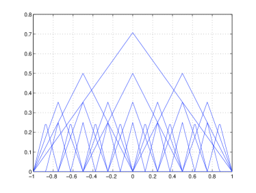
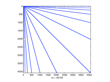
Figure 3: Left: four levels of hat functions on the interval $[-1,1]$. Right: nonzeros in the corresponding stiffness matrix with $11$ levels.

We apply a finite element method [5] and use classical shape functions

$$\phi(x):=\begin{cases}1-\lvert{x}\rvert&\text{if }-1\leq x\leq 1\\ 0&\text{otherwise.}\end{cases}$$ (30)

The different refinement levels are given by

$$\phi_{k,\ell}(x):=2^{-k/2}\,\phi\big{(}2^{k-1}\,(x+1)-\ell\big{)},\ k\in\mathbb{N},\;\ell=1,\dots,2^{k}-1.$$

Here, the scaling factor $2^{-k/2}$ is used to make the diagonal elements of the stiffness matrix equal to $1$. We then have

$$\phi_{k,\ell}(x)=2^{-k/2}\begin{cases}1-\lvert{2^{k-1}\,(x+1)-\ell}\rvert&\text{if }-1+\frac{\ell-1}{2^{k-1}}\leq x\leq-1+\frac{\ell+1}{2^{k-1}}\\ 0&\text{otherwise,}\end{cases}$$

see the left part of Figure 3 for an illustration. On the $N$th level, we then have

$$\sum_{k=1}^{N}(2^{k}-1)=2^{N+1}-(N+2)$$

generating functions and we obtain a stiffness matrix that has a sparsity as depicted on the right part of Figure 3.

For this problem we have numerically computed the mutual incoherence and the restricted isometry constant. The numerical results indicate that for $A^{N-n,N}$ as in (17) we have

$$\mathcal{M}(A^{N-n,N})=\sqrt{\tfrac{2}{3}},$$

independently of the size of the matrices, and that $\delta_{1}=0$, $\delta_{2}=0.8165$, and for all $k>1$, we have $\delta_{k}>1$.

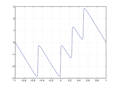
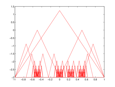
Figure 4: Left: exact solution and approximate solution of the example in Section 5.1 at level 8. Right: hat functions that are selected by the $\ell_{1}$-minimization problem.

On level $8$ we used the matrix $A^{N-n,N}$ of size $255\times 502$. The least squares solution of $A^{N}x=b$ has 495 nonzeros, while the minimum $\ell_{1}$-solution only had 57 nonzeros. The left part of Figure 4 depicts the exact solution and the approximate solution at level $8$. There is no obvious difference and the relative error in $\ell_{2}$-norm is $0.0627$. The right part of Figure 4 shows that our method refines properly at points with large gradients.

5.2 Application of Algorithm 1 to a 1D-Poisson Equation

To illustrate the behavior of Algorithm 1, we consider the Poisson equation

$$\begin{array}[]{l l}Lu=-u^{\prime\prime}=2\frac{(100\pi)^{3}x}{1+(100\pi x)^{2}}+2\frac{(100\pi)^{3}(x-0.5)}{1+(100\pi(x-0.5))^{2}},\quad x\in\Omega=(-1,1),\\ (u(-1),u(1))=(0,0).\end{array}$$ (31)

The exact solution of this problem is

$$u= \arctan(100\,\pi\cdot x)+\arctan(-100\,\pi)\cdot x$$

$$+\arctan(100\,\pi(x-\tfrac{1}{2}))+\arctan(-100\,\pi)(x-\tfrac{1}{2}).$$

We applied four refinement steps of Algorithm 1 starting from level 4. In turns out that starting from level 3, a straightforward refinement process does not work, since some of the singularities are lost; this is a point where our algorithm would need to backtrack, see Section 3.2.

For the starting level $4$, the size of matrix $A_{11}$ in (13) is $2^{r}-(r+1)=11$ for $r=4$. The size of $A_{21}$ is $(2^{r}-1)\times(2^{r}-(r+1))=15\times 11$. The size of $A_{22}$ is $15\times 15$.

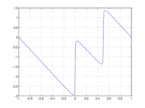
Figure 5: Exact and approximate solution for Example 5.2 using Algorithm 1.

Table 1: Results of Algorithm 1 for Example 5.2. The first column is the refinement step, column 2 gives the size of the matrix used for the $\ell_{1}$-minimization problem, column 3 gives the $\ell_{0}$-norm of the $\ell_{1}$-minimal solution, column 4 gives the size of the matrix used for the classical FEM, column 5 gives the FEM solution of the problem at different levels, and column 6 gives the ratio of $\ell_{0}$-norms of the $\ell_{1}$-solution and the FEM solution.

step	size of $\ell_{1}$-matrix	$\lVert{z}\rVert_{0}$	size of FEM matrix	$\lVert{x}\rVert_{0}$	$\lVert{z}\rVert_{0}/\lVert{x}\rVert_{0}$
1	15 $\times$ 26	13	15 $\times$ 15	15	0.867
2	29 $\times$ 42	23	31 $\times$ 31	31	0.742
3	59 $\times$ 72	41	63 $\times$ 63	63	0.651
4	113 $\times$ 126	67	127 $\times$ 127	127	0.528
5	191 $\times$ 204	103	255 $\times$ 255	255	0.404

At each step we determine the new support using $\ell_{1}$-minimization and then refine these nodes and all necessary higher level nodes according to Algorithm 1, see Figure 5. In Table 1 we present the results of four refinement steps of Algorithm 1.

5.3 Application of Algorithm 1 to a 2D-Poisson Equation

As a second example for Algorithm 1, we consider the Poisson equation

$$-\frac{\partial^{2}u}{\partial x^{2}}-\frac{\partial^{2}u}{\partial y^{2}}=f(x,y)\ \text{on}\ [0,1]\times[0,1]$$

with $u(x,y)=0$ on the boundary of $[0,1]\times[0,1]$ where $f(x,y)=-20x(x-1)-20y(y-1)$. The original solution is $u(x,y)=10xy(x-1)(y-1)$.

Figure 6: Triangulation on first and second level

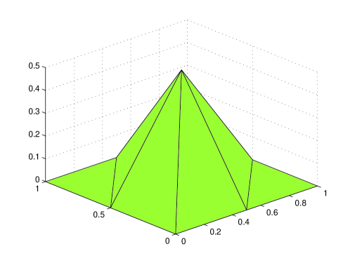
Figure 7: Basis function in the first level

We use piecewise linear generating functions of the form $u_{i}(x,y)=a_{i}x+b_{i}y+c_{i}$ on each triangle. Figure 6 depicts the refinement step from the first level (left) to the second level (right). The basis function on level 1 is plotted in Figure 7.

Based on the triangulation on level $j$ and the triangles $\{\Delta_{j,k_{i}}\}_{i=1}^{6}$, we obtain the generating functions:

$$\phi_{j,(a,b)}(x,y)=\frac{1}{2}\begin{cases}2^{j}(x-a)+1&(x,y)\in\Delta_{j,k_{1}}\\ 2^{j}(x-a)-2^{j}(y-b)+1&(x,y)\in\Delta_{j,k_{2}}\\ -2^{j}(y-b)+1&(x,y)\in\Delta_{j,k_{3}}\\ -2^{j}(x-a)+1&(x,y)\in\Delta_{j,k_{4}}\\ -2^{j}(x-a)+2^{j}(y-b)+1&(x,y)\in\Delta_{j,k_{5}}\\ 2^{j}(y-b)+1&(x,y)\in\Delta_{j,k_{6}}\\ \end{cases}$$

where $(a,b)$ is the center of the basis function. In general on level $n$ we have $(2^{n}-1)^{2}$ basis functions.

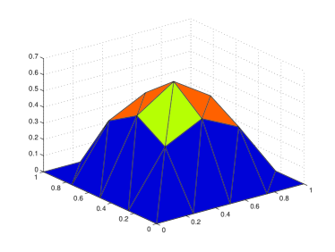
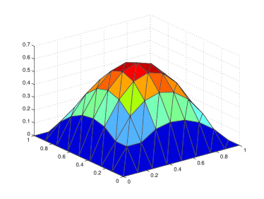
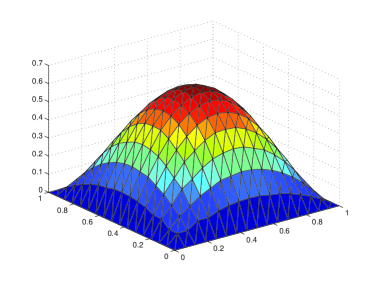
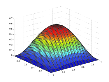
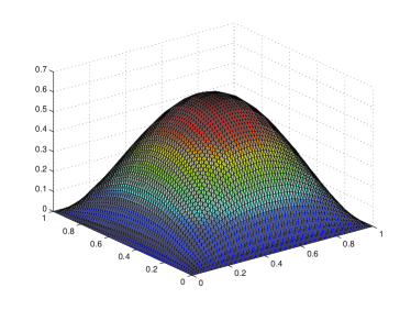
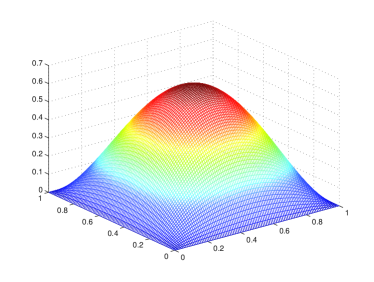
Figure 8: Approximate solutions obtained by Algorithm 1 on levels $2,3,4,5,6$ and exact solution (last) for Example 5.3.

Table 2: Results of Algorithm 1 for Example 5.3. The first column is the refinement step, column 2 gives the size of the matrix used for the $\ell_{1}$-minimization problem, column 3 gives the $\ell_{0}$-norm of the $\ell_{1}$-minimal solution, column 4 gives the size of the matrix used for the classical FEM, column 5 gives the FEM solution of the problem at different level, and column 6 gives the ratio of $\ell_{0}$-norms of the $\ell_{1}$-solution and the FEM solution.

step	size of $\ell_{1}$-matrix	$\lVert{z}\rVert_{0}$	size of FEM matrix	$\lVert{x}\rVert_{0}$	$\lVert{z}\rVert_{0}/\lVert{x}\rVert_{0}$
1	9 $\times$ 10	8	9 $\times$ 9	9	0.889
2	43 $\times$ 51	42	49 $\times$ 49	49	0.857
3	237 $\times$ 244	114	225 $\times$ 225	225	0.507
4	816 $\times$ 823	172	961 $\times$ 961	961	0.179
5	1352 $\times$ 1359	190	3969 $\times$ 3969	3969	0.048

We applied four refinement steps of Algorithm 1 starting as first step from level 2. At each step we determine the new support using $\ell_{1}$-minimization and then refine these nodes and all necessary higher level nodes according to Algorithm 1 (see Figure 8). In Table 2 we present the results of four refinement steps of Algorithm 1. For the starting level $2$, the size of matrix $A_{11}$ in (13) is $\sum_{i=1}^{r-1}(2^{i}-1)^{2}=1$ for $r=2$. The size of $A_{21}$ is $(2^{r}-1)^{2}\times\sum_{i=1}^{r-1}(2^{i}-1)^{2})=9\times 1$. The size of $A_{22}$ is $9\times 9$.

6 Efficiency Estimation

The algorithm as described in Section 3.2 relies on the solution of a linear program (LP) in each iteration. Thus, for it to be successful in practice the savings in the size of the matrices have to be large enough to compensate for the higher solution times of LPs compared to the standard finite element methods. Clearly, this depends on a number of factors that are hard to predict: the PDE, the data, the required accuracy, the concrete implementation, the usage of geometric refinement processes etc. This results in different sizes of the refinement tree and different matrices with varying degrees of sparsity. We will nevertheless try to get a rough idea of the efficiency. Since our method can be seen as a generic way of controlling the refinement process, we compare it against the classical finite element method without refinement. We use the examples of Section 5 as a guideline.

Note that we restrict our attention to the case of solving LPs, although there are different methods for compressed sensing that yield similar results as the LP-based methods; for instance, orthogonal matching pursuit might be applied, see Tropp [41], Donoho, Elad, and Temlyakov [25], Tropp and Gilbert [43] and Needell and Tropp [35]. It remains to be seen whether these methods are competitive for the application discussed in this paper, especially with respect to sparse matrices.

Let us first consider worst case computing times. In the example in Section 5.1, the number of basis functions at level $k$ is $2^{k}-1$, which is also the size of the matrix $A^{k}$ in the equation system (12), which has to be solved by a “classical” finite element method. If we use a dense solver this takes $O(2^{3k})$ time for each solution. In comparison, dense interior point algorithms for linear programming require about $O(n^{3.5}L)$ time for an LP of dimension $n$, where $L$ is the encoding size of the LP. If the LP is dense, the encoding length includes at least one bit for each entry of the matrix and thus is of size at least $nm$, where $m$ is the number of constraints. In our case, we have $n=2^{k+1}-(k+2)$ and $m=2^{k}-1$, if we would start our method at level $k$. Hence, a very optimistic estimate of the running time in the dense case would be $O(n^{3.5}mn)=O(2^{5.5k})$.

Table 3: Running times for solving the LPs of the example in Section 5.1; $m$ and $n$ denote the number of rows and columns of the constraint matrix, “time” refers to the running time in seconds, and $\lVert{z}\rVert_{0}$ gives the number of nonzeros in the solution.

level	$m$	$n$	time	$\lVert{z}\rVert_{0}$
7	127	247	0.01	7
8	255	502	0.03	8
9	511	1013	0.10	9
10	1023	2036	0.46	10
11	2047	4083	1.68	11
12	4095	8178	5.74	12
13	8191	16369	22.24	13
14	16383	32752	88.32	14

Let us investigate the selection process of the compressed sensing approach for this example, see Section 3.2. Assume that we are at iteration $k$ and we have the set $C^{k-1}$ of basis functions with $\ell_{k-1}=\#\,{C^{k-1}}$. The refined set of basis functions $\hat{C}^{k}$ has size at most $3\,\ell_{k-1}$, because each basis function is subdivided into three new basis functions (some of the new basis functions might coincide). Assuming that we select at least a fraction of $\alpha\in(0,1]$ among the basis functions of $\hat{C}^{k}$, the new iteration has at most $\ell_{k}=\ell_{k-1}+\alpha\,3\,\ell_{k-1}=(1+3\,\alpha)\ell_{k-1}$ basis functions; compare Algorithm 1. Therefore, at iteration $k$, we have at most $(1+3\alpha)^{k}=2^{k\log_{2}(1+3\alpha)}$ basis functions. For the compressed sensing approach to be successful with respect to the finite element (dense) worst case times above, we would need

$$\log_{2}(1+3\alpha)<3.5/5.5\approx 0.64$$

$$\Leftrightarrow\quad \alpha<\tfrac{1}{3}\,(2^{0.64}-1)\approx 0.19.$$

Hence, if we assume that the compressed sensing method yields a reduction rate $\alpha$ below approximately $0.19$, it should be effective, if we assume worst case running times. In the results of Table 1, we have $\alpha$ around $0.5$.

Figure 9: Solution times for solving the linear programs of Table 3 versus the number of columns of the matrix.

The above estimation is based on the dense worst case running times. Since the matrix is sparse, we can rather assume that the running times for solving the equation system are about linear with respect to the size [1, 4, 40]. To estimate the running time for linear programming, we have to resort to experiments based on the data of Section 5.1. We use the matrices as they would result from starting our algorithm at levels 7 to 14. The results are shown in Table 3 and Figure 9. We used the barrier solver of CPLEX with additional crossover to recover a basic solution. The running times are with respect to an Intel Core 2 Quad Core with 2.66 GHz. In Table 3, $\alpha$ seems to be of order $\alpha\approx k$. Moreover, the results suggest a growth of the running time that is lower than quadratic. This seems to be a positive sign, which at least does not rule out a possible practical effectiveness of our approach. It, however, would require a much more thorough computational study to reach definite conclusions.

Conclusion

As mentioned in the introduction, many issues of the approach presented in this paper have not yet been resolved and many variations are possible. For instance, it is obvious that a similar approach could be derived using other dictionaries, e.g., wavelets, instead of finite element functions. Furthermore, for practical instances, the solution of the $\ell_{1}$-minimization problem becomes an issue. One approach would be to apply different algorithms, for instance, Orthogonal Matching Pursuit, see [19, 37, 36]. Moreover, the special structure of the stiffness matrices can be exploited and techniques adapted to the iterative procedure could be developed.

References

- [1] P. R. Amestoy, A. Guermouche, J.-Y. L’Excellent, and S. Pralet, Hybrid scheduling for the parallel solution of linear systems, Parallel Computing 32, no. 2 (2006), pp. 136–156.
- [2] R. Baraniuk, Optimal tree approximation using wavelets, in SPIE Technical Conference on Wavelet Applications in Signal Processing, Denver, CO, July 1999.
- [3] R. Becker and R. Rannacher, An optimal control approach to a posteriori error estimation in finite element methods, in Acta Numerica, no. 10, Cambridge University Press, 2001, pp. 1–102.
- [4] S. Börm, L. Grasedyck, and W. Hackbusch, Hierarchical matrices, tech. report, Lecture Note 21 of the Max Planck Institute for Mathematics in the Sciences, 2003.
- [5] D. Braess, Finite Elements: Theory, Fast Solvers and Applications in Solid Mechanics, Cambridge, Cambridge University Press, 3rd ed., 2007.
- [6] E. J. Candés, Compressive sampling, in Proc. International Congress of Mathematics, Madrid, Spain, 2006, pp. 1433–1452.
- [7] E. J. Candès, The restricted isometry property and its implications for compressed sensing, CR Math. Acad. Sci. Paris, 346, no. 9–10 (2008), pp. 589–592.
- [8] E. J. Candès and J. Romberg, Quantitative robust uncertainty principles and optimally sparse decompositions, Found. Comput. Math. 6, no. 2 (2006), pp. 227–254.
- [9] E. J. Candès, J. Romberg, and T. Tao, Robust uncertainty principles: Exact signal reconstruction from highly incomplete frequency information, IEEE Trans. Inform. Theory 52, no. 2 (2006), pp. 489–509.
- [10] E. J. Candès, J. Romberg, and T. Tao, Stable signal recovery from incomplete and inaccurate measurements, Comm. Pure Appl. Math. 59, no. 8 (2006), pp. 1207–1223.
- [11] E. J. Candès and T. Tao, Decoding by linear programming, IEEE Trans. Inform. Theory 51, no. 12 (2005), pp. 4203–4215.
- [12] E. J. Candès and T. Tao, Near-optimal signal recovery from random projections: Universal encoding strategies, IEEE Trans. Inform. Theory 52, no. 12 (2006), pp. 5406–5425.
- [13] S. S. Chen, Basis Pursuit, PhD thesis, Department of Statistics, Department of Statistics, Stanford,CA, 1995.
- [14] S. S. Chen, D. L. Donoho, and M. A. Saunders, Atomic decomposition by basis pursuit, SIAM J. Sci. Comput. 20, no. 1 (1999), pp. 33–61.
- [15] O. Christensen, An introduction to frames and Riesz bases, Birkhäuser, Boston, 2003.
- [16] A. Cohen, W. Dahmen, I. Daubechies, and R. DeVore, Tree approximation and optimal encoding, Appl. Comput. Harmonic Analysis 11, no. 2 (2001), pp. 192–226.
- [17] A. Cohen, W. Dahmen, and R. DeVore, Adaptive wavelet methods for elliptic operator equations: convergence rates, Math. Comput. 70, no. 233 (2001), pp. 27–75.
- [18] A. Cohen, W. Dahmen, and R. DeVore, Compressed sensing and best k-term approximation, J. Amer. Math. Soc. 22 (2009), pp. 211–231.
- [19] G. Davis, S. Mallat, and Z. Zhang, Adaptive time-frequency decompositions with matching pursuits, Opt. Eng. 33, no. 7 (1994), pp. 2183–2191.
- [20] R. A. DeVore, Deterministic constructions of compressed sensing matrices, Journal of Complexity 23 (2007), pp. 918–925.
- [21] D. L. Donoho, Compressed sensing, IEEE Trans. Inform. Theory 52, no. 4 (2006), pp. 1289–1306.
- [22] D. L. Donoho, For most large underdetermined systems of equations, the minimal -norm near-solution approximates the sparsest near-solution, Comm. Pure Appl. Math. 59, no. 7 (2006), pp. 907–934.
- [23] D. L. Donoho, For most large underdetermined systems of linear equations the minimal -norm solution is also the sparsest solution, Comm. Pure Appl. Math. 59, no. 6 (2006), pp. 797–829.
- [24] D. L. Donoho and M. Elad, Optimally sparse representation in general (nonorthogonal) dictionaries via minimization, Proc. Natl. Acad. Sci. USA 100, no. 5 (2003), pp. 2197–2202.
- [25] D. L. Donoho, M. Elad, and V. Temlyakov, Stable recovery of sparse overcomplete representations in the presence of noise, IEEE Trans. Inform. Theory 52, no. 1 (2006), pp. 6–18.
- [26] D. L. Donoho and X. Huo, Uncertainty principles and ideal atomic decomposition, IEEE Trans. Inform. Theory 47, no. 7 (2001), pp. 2845–2862.
- [27] D. L. Donoho, Y. Tsaig, I. Drori, and J.-L. Starck, Sparse solution of underdetermined linear equations by stagewise orthogonal matching pursuit, Tech. Report 2006-02, Standford, Department of Statistics, 2006.
- [28] M. R. Garey and D. S. Johnson, Computers and Intractability. A Guide to the Theory of NP-Completeness, W. H. Freeman and Company, New York, 1979.
- [29] R. A. Horn and C. R. Johnson, Matrix analysis, Cambridge University Press, New York, NY, USA, 1986.
- [30] S. Jokar and M. Pfetsch, Exact and approximate sparse solutions of underdetermined linear equations, SIAM J. Sci. Comput. 31, no. 1 (2008), pp. 23–44.
- [31] N. Karmarkar, A new polynomial-time algorithm for linear programming, Combinatorica 4, no. 4 (1984), pp. 373–395.
- [32] L. G. Khachiyan, A polynomial algorithm in linear programming, Soviet Math. Dokl. 20 (1979), pp. 191–194.
- [33] S. Kunis and H. Rauhut, Random sampling of sparse trigonometric polynomials II – orthogonal matching pursuit versus basis pursuit, Foundations of Computational Mathematics 8, no. 6 (2008), pp. 737–763.
- [34] B. K. Natarajan, Sparse approximate solutions to linear systems, SIAM J. Comput. 24, no. 2 (1995), pp. 227–234.
- [35] D. Needell and J. A. Tropp, CoSaMP: Iterative signal recovery from incomplete and inaccurate samples. Accepted to Appl. Comp. Harmonic Anal., June 2008.
- [36] D. Needell and R. Vershynin, Uniform uncertainty principle and signal recovery via regularized orthogonal matching pursuit. Foundations of Computational Mathematics, DOI: 10.1007/s10208-008-9031-3, 2008.
- [37] Y. C. Pati, R. Rezaiifar, and P. S. Krishnaprasad, Orthogonal matching pursuit: Recursive function approximation with applications to wavelet decompositions, in Proc. 27th Asilomar Conference on Signals, Systems and Computers, A. Singh, ed., 1993.
- [38] H. Rauhut, Random sampling of sparse trigonometric polynomials, Appl. Comput. Harmonic Analysis 22, no. 1 (2007), pp. 16–42.
- [39] H. Rauhut, Stability results for random sampling of sparse trigonometric polynomials, IEEE Trans. Inform. Theory 54, no. 12 (2008), pp. 5661–5670.
- [40] O. Schenk, A. Wächter, and M. Weiser, Inertia-revealing preconditioning for large-scale nonconvex constrained optimization, SIAM J. Sci. Comput. 31, no. 2 (2008), pp. 939–960.
- [41] J. A. Tropp, Greed is good: algorithmic results for sparse approximation, IEEE Trans. Inform. Theory 50, no. 10 (2004), pp. 2231–2242.
- [42] J. A. Tropp, Just relax: convex programming methods for identifying sparse signals in noise, IEEE Trans. Inform. Theory 52, no. 3 (2006), pp. 1030–1051.
- [43] J. A. Tropp and A. C. Gilbert, Signal recovery from random measurements via orthogonal matching pursuit, IEEE Trans. Inform. Theory 53, no. 12 (2007), pp. 4655–4666.