Non-thermal Dark Matter and the Moduli Problem
in String Frameworks
Abstract:
We address the cosmological moduli/gravitino problems and the issue of too little thermal but excessive non-thermal dark matter from the decays of moduli. The main examples we study are the -MSSM models arising from theory compactifications, which allow for a precise calculation of moduli decay rates and widths. We find that the late decaying moduli satisfy both BBN constraints and avoid the gravitino problem. The non-thermal production of Wino LSPs, which is a prediction of -MSSM models, gives a relic density of about the right order of magnitude.
MCTP-08-10
1 Introduction
The existence of Dark Matter seems to require physics beyond the Standard Model. If this physics arises from a string/ theory vacuum, one is faced with various problems associated with the moduli fields, which are gauge-singlet scalar fields that arise when compactifying string/ theory to four dimensions. In particular, moduli fields can give rise to disastrous cosmological effects.
For example, the moduli have to be stabilized, or made massive, in accord with cosmological observations. Even if these moduli are made massive, there could be a large amount of energy stored in them leading to the formation of scalar condensates. In most cases, this condensate will scale like ordinary matter and will quickly come to dominate the energy density. The moduli are unstable to decays to photons, and when this occurs, the resulting entropy can often spoil the successes of big-bang nucleosynthesis (BBN). This is the cosmological moduli problem [1, 2, 3, 4, 5]. In supersymmetric extensions of the standard model, the overproduction of gravitinos can cause similar problems and have been a source of much investigation [6, 7, 8, 19, 16, 17, 18, 9, 10, 11, 12, 14, 13, 15].
In addition, the “standard” picture in which Dark Matter (DM) particles are produced during a phase of thermal equilibrium can be significantly altered in the presence of moduli. The moduli, which scale like non-relativistic matter, typically dominate the energy density of the Universe making it matter dominated. Therefore, the dominant mechanism for production of DM particles is non-thermal production via the direct decay of moduli777For other phenomenologically based approaches to non-thermal dark matter and the related issue of baryon asymmetry in the presence of scalar decay see [20, 22, 21].. However, this can lead to further problems since it is easy to produce too much dark matter compared with what we observe today.
In recent years there has been considerable progress in our understanding of moduli dynamics and their potential in different frameworks which arise in various limits of string/ theory. The most popular examples include the KKLT and Large Volume frameworks in Type IIB string theory [23, 24, 25], where all moduli are stabilized by a combination of fluxes and quantum corrections. These frameworks are also attractive in the sense that they provide a mechanism for supersymmetry breaking at low scales (), thus accommodating the hierarchy between the Electroweak and Planck scales (see [26, 27, 28] for reviews). Since one can concretely study the couplings between moduli and matter fields, we have an opportunity to address many issues in particle physics and cosmology from an underlying microscopic viewpoint. The cosmological moduli/gravitino problems and adequate generation of dark matter within the Type IIB frameworks has met with some mixed success in a recent paper [29].
In this paper we will study a different framework, in which we will also address the Dark Matter and moduli/gravitino problems. This is the low energy limit of theory vacua in which the extra dimensions form a manifold of holonomy. Although the study of such vacua has proven to be technically challenging, much progress has been made towards understanding the effective four dimensional physics emerging from them [31, 32, 33, 34]. This includes many phenomenological implications of these vacua, in particular relating to issues such as constructing a realistic visible sector with chiral matter and non-abelian gauge bosons, supersymmetry breaking, moduli stabilization in a dS vacuum as well as explaining the Hierarchy between the Electroweak and Planck scales, as exemplified in a number of works [30, 35, 36, 37, 38, 39].
We will show that the moduli, gravitino and dark matter problems are all naturally solved within this framework. Because of the presence of moduli, the Universe is matter-dominated from the end of inflation to the beginning of BBN. The LSPs are mostly produced non-thermally via moduli decays. The final result for the relic density only depends on the masses and couplings of the lightest of the moduli (which decay last) and the mass of the LSP. This is related to the fact that the LSP is a Wino in the -MSSM and that there is a fairly model independent critical LSP density at freeze out. For natural/reasonable choices of microscopic parameters defining the framework, one finds that it is possible to obtain a relic density of the right order of magnitude (up to factors of ). With a more sophisticated understanding of the microscopic theory, one might obtain a more precise result. The qualitative features which are crucial in solving the above problems may also be present in other realistic string/ theory frameworks.
Moduli which decay into Wino LSPs have been considered previously in the context of Anomaly Mediated Supersymmetry Breaking Models (AMSB) by Moroi and Randall [40]. The moduli and gaugino masses they consider are qualitatively similar to those of the -MSSM. There are some important differences however. In particular, the MSSM scalar masses in the [40] are much lower than the -MSSM, leading to much fewer LSPs produced per modulus decay compared to the models. Furthermore, unlike in AMSB, in the case one is able to calculate all the moduli masses and couplings explicitly which leads to a more detailed understanding. In essence, though, many of the important ideas in our work are already present in [40]. The -MSSM models can be thought of as a concrete microscopic realization of the relevant qualitative features of the AMSB models.
Interestingly, our actual result for the relic density (equation 59) is a few times larger than the WMAP value if we use central values for the microscopic constants, which should probably be regarded as a success. It is also worth remarking that, contrary to common views, it is not at all possible to get any value one wants – we can barely accommodate the actual observed value in the framework.
The paper is organized as follows. In Section 2 we briefly summarize early universe cosmology in the presence of moduli, and address many of the issues associated with their stabilization and decay. In Section 3 we give a non-technical overview of the main results. This is largely because much of this paper involves technical calculations. In section 4 we present a brief review of the -MSSM, a model which arises after considering moduli stabilization within the framework of theory compactifications. A basic discussion of decay rates and branching ratios for the moduli and gravitinos in this model follows, with a detailed calculation left for Appendix B. Then in section 5, we consider again the cosmology of moduli presented in section 2) for the case of the -MSSM. In section 6, after a review of dark matter production in both the thermal and non-thermal cases, we consider the dark matter abundance arising from the non-thermal decay of the -MSSM moduli. This section is a more technical overview of the salient features of dark matter production, leaving an even more detailed treatment for Appendix A. In this section we present our main result, which is that the -MSSM naturally predicts a relic density of Wino-like neutralinos of about the right magnitude in agreement with observation. This is followed by a detailed discussion of the results obtained and how it depends on the qualitative (and quantitative) features of the underlying physics. We then conclude with considerations for the future.
2 Early Universe Cosmology in the Presence of Moduli
Before considering the particular case of moduli in the -MSSM, we first briefly review the early universe evolution of moduli and the associated cosmological issues that can result. This section will also serve to set our conventions.
Currently, the only convincing model leading to a smooth, large, and nearly isotropic Universe as well as providing a mechanism for generating density perturbations for structure formation is cosmological inflation. At present we have very little understanding of how the “inflationary era” might arise within the theory framework. In what follows,therefore, we will assume that adequate inflation and (p)reheating have taken place and focus on the post-reheating epoch. We will also conservatively take the inflationary reheat temperature to be near the unification scale GeV, so that possibilities for high-scale baryogenesis exist. We will comment more on this issue at the end.
During inflation, the moduli fields are generically displaced from their minima by an amount of [41]. This can be seen by looking at the following generic potential experienced by the moduli:
| (1) |
where is the true vacuum-expectation-value (vev) of the field, i.e. in the present Universe. Only the first term in (1) comes from zero-temperature supersymmetry breaking, the other two highlight the importance of high-scale corrections and the mass-squared parameter () which results from the finite energy density associated with cosmological inflation [41]. As argued earlier, the potential (1) is dominated by the last two terms during inflation since . Thus, a minimum of the potential will occur near:
| (2) |
Here, for simplicity, we have implicitly assumed that the induced mass-squared parameter for during inflation is negative and of . This is possible for a non-minimal coupling between the inflationary fields and the moduli, a generic possibility within string theory. A large displacement of moduli fields is also possible when the induced mass-squared parameter during inflation is positive, but much smaller than . In this case, large dS fluctuations can drive the moduli fields to large values during inflation. Therefore, independent of details, the assumption we make is that gauge singlet scalar fields like moduli (and meson fields in the -MSSM) will be displaced from their present minimum by large values.
After the end of inflation and subsequent cosmological evolution, when , the soft mass term in the potential will dominate and we have:
| (3) |
is also typically of order . In Section 4, we will present the soft masses and decay rates for the moduli arising from soft SUSY breaking in the -MSSM low-energy effective theory relevant in the present Universe. Thus, we see that by considering moduli in the early universe with high-scale inflation, it is a rather generic consequence to expect moduli to be displaced from their low-energy (present) minimum by an amount:
| (4) |
2.1 Addressing the “Overshoot Problem”
The evolution of moduli after the end of inflation is governed by the following equation:
| (5) |
where the modulus decay rate is given by:
| (6) |
which reflects the fact that the modulus is gravitationally coupled () and is a model dependent constant that is typically order unity. After the end of inflation, the Universe is dominated by coherent oscillations of the inflaton field and . After the decay of the inflaton and subsequent reheating at temperature , the Universe is radiation dominated and . In both these phases, the evolution of the moduli can be written as:
| (7) |
where we have neglected as it is planck suppressed. The minimum of the potential now is time-dependent due to the time dependence of the Hubble parameter. The evolution of the moduli in the presence of matter and/or radiation as in the case above, has been studied in [42, 43, 44, 45, 46, 49, 50, 47, 48, 51]. In this case, as the modulus begins to roll down the potential, it was shown in [42, 45, 46, 47]) that the presence of matter/radiation has a slowing effect on the evolution of the field. This can naturally allow for the relaxation of moduli into coherent oscillations about the time-dependent minimum888We thank Joe Conlon and Nemanja Kaloper for discussions on this approach.. This ‘environmental relaxation’ can then slowly guide the modulus to the time-dependent minimum.
Another possibility arises if the minimum of the potential is located at a point of enhanced symmetry where additional light degrees of freedom become important. This naturally arises in SUGRA theories that are derived from string theories, where an underlying knowledge of the UV physics is known [52, 49, 50, 53]. If the modulus initially has a large kinetic energy, as it evolves close to the point of enhanced symmetry, new light degrees of freedom will be produced and then backreact to pull the modulus back to the special point of enhanced symmetry. This simple example of ‘moduli trapping’ is present in a large number of examples in string theory with points of enhanced symmetry [49, 50, 48, 51].
The above effects lead to a natural solution of the so-called ‘overshoot problem’ [54] (see also [55]), as argued below. As the universe expands and cools, the Hubble parameter () decreases until it eventually drops below the mass of the modulus (). Thus, from (1), we see that the first term in the potential now becomes of the same order as the other two terms and can no longer be neglected. At this time the modulus field becomes under-damped and begins to oscillate freely about the true minimum with amplitude . As an example, for , is leading to a potential value which is much smaller than the overall height of the potential barrier at this time (, as in any soft susy breaking potential). Thus, there is no overshoot problem.
The modulus will now quickly settle into coherent oscillations at a time roughly given by . After coherence is achieved, the scalar condensate will then evolve as pressure-less matter999If there are additional terms that contribute to the potential (besides the soft mass), then a coherently oscillating scalar does not necessarily scale as pressure-less matter., i.e. . Because the condensate scales as pressure-less matter , its contribution relative to the background radiation will grow with the cosmological expansion as . Thus, if enough energy is stored initially in the scalar condensate it will quickly grow to dominate the total energy density.
3 Overview of Results
This section reviews the main results of the paper without technical details.
As explained above, the moduli start oscillating when the Hubble parameter drops below their respective masses. Then they eventually dominate the energy density of the Universe before decaying. Within the context of -MSSM models, the relevant field content is that of the MSSM and real scalars. of these are the moduli, , of the -manifold and the remaining one is a scalar field, , called the meson field, which arises in the hidden sector dominating the supersymmetry breaking. A reasonable choice for would be - .
The masses are roughly as follows. The lightest particles beyond the Standard Model particles are the gauginos. In terms of the gravitino mass, , their masses are of order , suppressed by a small number . is determined by a combination of tree level and one-loop contributions which turn out to be comparable. The tree-level contribution is suppressed essentially because dominates the supersymmetry breaking, and to leading order, the gauge couplings are independent of . The precise spectrum of gaugino masses is qualitatively similar, but numerically different, to AMSB models. The LSP is a Wino in the -MSSM, similar to AMSB models. The current experimental limits on gauginos require that the gravitino mass is at least 10 TeV or so. In the framework, gravitinos naturally come out to be of TeV [38]. 50 TeV is a typical mass that we consider in this paper. The MSSM sfermions and higgsinos have masses of order , except the right handed stop which is a factor of few lighter due to RG running. Of the moduli, one, is much heavier than the rest, . The heavy modulus mass is about 600 , while the light moduli are essentially degenerate with masses 2. Finally the meson mass is also about 2. The decays of the moduli and meson into gravitinos will therefore be dominated by the heavy modulus .
The decays can be parameterized by the decay width as,
| (8) |
reflecting the fact that the decays are gravitationally suppressed. is a constant which we calculate to be order one for the moduli but order 700 for . So, the light moduli have decay widths of order eV, corresponding to a lifetime of order s. The heavier scalars have shorter lifetimes, s for and for , see tables 1 and 2. So, as the Universe cools further and reaches a value of order , the heavy modulus decays. When this happens, the Universe is reheated to a temperature, roughly of order GeV. The entropy is increased in this phase, by a factor of about . This greatly dilutes the thermal abundance of gravitinos and MSSM particles produced during reheating (by the inflaton). The abundance of the light moduli and meson are also diluted. Then, when reaches order the meson decays. This reheats the Universe to a temperature MeV and increases the entropy by a factor of order 100. Finally, as the Universe cools again and reaches a temperature of about eV the light moduli decay. They reheat the Universe to a temperature of about 30 MeV and a dilution factor of about 100 again. After this, all the moduli have decayed and the energy density is dominated by the decay of the light moduli. Since the final reheat temperature is well above that of nucleosynthesis, BBN can occur in the standard way.
Furthermore, since the entropy increases by a total factor of about , the gravtino density produced by moduli and meson decays is sufficiently diluted to an extent that it avoids existing bounds from BBN from gravitino decays.
Since the energy density is dominated by the decaying light moduli, the relic density of Wino LSP’s is dominated by this final stage of decay. The initial density of LSP’s at the time of production is such that the expansion rate is not large enough to prevent self-interactions of LSP’s. This is because
| (9) |
where the right side is to be evaluated at the final reheating temperature and is the typical Wino annihilation cross-section . Therefore, the Wino’s will annihilate until they reach the density given on the R.H.S., which is roughly eV3 - an energy density of eV4. Here we have assumed, as is reasonable, that since there is a lot of radiation produced at the time of decay, the LSPs quickly become non-relativistic by scattering with this ‘background’. Since the entropy at the time of the last reheating eV3, the ratio of the energy density to entropy, is around 1 eV. This should be compared to the observed value of this ratio today, which is 3.6 eV, where the Hubble parameter today is about 0.71.
Therefore, we see that the Wino LSP relic density is very reasonable in these models. The rest of this paper is devoted to a much more precise, detailed version of this calculation.
3.1 Scalar Decay and Reheating Temperatures
Here we collect some more precise formulae for the decay and reheat temperatures as a function of the moduli/meson masses.
The temperature at the time of decay can be found using
| (11) | |||||
where is the comoving number density and
| (12) |
is the entropy density with the number of relativistic degrees for freedom101010We will take , which is true if all particles track the photon temperature. This is a good approximation for most of the history of the universe (prior to decoupling) [56].. Parameterizing the decay rate as above, i.e. we find
| (13) |
For later use we also note that if more than one modulus dominates at the time of decay then the temperature at the time of decay becomes
| (14) |
where the sum is over all moduli (including the one that decays). When the modulus decays, the relativistic decay products will reheat the universe to a temperature,
| (16) | |||||
or
| (17) |
Instead, if more than one modulus contributes to the energy density before decay the reheat temperature becomes
| (18) |
where the sum is over all moduli (including the one that decays) and we note that this could lead to a subdominant radiation density compared to that of the remaining moduli. The entropy production is characterized by (assuming that )
| (19) |
where and are the decay and reheat temperatures, respectively. Making use of (17), (19), and (13) we find
| (20) | |||||
For the case that more than one modulus dominates the energy density before decays, we have instead
| (21) |
where the sum runs over all moduli that contribute to the energy density (including the decaying modulus ).
3.1.1 Moduli decay and BBN
From (21), we see that the decay of moduli can produce a substantial amount of entropy. Therefore, if any moduli present do not decay before the onset of BBN the resulting entropy production when decay occurs could result in devastating phenomenological consequences. However, another possibility is provided if the late-time decay of the moduli reheat the universe to temperatures greater than a few MeV. Such reheating will then allow BBN to proceed as usual. Requiring that the modulus decay exceeds this temperature one finds from (17) that TeV.
4 Summary of Results for the -MSSM
In this section, we give a brief summary of the results obtained in [37, 38, 39] for the -MSSM. Readers interested in more details should consult the references above. theory compactifications on singular manifolds are interesting in the sense that they give rise to supersymmetry in four dimensions with non-Abelian gauge groups and chiral fermions. The non-Abelian gauge fields are localized along three-dimensional submanifolds of the seven extra dimensions whereas chiral fermions are supported at points at which there is a conical singularity. In order to study phenomenology concretely one has to address the issues of moduli stabilization, supersymmetry breaking and generation of the Hierarchy between the Electroweak and Planck scales. These issues can be fairly successfully addressed within the above framework.
In [37, 38, 39], it was shown that all moduli can be stabilized generically in a large class of theory compactifications by non-perturbative effects. This happens in the zero-flux sector, our primary interest, when these compactifications support (at least two) non-abelian asymptotically free gauge groups. Strong gauge dynamics in these non-abelian (hidden sector) gauge groups gives rise to the non-perturbative effects which generate a moduli potential. When at least one of the hidden sectors also contains charged matter, under certain assumptions defining the above framework, supersymmetry is spontaneously broken in a metastable de Sitter vacuum which is tuned to the observed value. In the minimal framework, the hidden sector, including its moduli and hidden sector matter, is described by supergravity with the following Kähler potential , superpotential and gauge kinetic function at the compactification scale ():
| (22) |
Here is the volume of the manifold in units of the eleven-dimensional Planck length , and is a homogenous function of the of degree . A simple and reasonable ansatz therefore is with positive rational numbers subject to the constraint . is the effective meson field (for one pair of massless quarks) and and are proportional to one loop beta function coefficients of the two gauge groups which are completely determined by the gauge group and matter representations. The normalization constants and are calculable, given a particular -manifold. are the (tree-level) gauge kinetic functions of the two hidden sectors which have been taken to be equal for simplicity, (which is the case when the corresponding two 3-cycles are in the same homology class). are the geometric moduli of the manifold while are axionic111111These essentially decouple from the moduli stabilization analysis. Hence they will not be considered further. scalars. The integers are determined from the topology of the three-dimensional submanifold which supports the hidden sector gauge groups.
If volume of the submanifold supporting the hidden sector gauge theories () is large, the potential can be minimized analytically order-by-order in a expansion. Physically, this expansion can be understood as an expansion in terms of the small gauge coupling of the hidden sector – , which is self-consistent since the hidden sectors are assumed to be asymptotically free. The solution corresponding to a metastable minimum with spontaneously broken supersymmetry is given by
| (23) | |||||
| (24) |
where . The natural values of and are expected to lie between and . It is easy to see that a large corresponds to small for the hidden sector
| (25) |
implying that the expansion is effectively in . The dependence of the potential at the minimum is essentially
| (26) |
Therefore, the vacuum energy vanishes if the discriminant of the above expression vanishes, i.e. if
| (27) |
The above condition is satisfied when the contribution from the -term of the meson field () to the scalar potential cancels that from the term. In this vacuum, the -term of the moduli are much smaller than . Since phenomenologically interesting compactifications only arise for which corresponds to from (27), we will restrict our analysis to this particular choice.
4.1 Moduli Masses
Since in this paper we are interested in the evolution of the moduli (and meson) fields, it is important to study their masses in the vacuum described above. The set of gauge-singlet scalar fields includes geometric moduli associated with manifold and a hidden sector meson field . Since these moduli and meson will mix in general, the physical moduli correspond to mass eigenstates. The mass matrix can be written as:
| (28) | |||||
| (29) | |||||
| (30) |
where to are obtained in [38]:
| (31) | |||||
| (32) | |||||
| (33) | |||||
| (34) |
where . The special structure of the mass matrix allows us to find the eigenstates analytically. There is one heavy eigenstate with mass , degenerate light eigenstates with mass and an eigenstate with mass . These mass eigenstates of the moduli fields are given by:
| (35) |
where are the canonically normalized moduli fields. The normalized moduli fields can be related to the eigenstates by , in which can be constructed using the eigenstates listed above. It is easy to show that for the eigenvector . In addition, there is another eigenstate corresponding to the meson field. Actually, the heavy eigenstate and mix with each other. This mixing hardly changes the components of the eigenstate and since . However, the mass of the eigenstate is affected by the mixing. The masses and only have a mild dependence on (for ), and do not depend on the number of moduli at all. The mass of the light moduli does not even depend on . Taking the expression for , one immediately finds that . This result is very important since light moduli are then not allowed to decay into gravitinos, essentially eliminating the moduli induced gravitino problem. Choosing a reasonable value of to be of , one finds that is roughly around while is roughly around . Changing values of by hardly changes the moduli masses and . Therefore, the above typical values will be used henceforth in our analysis. To summarize, the meson and moduli masses in the -MSSM can be robustly determined in terms of .
4.2 Couplings and Decay Widths
Understanding the evolution of the moduli also requires a knowledge of the couplings of the moduli (meson) fields to the visible sector gauge and matter fields. Since all the moduli are stabilized explicitly in terms of the microscopic constants of the framework, all couplings of the moduli and meson fields to the MSSM matter and gauge fields can in principle be explicitly computed. Here we focus on the moduli couplings to MSSM matter and gauge fields. A different visible sector, as might arise from an explicit construction, will give rise to different couplings of the moduli fields in general, although with roughly the same moduli masses.
Here we will give a brief account of the important couplings of the moduli meson to visible gauge and matter fields and set the notation. Details are provided in Appendix B. The most important couplings of the moduli and meson fields involve two-body decays of the moduli and meson to gauge bosons, gauginos, squarks and slepton, quarks and leptons, higgses and higgsinos. The three-body decays are significantly more suppressed and will not be considered.
Let us start with the decay to gauge bosons and gauginos. The relevant part of the Lagrangian is given by:
| (36) | |||||
Here, , , and are the normalized moduli, meson, gauge field strength and gaugino fields respectively. The expression for the couplings will be provided in Appendix B. It is important to note that the meson field does not couple to gauge bosons since the gauge kinetic function does not depend on . The normalized moduli eigenstates have already been discussed. The others can be written as:
| (37) |
where is the gauge kinetic function for the visible SM gauge group. In the rest of the paper, we will neglect the hats for these normalized fields and in the couplings for convenience.
The coupling of the moduli and meson fields to the MSSM non-higgs scalars (ie sfermions) turn out to be important, as will be seen later. Since the Standard model fermion masses (including that of the top) are much smaller than that of the moduli, the decay of the moduli and meson to these fermions will not be considered. The coupling to the MSSM sfermions can be written as:
| (38) | |||||
where are the canonically normalized scalar components of the visible chiral fields , i.e. . The couplings to the higgs and higgsinos are different due to the presence of the higgs bilinear in the Kähler potential[39], which gives rise to contributions to the and parameters. In addition to the couplings similar as those in Eq.(107), there are additional couplings for scalar higgses, which can be schematically written as:
| (39) | |||||
As explained in [39], all higgs scalars except the SM-like higgs and all higgsinos are heavier than the gravitino, implying that the moduli and meson fields can only decay in this sector to the light SM-like higgs (). The coupling to the SM-like higgs can be determined from the above coupling as explained in appendix B.
Finally, the moduli and meson fields can also decay directly to the gravitino. In fact, it turns out that the (non-thermal) production of gravitinos from direct decays dominates the thermal production of gravitinos in the early plasma. Therefore, it is important to consider the moduli and meson couplings to the gravitinos. Since the meson and light moduli are lighter than twice the gravitino mass (as seen from the previous subsection), only the heavy modulus can decay to the gravitino.
The explicit form of these couplings in terms of the microscopic constants is provided in appendix B. An important point to note is that these couplings are computed from the theory at a high scale, presumably the unification scale. However, since the temperature at which the moduli decay is much smaller than the unification scale, one has to RG evolve these couplings to scales at which these moduli decay (around their masses). The RG evolution has also been discussed in appendix B for the important couplings. Once the effective couplings of these moduli and meson are determined, one can compute the decay widths, as shown below.
For the -MSSM model, we have found that light moduli and meson dominantly decay to light higgses and squarks, while the heavy modulus dominantly decay to light higgses only. In appendix B, we have explicitly calculated the decay widths of the moduli and meson. The widths of moduli can be schematically written as:
where and is the number of gauge bosons or gauginos. Note that is significant only for (see appendix B). For the meson, the width can be written as:
| (41) | |||||
4.3 Nature of the LSP
Before moving on to discuss the evolution of moduli in the -MSSM, it is important to comment on the nature of LSP in this framework. As explained in detail in [39], the -MSSM framework gives rise to Wino LSPs for choices of microscopic constants consistent with precision gauge unification. Therefore, in our analysis we focus on the Wino LSP case. As we will see, a Wino LSP turns out to be crucial in obtaining our final result.
5 Evolution of Moduli in the -MSSM
In this section, we apply the general discussion in Section 2 to the model of the -MSSM reviewed in the previous section. For clarity we will summarize our main results focusing on the more salient aspects of the physics, leaving the more technical details of the calculations to Appendix A. We will illustrate our computations with benchmark values, in order to get concrete numerical results, and comment on the choice of the benchmark values in section 7.
As discussed in Section 2, we assume that cosmological inflation and (p)reheating have provided adequate initial conditions for the post-inflationary universe.
5.1 Moduli Oscillations
As reviewed in the last section, we have a heavy modulus , light moduli , and the scalar meson . These will begin to oscillate in the radiation dominated universe once the temperature cools and the expansion rate becomes comparable to their masses.
For a benchmark gravitino mass value121212We give detailed numerical values for TeV. It will be clear that values a factor of two or so smaller or larger than this will not change any conclusions in this and related analyses. of TeV, the heavy modulus will begin oscillations first, at around seconds, corresponding to a temperature of roughly GeV. Following the heavy modulus, the other moduli will begin coherent oscillations around corresponding to a temperature of roughly GeV. These results are summarized in Table 1 below.
| Modulus | Mass ( TeV) | Oscillation Time (seconds) |
|---|---|---|
Since coherently oscillating moduli () scale relative to radiation as , the moduli will quickly come to dominate the energy density of the universe, which is then matter dominated. Following the beginning of coherent oscillations of the heavy modulus, until the decay of all the moduli the universe will remain matter dominated. We will see that this, along with the entropy produced during moduli decays, results in negligible primordial thermal abundances of (s)particles compared with the non-thermal abundances coming from direct decays of the moduli. This will be crucial in addressing the gravitino problem and establishing a Wino-like LSP as a viable dark matter candidate through its non-thermal production.
5.2 Moduli Decays and Gravitino Production
As the universe continues to cool the expansion rate will eventually decrease enough so that the moduli are able to decay. This occurs when , at which time the moduli will decay reheating the universe and producing substantial entropy. We will parameterize the decay rates of the -MSSM moduli as:
| (42) |
where is the decay width for particle . The decay times will be computed for a set of benchmark values of for the various moduli (meson) which can be obtained by choosing particular (reasonable) sets of values of the microscopic constants (see appendix B for details).
| Modulus | Decay constant | Decay Time (seconds) |
|---|---|---|
5.2.1 Heavy Modulus Decay and Initial Thermal Abundances
Given the -MSSM values in Table 2 above, the heavy modulus will be the first to decay at around . This decay will produce a large amount of entropy (even though the energy density of the heavy modulus is less than that of the meson and moduli), reheating the universe to a temperature GeV. The entropy production will not only dilute the thermal abundances of all (s)particles, but also all the other moduli. One particularly important non-relativistic decay product of the heavy modulus is the gravitino. Gravitinos will be non-thermally produced by the modulus decay with a branching ratio , which yields a comoving abundance . This can be compared to the thermal abundance of gravitinos, which before modulus decay is . This is further diluted by entropy production resulting from the decay, i.e. . We see that the thermal contribution to the gravitino abundance is negligible compared to that from non-thermal production. A similar result follows for all other (s)particles that are thermally populated following inflation. Therefore, the primary source of (s)particles, and in particular gravitinos and Lightest SUSY Particles (LSPs), will result from non-thermal production resulting from decays of the moduli.
5.2.2 Meson/Light Moduli Decays and the Gravitino Problem
The decay of the heavy modulus is followed by the decay of the meson, at around (for benchmark values). The meson will decay before the light moduli because of a larger decay width compared to that for the light moduli (see appendix B for details). Similar to the heavy modulus, the meson contribution to the energy density is small compared to that of the light moduli. Nevertheless, it produces some entropy () and reheats the universe to a temperature of around MeV. The entropy production will again dilute the abundance of light moduli, and any (s)particles present, including the gravitinos from the heavy modulus decay.
The decay of the meson to gravitinos is particularly important, as this can result in the well-known gravitino problem. If the scalar decay yields a large number of gravitinos, these gravitinos can later decay producing a substantial amount of entropy that could spoil the successes of BBN.
The entropy produced from the decay of the meson and the other light moduli further dilutes the gravitino abundance from the heavy modulus. The primary contribution to the gravitino relic abundance comes from the decay of the heavy modulus since the other fields have masses of order 2 . After the decay of the meson, the energy density of the light moduli is the dominant contribution to the total energy density of the Universe.
Given that the light moduli are approximately degenerate in mass, their decays will occur at nearly the same time, after the decay of the meson. The resulting reheat temperature is found to be approximately MeV, which is an acceptable temperature for consistency with the bound of MeV set by BBN [57, 58, 59, 60].
We note that the moduli decay rates have a strong dependence on the gravitino mass (as it sets the moduli mass scale). So, the decay of the light moduli being able to avoid BBN constraints is a result of the fact that the gravitino mass is relatively large ( TeV). However, as explained in detail in [39], the gauginos are significantly suppressed relative to the gravitinos allowing us to still obtain a light ( TeV) spectrum which can be seen at the LHC. The decay of each modulus will contribute to the total entropy production, and one finds that the total entropy production for the set of benchmark values of the microscopic constants is given by . We also note that the light moduli lifetime depends inversely on the decay constant , so if instead of taking relatively large values we take relatively small values , we find a reheat temperature of MeV which is still compatible with BBN131313See appendix A for a discussion of the range of the coefficients .. The decay of light moduli to gravitinos is kinematically suppressed for the same reason as for the meson. The final gravitino abundance is then just the contribution from the heavy modulus decay diluted by the decay of the meson and light moduli and is . The above gravitino abundance is well within the upper bound on the gravitino abundance set by BBN constraints, as it will not lead to any significant entropy production at the time the gravitinos decay. Thus, we find that there is no gravitino problem in the -MSSM. In addition to the relativistic decay products, the light moduli will also decay appreciably into neutralinos (LSPs), which we consider in detail in the next section.
6 Dark Matter from the -MSSM
Natural models of electroweak symmetry breaking (EWSB) require additional symmetries and particles beyond those of the Standard Model. The additional particles typically come charged under additional discrete symmetries suppressing their decay to Standard Model particles (e.g. R-parity, KK-parity, etc.), so such models predict an additional, stable, weakly interacting particle with an electroweak scale mass, i.e. they naturally predict a candidate for Weakly Interacting Massive Particle (WIMP) cold dark matter. In the case of the -MSSM, this gives rise to a Wino-like neutralino which is the lightest supersymmetric particle (LSP) of the theory.
For completeness in section 6.1 we will review the standard calculation for computing the (thermal) dark matter relic density today. In section 6.2, we will then revisit this calculation for non-thermal production of LSPs resulting from scalar decay. In Section 6.3, we examine how non-thermal production is naturally realized in the -MSSM and predicts the Wino LSP as a viable WIMP candidate.
6.1 Standard Thermal Dark Matter
In the standard calculation of the relic abundance of LSPs it is assumed that prior to BBN the universe is radiation dominated. In particular, it is assumed that the dark matter particles are created from a thermal bath of radiation created from (p)reheating after inflation. In this radiation dominated universe, the Friedmann equation reads , with the radiation density and the number of relativistic degrees of freedom at temperature .
The evolution of LSPs are given by the Boltmann equation
| (43) |
where is the thermally averaged cross-section, is the number density, and is the number density of the species in chemical equilibrium, i.e. , where is a relativistic particle such as the photon.
Assuming that initially the dark matter particles are relativistic () and in chemical equilibrium, then they will pass through three phases as the universe expands and cools. Initially their density will be determined by all the factors on the right side of (43). As long as the interactions of the particles take place on smaller time scales than the cosmic expansion then the particles will remain close to their equilibrium distributions. While the species is relativistic () this means that their comoving abundance is given by . Once the universe cools enough from the cosmological expansion so that becomes non-relativistic () then particle creation becomes more difficult (Boltzmann suppressed) and the comoving abundance tracks that of a non-relativistic species where . The particle density will continue to decrease until the number of particles becomes so scarce that the expansion rate exceeds the annhiliation rate and the particle species undergoes ‘freeze-out’. From (43) we see that at this time the number density is given by:
| (44) |
where indicates that this relation only holds at the time of freeze-out. Using (44) and at the time of freeze-out, we find that freeze-out is only logarithmically sensitive to the parameters of the model, and corrections are . Taking both the cross-section and mass to be weak scale at around GeV we find that and thus the freeze-out temperature is GeV. From (44) and (12), we find the comoving density at freeze-out:
| (45) | |||||
| (46) | |||||
| (47) |
where we have taken . We note that this answer is rather insensitive to the details of freeze-out, and the abundance is determined solely in terms of the properties of the produced dark matter (mass and cross-section). In particular, there is no dependence on the underlying microscopic physics of the theory.
6.2 Non-thermal Production from Scalar Decay
We know from the successes of BBN that at the time the primordial light elements were formed the universe was radiation dominated at a temperature greater than around an MeV. However, perhaps surprisingly, there is no evidence for a radiation dominated universe prior to BBN. In particular, we have seen that in the presence of additional symmetries and flat directions, scalar moduli can easily dominate the energy density of the universe and then later decay. The presence of these decaying scalars can alter the standard cold dark matter picture of the last section in significant ways.
To understand this, consider the decay of an oscillating scalar condensate , which decays at a rate . When the expansion rate becomes of order the scalar decay rate () the scalars will decay into LSPs along with relativistic (s)particles which reheat the universe to a temperature . If this reheat temperature is below that of the thermal freeze-out temperature of the particles then the LSPs will never reach chemical equilibrium. As an example, if we consider a scalar mass TeV this gives rise to a reheat temperature MeV where . The decay of in a supersymmetric setup could lead to LSPs with weak-scale masses 100 GeV, which have a thermal freeze-out temperature few GeV. We see that in this case is quite natural and the particles are non-thermally produced at a temperature below standard thermal freeze-out. Thus, the particles will be unable to reach chemical equilibrium.
Depending on the yield of dark matter particles from scalar decay, there are two possible outcomes of the non-thermally produced particles.
6.2.1 Case one: LSP Yield Above the Fixed Point
If the production of LSPs coming from scalar decay is large enough, then some rapid annihilation is possible at the time of their production. Since the particles are produced at the time of reheating, we know from the Boltzmann equation (43) that the critical density for annihilations to take place is:
| (48) |
which is different from the result (44) in that here the reheat temperature and not the thermal freeze-out is the important quantity. This is very important because depends on the microscopic parameters of the theory as the reheat temperature is set by the decay rate of the scalar. In the standard case, we saw that the freeze-out temperature, or more precisely, the parameter was only logarithmically sensitive to the parameters of the dark matter and gave no information at all about the underlying theory from which the dark matter was produced (e.g. scalars from the underlying microscopic physics).
Given that the initial number density of particles exceeds the above bound (), the LSPs will quickly annihilate until they reach the density (48). Thus, the critical value serves as a fixed point for the number density, since any production above this limit will always result in the same yield of particles given by . From this one finds the comoving density [40]
| (49) |
where . We see that non-thermal production can yield a greater comoving density than standard thermal production by a factor (). For the example considered above, namely TeV, 100 GeV, and few MeV we find the comoving density is enhanced by a factor . One interesting consequence of this is it allows room for larger annihilation cross-sections for the LSPs. For example, in standard thermal production a Wino-like LSP leads to too small a relic density since its annihilation cross section is only s-wave suppressed . In the case of the -MSSM, non-thermal production is a natural consequence of the microscopic physics and a Wino LSP will provide a perfectly suitable WIMP candidate.
6.2.2 Case two: LSP Yield Below the Fixed Point
The other possibility is that the decay of the scalar yields few enough LSPs () so that annihilation does not occur. Then the comoving abundance is simply given by
| (50) |
where is the branching ration of scalars to LSPs and is the initial abundance of scalars in the decaying condensate. We note that again this result depends on the underlying physics of the UV theory, since both the branching ratio and the reheat temperature are coming from the physics of the scalar.
6.3 Dark Matter in the -MSSM
As shown in [39], the LSP in the -MSSM is predominantly Wino-like. There are two significant sources of these LSPs in the -MSSM – direct production from decays of both the gravitino and the light moduli. As explained earlier, the thermal abundance of LSPs in the early plasma after inflation is vastly diluted by the entropy productions from the heavy modulus, meson and the light moduli. Therefore, the thermal abundance of LSPs is negligible. In addition, the LSPs produced from decays of the heavy modulus and the meson field are also diluted by the entropy production from the light moduli and are negligible as well.
The light moduli may decay to LSPs directly, or via decay to superpartners. From Section 4 the branching ratio for this process to occur for a set of benchmark values of the microscopic paramaters is and the comoving abundance is then found to be:
| (51) |
where is the entropy production from the decay of all the light moduli . Here we have taken benchmark value for the number of light moduli to be . The corresponding number density at the time of reheating is
| (52) | |||||
| (53) |
As discussed in the last section, we must compare this number density of LSPs to that of the critical density for annihilations (48). At the time of reheating from the light moduli the Hubble parameter is given by
| (54) |
The dominant (s-wave) annihilation cross section for the LSPs () is given by
| (55) |
where , GeV is the -boson mass, and is the gauge coupling constant of at temperatures MeV, and this defines . It is crucial that the cross-section is s-wave so that there is no temperature dependence in . We will comment more on this in section 7. Using (48) we find the fixed point density for annihilations
| (56) |
We see that the produced density is greater than the fixed point value and annihilations will occur. This corresponds to the “LSP yield above the fixed point” case discussed above. Thus, the LSPs produced will quickly annihilate down toward the fixed point value in less than a Hubble time. The relic density of dark matter is then given by the fixed point value (56) and the critical density of LSPs today coming from decay of the light moduli is
| (57) |
where and are the entropy density and critical density today, respectively, and we have used the experimental value with parameterizing the Hubble parameter today with median value .
In addition to this contribution, there is also the contribution from the decay of non-thermal gravitinos produced from the heavy modulus which have a final abundance . The contribution from gravitinos to the critical density of dark matter is then
| (58) |
which is negligible compared with that coming from the light moduli.
Thus, the total critical density in dark matter coming from the LSPs of the -MSSM is :
| (59) |
where we have included all the parametric dependence of the answer derived in Appendix B. This value should be compared to the experimental value [61]. For those used to in other units, note that .
This result is not presented in terms of central values – rather it is the best value we can obtain. The LSP mass can be larger than GeV, but not smaller. The decay constant can be order 4, but a scan of the microscopic parameter space suggests a somewhat smaller value for the only calculable example so far known (see appendix B.4). A better understanding of the string theory could give 4 or a larger value. Whereas is somewhat constrained to be at most about TeV by the parameters of the framework, as explained in [39]. Therefore, this framework is rather constrained and predictive. We view the closeness of this result as a success, and as an indication that improving the underlying theory may improve the agreement with data.
7 Discussion of Results
We have seen in the previous sections that for natural values of microscopic parameters, there is no moduli and gravitino probem in realistic compactifications. In addition, within the -MSSM, the non-thermal production of Wino LSPs from the light moduli give rise to a relic density with the right order of magnitude (up to factors of a few). It is possible that with a more sophisticated understanding of the theory, one could obtain a result more consistent with the observational results. It is also worthwhile to understand these results from a physical point of view. The results obtained above depend surprisingly little on many of the details of the microscopic parameters. In particular, there is essentially no dependence of the final relic density on the total number of moduli (), the masses () and couplings () of the heavy modulus and meson fields as well as the initial amplitudes of the moduli () and meson () fields. This is good in a sense since our understanding of the underlying theory and many of the above microscopic parameters is incomplete. However, the result does depend crucially on certain qualitative (and also some quantitative) features of the underlying physics, as we discuss below. In general it is better if results depend on the microscopic theory, since then data can tell us about the underlying theory.
One very important feature which helps avoid the gravitino problem is that the meson and light moduli have masses which are of order (actually slightly below) two gravitino masses, as we saw explicitly in Section 4.1, This kinematically suppresses their decays to the gravitino. The gravitino abundace is thus dominated by decay of the heavy modulus which is further diluted by entropy production from the decays of the meson and light moduli. Therefore, a natural mechanism for solving the gravitino problem in a generic setup is that the modulus which decays last does not decay to the gravitino, The moduli problem can also be easily solved in frameworks where the gravitino mass is TeV, which is naturally satisfied in the framework.
Another qualitative feature of the framework is that there is a hierarchy in the time scales of decay of the various moduli (meson) fields. Since the mass of the heavy modulus is much larger ( 300 times) than that of the other moduli (meson), it decays much earlier. Also, from our current understanding of the Kähler potential of the meson and moduli fields, one finds (see appendix B) that the meson decays before the light moduli due to a larger decay width. The precise computation of the decay width depends on the nature of the Kähler potential for the meson and moduli and the Kähler metric for matter fields, and one might argue that there are inherent uncertainties in our understanding of these quantities. However, the only qualitative feature relevant for cosmological evolution is that the meson decays before the light moduli. As long as the light moduli decay last (which we have argued in the appendix to be the natural case from our current understanding of the Kähler potential), the result does not depend on any of the masses and couplings of the heavy modulus or the meson field. The final result depends only on the masses and couplings of the light moduli which decay last. The same qualitative feature could be present in other frameworks arising from other limits of string/ theory.
Now that it is clear that it is the light moduli decaying at the end which affect the final relic density, it is important to understand their effect more closely. In any theory of (soft) supersymmetry breaking, the mass of the light moduli will be set by the gravitino mass scale. In the context of low energy supersymmetry, the gravitino mass will typically be in the range TeV. Therefore, the light moduli will also be typically in the above range141414This is however not true for Large Volume compactifications as the lightest modulus in that case is much lighter than [25].. Since the reheat temperature of the moduli basically depends on the moduli masses (assuming the coefficient is ), the light moduli will typically give rise to a reheat temperature of MeV, which is far smaller than the freezeout temperature of the LSPs ( GeV) which could be produced from the light moduli. This is true for the framework and could be true for many other frameworks as well. Therefore, with , the final outcome for the relic density will depend on the whether the number density of the LSPs produced from the light moduli () is greater or smaller than the critical number density at ().
For the framework, for natural values of the microscopic parameters one finds that as shown in section 6.3. This is equivalent to the inequality:
| (60) |
where is defined by (55) and we have used . As explained in [39], the quantity depends predominantly on , which characterizes the threshold correction to the gauge couplings at the unification scale. The dependence on other microscopic parameters such as and (see section 4) is largely absorbed into the gravitino mass. The suppression factor depends almost linearly on , and typically takes value in the range . Now, the constraint (7) is easy to understand. For natural values of microscopic parameters in the framework, one has , (see appendix B) which easily satisfy (7) above. In order for other frameworks to realize this situation, a criterion similar to (7) needs to be satisfied.
When (7) is satisfied, the final relic density can be written as (see (56) and (59)):
| (61) | |||||
An upper bound on the observed value of the relic density implies that smaller values of and and larger values of are preferred. A small implies that for a given LSP mass a heavier gravitino is preferred implying that the moduli be correspondingly heavier. Also, since is roughly linear in , smaller values of are preferred. These features can be seen easily from the plots in figures 1 and 2. Figure 1 shows a contour plot of the relic density in the plane for two (large and small) values of which correspond to two (large and small) values of .
 |
 |
Figure 2 shows the dependence of the relic density on the reheat temperature of the light moduli (). As seen from the first line in (61), the relic density is inversely proportional implying that a higher reheat temperature is preferred. A higher corresponds precisely to a larger and (larger ) as explained above.
As explained in section 6.3, the nature of the LSP is also crucial to the final result for the relic density. For the framework, the annihilation cross-section is s-wave and does not depend on . On the other hand, if the LSP were Bino, the cross-section would be p-wave suppressed and would depend linearly on , thereby making it suppressed relative to the s-wave result. This would make the relic density much larger than the result obtained for the s-wave case above. Therefore, the upper bound on relic density prefers small mixing angles (or vanishing mixing angles, as in the -MSSM) with the Bino and Higgsino components. This can be seen from figure 3.
 |
8 Summary and Future Directions
In this paper we have emphasized the importance of the cosmological moduli and gravitino problems and the relation to adequate generation of dark matter in thermal equilibrium, or generation of too much dark matter non-thermally in string/ theory frameworks. Focussing on compactifications, in particular on the -MSSM, we have found that the decay of moduli in this framework is rather naturally consistent with BBN constraints, and the associated large entropy production at late times (but before BBN) results in an avoidance of the gravitino problem(s). Moreover, we have seen that the late decay of the light moduli into Wino-like neutralinos leads to a nearly acceptable relic density of cold dark matter. This result arises from a combination of entropy production and LSPs from moduli decay giving an adequate relic density from non-thermal production of dark matter. This process offers an explicit example of how thermal dark matter production is not the dominant source of cosmological dark matter, especially in the presence of moduli. The LSP is Wino-like here as well as in anomaly mediated theories, but for interestingly different reasons – here the tree level gaugino masses are universal but about the same size as the anomaly mediated ones, and the finite one loop Higgsino is comparable with both.
The result for the final relic density depends parametrically on the couplings and mass of the light moduli (which decay last) and the mass of the LSP. The masses of the light moduli and the LSP are set by the gravitino mass scale and depend on a set of underlying microscopic parameters of the theory. The couplings of the moduli depend on the Kähler potential of the theory. Since our understanding of the Kähler potential is incomplete, it is only possible to make reasonable assumptions to proceed, which is what we have done, but one can see that most of the results are insensitive to these uncertainties. That is because the moduli decays produce a large number density of LSPs, which then annihilate down to the final relic density that only depends on the reheating temperature. From (61) and figure 1, we see that an upper bound on the relic density prefers a light LSP, heavy gravitino and large couplings to the visible sector parameterized by (defined in (4.2)). These results obtained have been explained in terms of the underlying qualitative features of the framework. These qualitative features could be present in other string/ theory frameworks as well, leading to similar results.
There is not yet a satisfactory inflation mechanism for the -MSSM. This is under study. Fortunately, our results are not sensitive to that. We assume only that at an early time inflation ends and the energy density of the universe is dominated by moduli settling into the minimum of the potential.
In future, one would like to understand the origin of the baryon asymmetry in the Universe (BAU) within string/ theory frameworks. In the framework, the large entropy production resulting from the decay of the moduli was crucial for addressing the gravitino problem. However, this entropy will also act to reduce any initial baryon asymmetry. Therefore, one requires a large initial asymmetry or a late-time mechanism for regeneration of the asymmetry. For example, a large initial baryon asymmetry could arise from the Affleck-Dine mechanism [62], or it could happen that the superpartner parameter space allows for late-time electroweak baryogenesis. This is work in progress.
Understanding the above issues would be crucial to solving the “cosmological inverse problem” (see [63, 64] for some preliminary work in this direction), usually considered separate from the “LHC Inverse Problem” [65]. Within the context of realistic string/ theory frameworks, however, the two inverse problems merge into one “inverse problem” as the microscopic parameters characterizing the underlying physics of any framework have predictions (at least in principle) for both particle physics as well as cosmological observables, thereby providing unique connected insights into these basic issues.
9 Acknowledgements
We thank Lotfi Boubekeur, Joe Conlon, Paolo Creminelli, Sera Cremonini, Alan Guth, Lawrence Hall, Nemanja Kaloper, Joern Kersten, Siew-Phang Ng, Piero Ullio, Filippo Vernizzi, and Lian-Tao Wang for useful discussions. The research of K.B., G.L.K., P.K., J.S. and S.W. is supported in part by the US Department of Energy. S.W. would also like to thank the MIT Center for Theoretical Physics for hospitality. J.S. would also like to thank the Institute for Advanced Study - Princeton for hospitality.
Appendix A Cosmology of the -MSSM Moduli – A detailed treatment
In this appendix, we include detailed calculations leading to the abundances, entropy production, and reheat temperatures quoted in the paper for sets of benchmark values of the microscopic parameters. The computation of couplings and decay widths of the moduli and meson fields in terms of the microscopic parameters which motivate the benchmark values will be given in appendix B. We have retained the parametric sensitivity to the gravitino mass, number of moduli (topology), and the overall couplings of the moduli (meson) in order to address the robustness and plausibility of the framework.
A.1 Heavy modulus oscillations
At the time the heavy moduli () starts coherent oscillations the universe is radiation dominated and the Hubble equation is given by
| (62) |
The temperature at which the modulus starts oscillating is then given by
| (63) | |||||
From this we find the entropy density
| (64) | |||||
| (65) |
and the comoving abundance is then
| (66) | |||||
The oscillating modulus will quickly come to dominate the radiation density and the temperature at this time is given by
| (67) |
so that we see once the modulus starts coherent oscillations it quickly overtakes the energy density (i.e., ).
A.2 Meson and Light Moduli Oscillations
Because the meson and light moduli are approximately degenerate in mass (i.e. ) they will begin to oscillate at the same time,
| (68) |
Noting that the radiation term has already become negligible compared to the heavy modulus density we find the temperature at this time is given by
| (69) | |||||
| (70) |
which is in excellent agreement with the exact answer obtained numerically (including radiation) . The entropy density at this time is
| (71) |
The meson initial abundance is then
| (72) |
The light moduli will begin coherent oscillations at roughly the same time as the meson. Their abundance is then given by
| (73) | |||||
where we have implicitly assumed that because the masses of the meson and light moduli are approximately degenerate they will have equal oscillation amplitudes151515We note that initially this may not be the case, but at the onset of coherent oscillations (much less than a Hubble time) the system will settle into this symmetric configuration..
A.3 Heavy Modulus Decay
Once the Hubble parameter decreases to the point when , the heavy modulus decays and from (18) the corresponding reheat temperature is,
| (74) |
To understand the and dependence in this expression, we note that from (18) the reheat temperature includes the factor,
| (75) |
Using that the meson and light moduli have degenerate mass and therefore equal oscillation amplitudes (i.e. ) we find
| (76) |
which leads to the parametric dependence in the reheat temperature.
Using (21) the entropy increase resulting from the heavy modulus decay is
| (77) |
where we have again used (76). Therefore, after the decay the other moduli abundances are given by
| (78) | |||||
| (79) | |||||
where we have again used . There is also a decay to gravitinos with branching ratio . The corresponding comoving abundance is thus,
| (80) | |||||
A.4 Meson Decay
When the meson decays, its contribution to the total energy density will be less than that of the other light moduli. The universe will be matter dominated before and after the decay, but because the two energy sources are comparable there is a somewhat significant entropy production. The meson decay reheats the universe to a temperature
| (81) |
The entropy increase is given by
| (82) |
The decay of the meson will further dilute the other moduli, we find
| (83) | |||||
The decay of both the meson and the light moduli to gravitinos is kinematically suppressed, so that the only source of gravitinos comes from the decay of the heavy modulus. This abundance after the decay of the meson is then
| (84) | |||||
A.5 Light Moduli Decays
The decay of the light moduli results in a reheating temperature
| (85) |
which agrees with the bounds set by BBN (i.e. ). The resulting entropy production is
| (86) |
The new gravitino abundance is given by
| (87) | |||||
| (88) |
which is small enough to avoid the gravitino problem. The light moduli will decay into LSPs yielding an abundance
| (89) | |||||
where is the branching ratio for the decay of the light moduli to LSPs. This corresponds to a number density at the time of decay of .
As we noted in the text, this abundance is produced below the freeze-out temperature of the LSPs (non-thermal production) and is greater than the critical density (48) for annihilations to take place, which is . Thus, the LSPs will quickly annihilate (in less than a Hubble time) and the final abundance will be given by the critical value.
Thus, the relic density coming from the decay of the light moduli is given by
| (90) | |||||
where and are the entropy density and critical density today respectively, and we have used the experimental value where parametrizes the Hubble parameter today with median value .
Appendix B Couplings and Decay Widths of the Moduli and Meson Fields
In this section, we discuss the moduli couplings to MSSM particles and then calculate their decay widths in terms of the microscopic parameters of the -MSSM framework. This will motivate the benchmark values used for numerical results throughout the paper. We will find that the moduli decay into scalars is very important.
B.1 Moduli Couplings
Let us first consider the couplings associated with eigenstates of the geometric moduli . For simplicity, we neglect the small mixing with the meson modulus (we will return to that later). First consider the moduli coupling to gauge bosons through the gauge kinetic function . The relevant term is:
| (91) | |||||
| (92) |
where we have expanded the moduli as . After normalizing the gauge fields and the moduli fields, the interaction term can be written as:
| (93) | |||||
| (94) |
where and are defined as:
| (95) | |||||
| (96) |
For the heavy modulus, since , we have while for the light moduli , it is easy to show:
| (97) |
where is the length of the vector defined as and is the angle between and . So, generically are less than one. There are two extreme cases: one when in which the moduli couplings to gauge bosons vanish since the vector is orthogonal to , and the other when equal to one of the ’s in which all ’s are zero except one.
For the couplings to gauginos, the dominant contribution comes from the following terms in the lagrangian:
| (98) |
where and arises because of the convention of the moduli chiral fields we used. Expanding the -terms of the moduli fields around their vevs, we have:
| (99) |
The derivative of the -term can be calculated as follows:
| (100) | |||||
where in the last line, the subleading terms are not explicitly shown. is the phase in the superpotential which will be set to zero for simplicity without affecting any result here. We have used the following equations:
| (101) |
After normalizing the moduli fields and the gauge fields, the couplings are given by:
| (102) | |||||
For the light moduli fields, the first term vanishes and the couplings turn out to be:
| (103) |
For the heavy modulus field, the first dot product is unity and the coupling is:
| (104) |
The moduli couplings to other MSSM particles can be derived generically by expanding all the moduli around their vevs in the supergravity lagrangian:
| (105) |
where and are fermions and their superpartners. The other derivative terms involving moduli and matter fields are not explicitly shown for simplicity. The relevent coupling here are the moduli-sfermion-sfermion coupling and the moduli-fermion-fermion coupling. They are found to be
| (106) | |||||
| (107) |
where and are the canonical normalized fields. For simplicity, we consider the Kahler metric to be diagonal , then
| (108) | |||||
| (109) |
where and . In this calculation, we have used the fact that and have neglected terms involving -terms of geometric moduli which are suppressed relative to .
For the couplings to the higgs doublets, there are differences from other scalars. The kinetic terms and the mass terms for the higgs fields in the MSSM can be written as:
| (110) | |||||
where
| (111) |
is only generated by the higgs bilinear term in the Kahler potential[39]. To derive the modular couplings to higgs doublets, one needs , which is:
| (112) |
One can see that the second and the third terms are of order while the rest are suppressed. Therefore, the dominant contribution is:
| (113) |
For simplicity, taking all the phases of the superpotential and that of to be vanishing, we find:
| (114) | |||||
| (115) | |||||
where and . We also use the fact that and the -terms for geometric moduli. To get the corresponding couplings for , we can simply replace by in the above equations. The coupling of moduli to higgs through the kinetic term is similar to the non-higgs scalar
| (116) |
Let us now consider the term, which is given by:
| (117) | |||||
The corresponding derivative is given by:
| (118) |
which gives rise to the coupling:
| (119) | |||||
| (120) | |||||
Besides the term mentioned above there is another coupling from the bilinear term in the kähler potential [40]. This term leads to a coupling:
| (121) | |||||
| (122) |
This coupling could be very important since it is proportional to the moduli mass squared if equations of motion of are used. Again for the coupling to be unsuppressed, the bilinear coefficient should have a sizable dependence on the geometric moduli , which is natural. This coupling is essential for electroweak symmetry breaking in the -MSSM.
B.2 Meson Couplings
In the -MSSM framework, the hidden sector is not sequestered from the visible sector and there are couplings between the hidden sector meson field and various MSSM particles, which we want to compute. First since the tree level gauge kinetic function does not depend on , there is no coupling to gauge bosons. However there are couplings to the gauginos which depend on , which are computed to be
| (123) | |||||
| (124) |
After normalization of fields, the coupling of meson to the gauginos is given by:
| (125) |
We now move on to the couplings of the meson field to scalars. We will assume that the Kähler metric and the higgs bilinear do not depend on . We then have for the non-higgs scalars:
| (126) | |||||
In the above, we have neglected terms proportional to which are . There are various kinds of couplings of the meson to the Higgs fields and . The coupling originating from the term does not give rise to any contribution since is assumed to be independent of . The couplings and are computed as follows:
| (127) | |||||
can be obtained from the above by replacing with . Again, we have neglected terms proportional to . Finally, we look at the coupling . It is given by:
| (128) | |||||
The coupling can be computed by taking the complex conjugate of the above expression.
B.3 RG evolution of the couplings
In the last subsection, we computed all the relevant couplings of the moduli and meson at a high scale, presumably around the unification scale. However, since the scale at which moduli decay is much smaller than the unification scale, one should in principle use the effective couplings at that scale to compute the decay widths. The RG running of the moduli-scalar-scalar couplings are especailly important for the third generation squarks and the higgs doublets and are the main focus of this subsection. The leading contribution to the functions are terms proportional to and 161616Here we have not included the digrams proportional to and , since their contributions are relatively smaller, which are given below:
| (129) |
where . For other beta functions not listed above, the RGE effects can be neglected.
To examine the RG effects on the moduli-scalar-scalar couplings, we take all the weighted dot products involved in the moduli-scalar-scalar couplings to be equal for simplicity171717The more general case will be studied later.,
| (130) |
This is reasonable as their structure is very similar. So the high scale couplings can be written as:
| (131) | |||||
| (132) | |||||
| (133) | |||||
| (134) |
Using the beta functions given in Eq.(129), we can see that at low scale is squashed because of the large yukawa couplings. Similarly and decrease significantly and become negative at low scales.
One important thing to compute for moduli decay to light higgs is the effective coupling , which can be written in terms of the couplings to higgs doublets
| (135) | |||||
where all the couplings involved should be evaluated at low scales and is the higgs mixing angle. For the -MSSM, the higgs sector is almost in the “decoupling region”, which implies . Now with universal boundary condition for the weighted dot products for concreteness and simplicity, the effective coupling of moduli to final state is given by:
| (136) |
where and are the RG factors. To estimate these factors, we take , and , which is the same as the first Benchmark -MSSM. Then, typically we find and . For readers not familiar with the details of the -MSSM, it is helpful to know that generically and . For the effective coupling to third generation squarks, including the RG effects, we have:
| (137) |
where . From the above RGE results, we find that the couplings to the non-higgs scalars and higgs should be roughly of the same order because of the large radiative correction even when some of them are suppressed relative to the other at the high scale boundary. Therefore, if the couplings to scalars are large, then we should expect a significant branching ratio of the moduli to LSPs.
For the coupling of the meson field to scalars, the functions are exactly the same. Similar to the analysis of light moduli, we introduce factors and to account for the RG effects on and . Typically one has and . From Eq.(127) and (126), we find the coupling is at least times larger than at the high scale. Because of this large coupling , even if the couplings and are zero at the high scale, they can still be generated at the low scale, which is proportional to by a factor .
B.4 Decay Rates of the Moduli
Now that we have computed all the the relevant couplings for moduli decay, we can proceed to compute the corresponding decay widths. In the following, we give the result of decay widths for all the moduli, calculated from the two-body width formulae. There could be contribution from three-body decays, which is generally small because of the phase space. Although certain three-body decays, e.g. moduli to top quarks and higgs[40, 8] is relatively large, it is still comparatively small in the current framework compared to the two-body decay modes.
For light moduli , the total decay width is
| (138) |
where , , and are the corresponding coefficients for the decays to gauge bosons , gauginos , non-higgs scalars and light higgs bosons respectively. They are given by:
| (139) | |||||
| (140) | |||||
| (141) | |||||
| (142) |
Here, weighted dot products in the scalar couplings are assumed to be equal and are denoted as as in the last subsection. In addition, the RGE effects on the couplings are included. In the above result, the gaugino and gauge bosons are treated as massless. The two-body decay to the standard model fermions is suppressed by , so it is neglected in our result; even the top quark contribution is small. For the decay to non-higgs scalars, naively there is a large kinematic suppression since these scalars have mass close to . However, the RGE running significantly decreases the third generation squark mass at the scale much lower than the unification scale. In MSSM framework, the lightest stop is which is about 4 times lighter than the gravitino. It, therefore, has a large contribution to the partial width. In addition, ( and ) are also light enough such that they contribute to the decay width.
The above result for ’s depend on the specific choices of the fundamental parameters, such as , and , through several weighted dot products of vectors and . These quantities are different for different moduli. However from Eq.(97) they are constrained by:
| (143) |
Similar constraints apply for other products. From the above equation, one expects that on average
| (144) |
which is suppressed by . It is obvious that this symmetric configuration is favored in cosmology. If one wants the moduli to decay before BBN, then the most dangerous modulus is the one with the smallest total decay width, which is bounded by the average width. This gives rise to a strong constraint on the geometry of the manifold, since the width is suppressed by the number of moduli . In the following discussion, we will focus on this symmetric configuration.
In order to evaluate the decay width and the branching ratio, one needs to know the typical values of these weighted dot products of and . To do the estimation, we generate a set of fundamental parameters , , , and randomly with the following conditions:
| (145) |
The above ranges are chosen based on constraints arising from the framework and our current understanding of the Kähler metric of visible matter fields in realistic constructions. We also impose the supergravity condition and volume of three-cycle . The ranges of and are chosen such that the efficiency of the parameter generation is maximized when the above constraints are imposed. Due to our primitive understanding about the kähler metric, the modular weights (corresponding to and ) are taken randomly in the allowed range. We plot the distribution for and in Fig.4, where we can see the typical values are and . This result can be understood from the very rough estimate and . The distribution of is expected to be about the same as , since they all have the same structure. However, one should be aware that all the weighted dot products are independent and so are not necessarily equal.
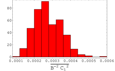
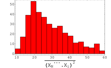
Now let us estimate the decay width for the light moduli. Consider the first benchmark model of -MSSM [39] for example, assuming the weighed dot products take their average value, we find , and . To summarize, the main channels of interest for light moduli decays and their partial widths are , , and . The total width is the sum of these partial width. LSPs arise mainly from gauginos (including LSPs), and , so the LSP branching ratio is the sum of the gaugino and squark channels divided by the total width. One can see that the decay to higgs and scalar dominate the decay of the light moduli. The total decay width is about or the corresponding . The branching ratio of the light moduli to LSP is about . These results should still be roughly correct for other benchmarks, differing at most by since the dependence on the mass spectrum is mild as seen from the explicit result of . The main uncertainty arises from the deviation of those weighted dot products from their typical values. To explore the more general case, one can relax the condition that all the weighted dot products are equal. Instead we choose:
| (146) | |||
| (147) |
Then we vary and according to the distributions of the weighted dot products in Fig.4. The distribution for and the branching ratio to LSPs is shown in Fig.5. One can see that the branching ratio has a very small variation, but the distribution of has a long tail. In the paper, we will use for concreteness, although other values may be possible.
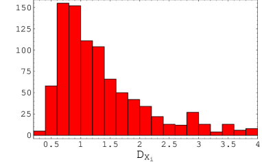
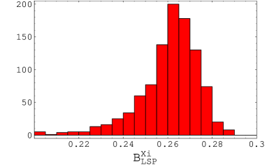
For the heavy modulus , the total decay width is
| (148) |
where corresponds to the decay to gauge bosons , gauginos and higgs bosons, and are given by
| (149) | |||||
| (150) | |||||
| (151) |
In the above result, we have not included the contributions from the decay to non-higgs scalars and fermions since they are suppressed by and given the large mass of the heavy modulus . Taking benchmark 1 of -MSSM in [39] and typical values for weighted dot products, we get , and . The total width is about or the corresponding . The branching ratio to LSPs is about .
The decays of moduli to gravitinos is also very important. The decay of a modulus to gravitinos can be calculated using the following formula: [19]
| (152) |
where is the effective coupling of the modulus field to gravitinos which includes effects of moduli mixing. For the heavy modulus, the coupling arises from the mixing with meson field, since the goldstino is mainly the fermionic partner of the meson. Since the heavy modulus is much heavier than the meson a rough estimate181818There could be an additional suppression in special cases as discussed in [12, 7]. We thank Fuminobu Takahashi for discussions regarding this point. gives . Therefore, for the heavy modulus, the decay rate to gravitino is
| (153) |
This corresponds to . In addition, since the heavy modulus decays much earlier than other moduli, the gravitino produced will be diluted by the subsequent moduli decays. So this estimate is enough for our discussion of gravitino problem. For both the light moduli and the meson fields, the decay to gravitino is kinematically suppressed since .
B.5 Decay Width of the Meson
The total decay width of meson modulus is:
| (154) |
where corresponds to the decay to gauginos , non-higgs scalar and light higgs bosons , and are given by:
| (155) | |||||
| (156) | |||||
| (157) | |||||
Here, as discussed in the last subsection, the low scale couplings to third-generation squarks are dominantly generated from RG running and are related to the coupling by a factor . For the first benchmark of -MSSM in [39] and taking the simplest assumption , we get , and . One can see that this result is enhanced from the naive estimate by the total number of moduli and large (hidden-sector) three-cycle volume . The total decay width is about , corresponding to . The branching ratio to LSPs is about . Again, this can change by for other benchmarks.
References
- [1] G. D. Coughlan, W. Fischler, E. W. Kolb, S. Raby and G. G. Ross, “Cosmological Problems For The Polonyi Potential,” Phys. Lett. B 131, 59 (1983).
- [2] J. R. Ellis, D. V. Nanopoulos and M. Quiros, “On the Axion, Dilaton, Polonyi, Gravitino and Shadow Matter Problems in Supergravity and Superstring Models,” Phys. Lett. B 174, 176 (1986).
- [3] B. de Carlos, J. A. Casas, F. Quevedo and E. Roulet, “Model independent properties and cosmological implications of the dilaton and moduli sectors of 4-d strings,” Phys. Lett. B 318, 447 (1993) [arXiv:hep-ph/9308325].
- [4] T. Banks, D. B. Kaplan and A. E. Nelson, “Cosmological implications of dynamical supersymmetry breaking,” Phys. Rev. D 49, 779 (1994) [arXiv:hep-ph/9308292].
- [5] S. Nakamura and M. Yamaguchi, “A Note on Polonyi Problem,” Phys. Lett. B 655, 167 (2007) [arXiv:0707.4538 [hep-ph]].
- [6] M. Y. Khlopov and A. D. Linde, “Is It Easy To Save The Gravitino?,” Phys. Lett. B 138, 265 (1984).
- [7] M. Dine, R. Kitano, A. Morisse and Y. Shirman, “Moduli decays and gravitinos,” Phys. Rev. D 73, 123518 (2006) [arXiv:hep-ph/0604140].
- [8] M. Endo, M. Kawasaki, F. Takahashi and T. T. Yanagida, “Inflaton decay through supergravity effects,” Phys. Lett. B 642, 518 (2006) [arXiv:hep-ph/0607170].
- [9] V. S. Rychkov and A. Strumia, “Thermal production of gravitinos,” Phys. Rev. D 75, 075011 (2007) [arXiv:hep-ph/0701104].
- [10] M. Endo, K. Hamaguchi and F. Takahashi, “Moduli-induced gravitino problem,” Phys. Rev. Lett. 96, 211301 (2006) [arXiv:hep-ph/0602061].
- [11] S. Nakamura and M. Yamaguchi, “Gravitino production from heavy moduli decay and cosmological moduli problem revived,” Phys. Lett. B 638, 389 (2006) [arXiv:hep-ph/0602081].
- [12] M. Endo, K. Hamaguchi and F. Takahashi, “Moduli / inflaton mixing with supersymmetry breaking field,” Phys. Rev. D 74, 023531 (2006) [arXiv:hep-ph/0605091].
- [13] M. Endo, F. Takahashi and T. T. Yanagida, “Anomaly-Induced Inflaton Decay and Gravitino-Overproduction Problem,” Phys. Lett. B 658, 236 (2008) [arXiv:hep-ph/0701042];
- [14] M. Endo, F. Takahashi and T. T. Yanagida, “Inflaton Decay in Supergravity,” Phys. Rev. D 76, 083509 (2007) [arXiv:0706.0986 [hep-ph]].
- [15] K. Ichikawa, M. Kawasaki and F. Takahashi, “The oscillation effects on thermalization of the neutrinos in the universe with low reheating temperature,” Phys. Rev. D 72, 043522 (2005) [arXiv:astro-ph/0505395].
- [16] S. Nakamura and M. Yamaguchi, “Gravitino production from heavy moduli decay and cosmological moduli problem revived,” Phys. Lett. B 638, 389 (2006) [arXiv:hep-ph/0602081].
- [17] T. Asaka, S. Nakamura and M. Yamaguchi, “Gravitinos from heavy scalar decay,” Phys. Rev. D 74, 023520 (2006) [arXiv:hep-ph/0604132].
- [18] M. Endo, K. Hamaguchi and F. Takahashi, “Moduli-induced gravitino problem,” Phys. Rev. Lett. 96, 211301 (2006) [arXiv:hep-ph/0602061].
- [19] M. Kawasaki, F. Takahashi and T. T. Yanagida, “The gravitino overproduction problem in inflationary universe,” Phys. Rev. D 74, 043519 (2006) [arXiv:hep-ph/0605297].
- [20] M. Nagai and K. Nakayama, “Nonthermal dark matter in mirage mediation,” Phys. Rev. D 76, 123501 (2007) [arXiv:0709.3918 [hep-ph]].
- [21] M. Endo and F. Takahashi, “Non-thermal production of dark matter from late-decaying scalar field at intermediate scale,” Phys. Rev. D 74, 063502 (2006) [arXiv:hep-ph/0606075].
- [22] M. Kawasaki and K. Nakayama, “Baryon Asymmetry in Heavy Moduli Scenario,” Phys. Rev. D 76, 043502 (2007) [arXiv:0705.0079 [hep-ph]].
- [23] S. Kachru, R. Kallosh, A. Linde and S. P. Trivedi, “De Sitter vacua in string theory,” Phys. Rev. D 68, 046005 (2003) [arXiv:hep-th/0301240].
- [24] V. Balasubramanian, P. Berglund, J. P. Conlon and F. Quevedo, “Systematics of moduli stabilisation in Calabi-Yau flux compactifications,” JHEP 0503, 007 (2005) [arXiv:hep-th/0502058].
- [25] J. P. Conlon, F. Quevedo and K. Suruliz, “Large-volume flux compactifications: Moduli spectrum and D3/D7 soft supersymmetry breaking,” JHEP 0508, 007 (2005) [arXiv:hep-th/0505076].
- [26] M. R. Douglas and S. Kachru, “Flux compactification,” Rev. Mod. Phys. 79, 733 (2007) [arXiv:hep-th/0610102].
- [27] M. P. Hertzberg, M. Tegmark, S. Kachru, J. Shelton and O. Ozcan, “Searching for Inflation in Simple String Theory Models: An Astrophysical Perspective,” Phys. Rev. D 76, 103521 (2007) [arXiv:0709.0002 [astro-ph]].
- [28] L. McAllister and E. Silverstein, “String Cosmology: A Review,” Gen. Rel. Grav. 40, 565 (2008) [arXiv:0710.2951 [hep-th]].
- [29] J. P. Conlon and F. Quevedo, “Astrophysical and Cosmological Implications of Large Volume String Compactifications,” JCAP 0708, 019 (2007) [arXiv:0705.3460 [hep-ph]].
- [30] B. Acharya, “A Moduli Fixing Mechanism in theory” arXiv:hep-th/0212294
- [31] C. Beasley and E. Witten, “A note on fluxes and superpotentials in M-theory compactifications on manifolds of G(2) holonomy,” JHEP 0207, 046 (2002) [arXiv:hep-th/0203061].
- [32] B. Acharya and E. Witten, “Chiral fermions from manifolds of G(2) holonomy,” arXiv:hep-th/0109152.
- [33] E. Witten, “Anomaly cancellation on G(2) manifolds,” arXiv:hep-th/0108165.
- [34] M. Atiyah and E. Witten, “M-theory dynamics on a manifold of G(2) holonomy,” Adv. Theor. Math. Phys. 6, 1 (2003) [arXiv:hep-th/0107177].
- [35] E. Witten, “Deconstruction, G(2) holonomy, and doublet-triplet splitting,” arXiv:hep-ph/0201018.
- [36] T. Friedmann and E. Witten, “Unification scale, proton decay, and manifolds of G(2) holonomy,” Adv. Theor. Math. Phys. 7, 577 (2003) [arXiv:hep-th/0211269].
- [37] B. Acharya, K. Bobkov, G. Kane, P. Kumar and D. Vaman, “An M theory solution to the hierarchy problem,” Phys. Rev. Lett. 97, 191601 (2006) [arXiv:hep-th/0606262].
- [38] B. S. Acharya, K. Bobkov, G. L. Kane, P. Kumar and J. Shao, “Explaining the electroweak scale and stabilizing moduli in M theory,” Phys. Rev. D 76, 126010 (2007) [arXiv:hep-th/0701034].
- [39] B. S. Acharya, K. Bobkov, G. L. Kane, J. Shao and P. Kumar, “The -MSSM - An Theory motivated model of Particle Physics,” arXiv:0801.0478 [hep-ph].
- [40] T. Moroi and L. Randall, “Wino cold dark matter from anomaly-mediated SUSY breaking,” Nucl. Phys. B 570, 455 (2000) [arXiv:hep-ph/9906527].
- [41] M. Dine, L. Randall and S. D. Thomas, “Baryogenesis From Flat Directions Of The Supersymmetric Standard Model,” Nucl. Phys. B 458, 291 (1996) [arXiv:hep-ph/9507453].
- [42] N. Kaloper and K. A. Olive, “Dilatons in string cosmology,” Astropart. Phys. 1, 185 (1993).
- [43] R. Brustein, S. P. de Alwis and P. Martens, “Cosmological stabilization of moduli with steep potentials,” Phys. Rev. D 70, 126012 (2004) [arXiv:hep-th/0408160].
- [44] R. Brustein and R. Madden, “Classical corrections in string cosmology,” JHEP 9907, 006 (1999) [arXiv:hep-th/9901044].
- [45] G. Huey, P. J. Steinhardt, B. A. Ovrut and D. Waldram, “A cosmological mechanism for stabilizing moduli,” Phys. Lett. B 476, 379 (2000) [arXiv:hep-th/0001112].
- [46] N. Kaloper, J. Rahmfeld and L. Sorbo, “Moduli entrapment with primordial black holes,” Phys. Lett. B 606, 234 (2005) [arXiv:hep-th/0409226].
- [47] T. Battefeld and S. Watson, “String gas cosmology,” Rev. Mod. Phys. 78, 435 (2006) [arXiv:hep-th/0510022].
- [48] S. Cremonini and S. Watson, “Dilaton dynamics from production of tensionless membranes,” Phys. Rev. D 73, 086007 (2006) [arXiv:hep-th/0601082].
- [49] L. Kofman, A. Linde, X. Liu, A. Maloney, L. McAllister and E. Silverstein, “Beauty is attractive: Moduli trapping at enhanced symmetry points,” JHEP 0405, 030 (2004) [arXiv:hep-th/0403001].
- [50] S. Watson, “Moduli stabilization with the string Higgs effect,” Phys. Rev. D 70, 066005 (2004) [arXiv:hep-th/0404177].
- [51] B. Greene, S. Judes, J. Levin, S. Watson and A. Weltman, “Cosmological Moduli Dynamics,” JHEP 0707, 060 (2007) [arXiv:hep-th/0702220].
- [52] M. Dine, Y. Nir and Y. Shadmi, “Enhanced symmetries and the ground state of string theory,” Phys. Lett. B 438, 61 (1998) [arXiv:hep-th/9806124].
- [53] C. Vafa, “The string landscape and the swampland,” arXiv:hep-th/0509212.
- [54] R. Brustein and P. J. Steinhardt, “Challenges for superstring cosmology,” Phys. Lett. B 302, 196 (1993) [arXiv:hep-th/9212049].
- [55] M. Dine and N. Seiberg, “Is The Superstring Weakly Coupled?,” Phys. Lett. B 162, 299 (1985).
- [56] E. W. Kolb and M. S. Turner, “The Early universe,” Front. Phys. 69, 1 (1990).
- [57] M. Kawasaki, K. Kohri and N. Sugiyama, “Cosmological Constraints on Late-time Entropy Production,” Phys. Rev. Lett. 82, 4168 (1999) [arXiv:astro-ph/9811437].
- [58] G. F. Giudice, E. W. Kolb and A. Riotto, “Largest temperature of the radiation era and its cosmological implications,” Phys. Rev. D 64, 023508 (2001) [arXiv:hep-ph/0005123].
- [59] M. Kawasaki, K. Kohri and N. Sugiyama, “MeV-scale reheating temperature and thermalization of neutrino background,” Phys. Rev. D 62, 023506 (2000) [arXiv:astro-ph/0002127].
- [60] S. Hannestad, “What is the lowest possible reheating temperature?,” Phys. Rev. D 70, 043506 (2004) [arXiv:astro-ph/0403291].
- [61] E. Komatsu et al. [WMAP Collaboration], “Five-Year Wilkinson Microwave Anisotropy Probe (WMAP) Observations:Cosmological Interpretation,” arXiv:0803.0547 [astro-ph].
- [62] I. Affleck and M. Dine, Nucl. Phys. B 249, 361 (1985).
- [63] J. Simon, R. Jimenez, L. Verde, P. Berglund and V. Balasubramanian, “Using cosmology to constrain the topology of hidden dimensions,” arXiv:astro-ph/0605371.
- [64] V. Balasubramanian, P. Berglund, R. Jimenez, J. Simon and L. Verde, “Topology from Cosmology,” arXiv:0712.1815 [hep-th].
- [65] N. Arkani-Hamed, G. L. Kane, J. Thaler and L. T. Wang, “Supersymmetry and the LHC inverse problem,” JHEP 0608, 070 (2006) [arXiv:hep-ph/0512190].