Spin Lifetimes in Quantum Dots from Noise Measurements

Abstract

We present a method of obtaining information about spin lifetimes in quantum dots from measurements of electrical transport. The dot is under resonant microwave irradiation and at temperatures comparable to or larger than the Zeeman energy. We find that the ratio of the spin coherence times $T_{1}/T_{2}$ can be deduced from a measurement of current through the quantum dot as a function the applied magnetic field. We calculate the noise power spectrum of the dot current and show that a dip occurs at the Rabi frequency with a line width given by $1/T_{1}+1/T_{2}$.

Electron spins are promising candidates for qubits (Loss and DiVincenzo, 1998). They constitute a natural two level system but in contrast with nuclear spins they can be highly polarized simply by using routinely available temperature and magnetic field conditions. Additionally one can exploit the mobility of electrons, allowing spin manipulation and measurement via charge currents, e.g. through tunnel barriers.

For applications in quantum information processing it is essential that spins retain phase information for as long as possible. This is usually quantified by the spin coherence time $T_{2}$. Single spin $T_{2}$ times have been determined optically (Hanson et al., 2006; Jelezko et al., 2004) and electrically (Koppens et al., 2006; Petta et al., 2005). Petta et al. (Petta et al., 2005) encoded a qubit in the singlet and triplet states of two electron on a double quantum dot and demonstrated coherent manipulation, while Koppens et al. (Koppens et al., 2006) used pulsed microwaves and top gates to demonstrate coherent oscillations of a single spin in a double dot.

A method for determining spin coherence times using electrical transport through a quantum dot in the stationary state has been suggested by Engel and Loss (Engel and Loss, 2002), but this method can only determine coherence times up to an upper limit that is related to the temperature of the contacts. The study of current-current correlations has emerged as a tool to detect coherence properties of quantum systems such as quantum dots (Zhang et al., 2007). In nanomechanical resonators the noise power spectrum has been used to determine the oscillator occupation number and quality factor (LaHaye et al., 2004; Flowers-Jacobs et al., 2007; Brown et al., 2007). The noise power spectrum of a current interacting with a charge qubit (Barrett and Stace, 2006; Aguado and Brandes, 2004; Korotkov and Averin, 2001; Shnirman et al., 2004) and the current through a quantum dot under microwave radiation have been thoroughly analyzed (Martin et al., 2003; Zhang et al., 2003; Dong et al., 2005).

In this Letter we suggest a method for measuring spin lifetimes using current-current correlations. At experimentally accessible combinations of temperature and magnetic field, where the Zeeman splitting is comparable with or larger than the thermal energy, the measurement of arbitrary intrinsic spin lifetimes becomes possible. To be able to detect the influence of the finite electron spin lifetime on electronic transport through the dot, the dwell time of an electron on the dot has to be comparable to or longer than the spin relaxation times we wish to detect, e.g. through a suitable choice of tunnel barriers. We will henceforth assume this to be the case.

Our model consists of a quantum dot coupled weakly to two leads. The full Hamiltonian after a rotating wave approximation reads $H=H_{D}+H_{E}+H_{T},$ where $H_{D}$ is the Hamiltonian of the dot, $H_{E}$ the Hamiltonian for the leads and $H_{T}$ describes the tunneling between the leads and the dot.

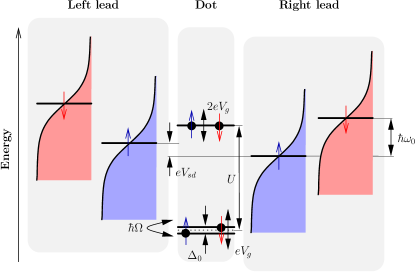
Figure 1: (Color online) The level configuration on the quantum dot and the distribution functions in the leads. The Fermi level of the electrons in the leads is the same for spin up and spin down, but in the rotating frame the energy of the electrons depends on their spin orientation, and the microwave frequency $\omega_{0}$ determines the difference in energy. Also the energy difference of the single electron states on the dot is reduced in the rotating frame from the Zeeman splitting $\Delta_{z}$ to the detuning $\Delta_{0}$, while the energy of the two electron state is separated from the single electron states by the charging energy $U$. The bias voltage $V_{sd}$ is applied symmetrically. The gate voltage $V_{g}$ shifts the energies of the single electron levels by $eV_{g}$ and the two electron level by $2eV_{g}$. The resonant Rabi frequency $\Omega$ couples spin up and spin down.

We choose to model the quantum dot by including three many body states on the quantum dot: the single electron states for spin up and spin down respectively and a singlet two electron state. We assume that the triplet two-electron states are separated from the singlet state by a gap that is large compared to temperature and bias voltage. We also do not take any additional single electron levels into account. In a magnetic field $B$ only the single electron levels are split by the Zeeman energy $\Delta_{z}=g\mu_{B}B$; the singlet is unaffected. Under microwave irradiation with frequency $\omega_{0}$ and after a rotating wave approximation the Hamiltonian for the dot can thus be written

$$H_{D} = \left(eV_{g}-\frac{\Delta_{0}}{2}\right)n_{\uparrow}+\left(eV_{g}+\frac{\Delta_{0}}{2}\right)n_{\downarrow}$$

$$+Un_{\uparrow}n_{\downarrow}+\frac{\hbar\Omega}{2}\left(d_{\downarrow}^{\dagger}d_{\uparrow}+d_{\uparrow}^{\dagger}d_{\downarrow}\right),$$

where $d_{s}^{\dagger}$ and $d_{s}$, $s=\uparrow,\downarrow$, are the creation and annihilation operator for dot electrons in spin up and spin down state respectively and $n_{s}=d_{s}^{\dagger}d_{s}$. $U$ is the mutual Coulomb repulsion energy between two electrons on the dot, $\Omega$ the resonant Rabi frequency, arising from an oscillating magnetic field in x-direction, e.g. in the electric field node of a microwave cavity, and $\Delta_{0}=\Delta_{z}-\hbar\omega_{0}$ is the detuning of the applied microwave field . We have also included the action of a back gate that shifts the single electron energies by the amount $eV_{g}$ (for the energy level diagram see Fig. 1). The Hamiltonian for the leads is given by

$$H_{E}=\sum_{k\alpha s}\varepsilon_{k\alpha s}c_{k\alpha s}^{\dagger}c_{k\alpha s},$$

where $c_{kas}^{\dagger},c_{kas}$, with $\alpha=L,R$ and $s=\uparrow,\downarrow$, are the operators for the lead electrons with momentum $k$. Tunneling from the leads to the dots is given by

$$H_{T}(t)=\sum_{k\alpha s}t_{\alpha}c_{k\alpha s}^{\dagger}(t)d_{s}+h.c.,$$

where $t_{a}$ are the tunneling amplitudes, which in the following we assume to be independent of the electron energy and equal for both leads. We have included the time dependence resulting from the transformation to the rotating frame in the lead operators, introducing $c_{k\alpha\uparrow}^{\dagger}(t)=c_{k\alpha\uparrow}^{\dagger}e^{-i\omega_{0}t}$ and $c_{k\alpha\downarrow}^{\dagger}(t)=c_{k\alpha\downarrow}^{\dagger}e^{i\omega_{0}t}$.

To describe electronic transport through the dot we adapt a Markovian master equation approach (Wabnig et al., 2005). The reduced density matrix of the dot is defined as $\rho(t)=\textnormal{Tr}_{E}\,\left[R(t)\right]$, where $\textnormal{Tr}_{E}\left[\ldots\right]$ denotes the trace over the environment and $R$ is the the density matrix of the full system. Its evolution is given by the master equation

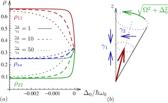
Figure 2: (Color online) (a) The diagonal elements of the density matrix in the energy basis as a function of the detuning for different ratios of the decay rates $\gamma_{2}/\gamma_{1}$ and $\gamma_{e}=10^{-7}\omega_{0}$, $\gamma_{1}=10^{-6}\omega_{0}$, $\Omega=10^{-4}\omega_{0}$, $k_{B}T=\hbar\omega_{0}$, $eV_{sd}=\hbar\omega_{0}$ and $V_{g}=0$. The dotted lines correspond to $\gamma_{2}/\gamma_{1}=50$, the dashed to $\gamma_{2}/\gamma_{1}=10$ and the solid lines to $\gamma_{2}/\gamma_{1}=1$. (b) Diagram illustrating the influence of the different decoherence mechanisms on the spin dynamics.

$d\rho(t)/dt=\mathcal{K}\cdot\rho(t),$ where the super-operator $\mathcal{K}$ consists of three parts: $\mathcal{K}=\mathcal{K}_{0}+\mathcal{K}_{e}+\mathcal{K}_{int}.$ The part describing the free evolution is given by

$$\mathcal{K}_{0}\cdot X=-i\hbar\left[H_{D},X\right],$$

where $X$ can be any operator. Renormalization effects due to interaction with the environment are included in the free evolution (see (Wabnig et al., 2005)). We can also define the free propagator in Fourier space

$$\mathcal{U}_{0}(\varepsilon)=\int dt\,e^{\mathcal{K}_{0}t}\,e^{i\varepsilon t/\hbar}.$$

The influence of the electrons tunneling from the leads is described by the super-operator

$$\mathcal{K}_{e} = \gamma_{e}\int d\varepsilon\sum_{\alpha sij}s_{ij}\left[g^{ij}(\varepsilon-\mu_{\alpha s})\mathcal{A}_{s}^{(i)\dagger}\cdot\mathcal{U}_{0}(\varepsilon)\cdot\mathcal{A}_{s}^{(j)}\right.$$

$$+\left.g^{ij}(\varepsilon+\mu_{\alpha s})\mathcal{A}_{s}^{(i)}\cdot\mathcal{U}_{0}(\varepsilon)\cdot\mathcal{A}_{s}^{(j)\dagger}\right]$$

where $\gamma_{e}=2\pi g(E_{F})\left|t_{L}\right|^{2}$, $g(E_{F})$ being the density of states at the Fermi energy, $s_{ij}=1$ for $i=j$ and $s_{ij}=-1$ otherwise. $\mu_{L/R,\uparrow/\downarrow}=\mu_{L/R}\mp\hbar\omega_{0}/2$, $\mu_{L/R}=\mu\pm eV_{sd}/2$, $g^{11}(\varepsilon)=g^{12}(\varepsilon)=1-f(\varepsilon)$, $g^{21}(\varepsilon)=g^{22}(\varepsilon)=f(\varepsilon)$, $f(\varepsilon)$being the Fermi function, $\mathcal{A}_{s}^{(1)}\cdot X=d_{s}X$ and $\mathcal{A}_{s}^{(2)}\cdot X=Xd_{s}$, and similarly for the hermitian conjugate. The use of the free propagator instead of the self consistent inclusion of the full propagator does not alter the result as long as the distribution functions $g^{ij}$ are smooth on the scale where the full propagator is peaked. In addition to tunneling, we include a phenomenological description of the intrinsic spin decay, given by

$$\mathcal{K}_{int}=\mathcal{K}_{int}^{(1)}+\mathcal{K}_{int}^{(2)}.$$

The first part describes an energy relaxation process leading towards thermal equilibrium $\mathcal{K}_{int}^{(1)}\cdot X=\gamma_{+}\left(\sigma_{+}\sigma_{-}X+X\sigma_{+}\sigma_{-}-\sigma_{+}X\sigma_{-}\right)+\gamma_{-}\left(\sigma_{-}\sigma_{+}X+X\sigma_{-}\sigma_{+}-\sigma_{-}X\sigma_{+}\right)$ with $\gamma_{+}+\gamma_{-}=\gamma_{1}=1/T_{1}$ and $\gamma_{+}/\gamma_{-}=\exp(\Delta_{z}/k_{B}T)$ where $\sigma_{+}=d_{\downarrow}^{\dagger}d_{\uparrow}$, $\sigma_{-}=d_{\uparrow}^{\dagger}d_{\downarrow}$ and $\sigma_{z}=d_{\downarrow}^{\dagger}d_{\downarrow}-d_{\uparrow}^{\dagger}d_{\uparrow}$. The second part is a pure dephasing process $\mathcal{K}_{int}^{(2)}\cdot X=\left(\gamma_{2}-\gamma_{1}/2\right)\left(X-\sigma_{z}X\sigma_{z}\right),$ where $\gamma_{2}=1/T_{2}$. We will be interested in the electronic transport through the dot in the stationary state. The stationary state density matrix can be derived from $\mathcal{K}\cdot\rho_{st}=0.$ This equation was solved analytically using Mathematica. For small detunings $|\Delta_{0}|\ll\hbar\omega_{0}$ and $\hbar\omega_{0}<k_{B}T$ the density matrix elements in the energy basis have the following approximate dependence on the detuning

$$\rho_{ii}(\Delta_{0})=\left\langle i\right|\rho_{st}\left|i\right\rangle=\frac{\rho_{ii}^{(\infty)}\Delta_{0}^{2}+\rho_{ii}^{(0)}\Omega^{2}\gamma_{2}/\gamma_{1}}{\Delta_{0}^{2}+\Omega^{2}\gamma_{2}/\gamma_{1}},$$ (1)

where $\rho_{ii}^{(\infty)}$ denotes the density matrix element far away from resonance and $\rho_{ii}^{(0)}$ the density matrix element on resonance. The dependence of the density matrix elements on the magnetic field for $V_{g}=0$ is shown in Fig. 2(a). Far off resonance the ratio between the spin up and spin down populations is thermal while on resonance the three populations equalize. The width of the transition from the thermal state to the equalized state is given by $\Omega\sqrt{\gamma_{2}/\gamma_{1}}$. This can be understood with the help of Fig. 2(b): The spin precesses around the direction of the effective magnetic field, $\mathbf{B}/g\mu_{B}=(\Omega,0,\Delta_{0})$. For the parts of the precession closer to the z-axis the $\gamma_{1}$ processes drive the spin towards a thermal state along the z-axis of the Bloch sphere. Further away from the z-axis the $\gamma_{2}$ processes dominate, tending to reduce the x and y component to zero. The precession mixes both processes and the relative rates of both relaxation processes determines the stationary state. For $\gamma_{2}>\gamma_{1}$ the spin reacts to a different direction in the magnetic field further from resonance, resulting in a wider transition from thermal to equalized population.

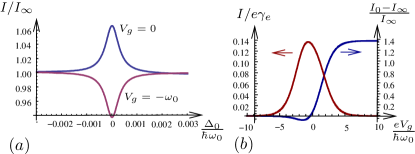
Figure 3: (Color online) (a) The current $I$ as a function of the detuning relative to the current at $\Delta_{0}=0$ without microwave irradiation for different gate voltages and $eV_{sd}=\hbar\omega_{0}$, $k_{B}T=\hbar\omega_{0}$, $\Omega=10^{-4}\omega_{0}$, $\gamma_{e}=10^{-7}\omega_{0}$, $\gamma_{1}=\gamma_{2}=10^{-6}\omega_{0}$. When the magnetic field matches the microwave frequency the current shows a peak or a dip depending on the applied gate voltage. (b) The current at resonance, $I_{0}$, relative to the current without microwave irradiation and the current as a function of the gate voltage, otherwise same values as in (a).

The current through the dot in the stationary state can be expressed as $I=e\textnormal{Tr}_{D}\left[\mathcal{J}\cdot\rho_{st}\right],$ where $\textnormal{Tr}_{D}\left[\ldots\right]$ denotes the trace over the dot degrees of freedom, with the current super-operator given by

$$\mathcal{J} = \gamma_{e}\int d\varepsilon\sum_{\alpha s}\left[g^{ij}(\varepsilon-\mu_{\alpha s})\mathcal{A}_{\alpha s}^{(j)\dagger}\cdot\mathcal{U}_{0}(\varepsilon)\cdot\mathcal{A}_{\alpha s}^{(i)}\right.$$

$$-\left.g^{ji}(\varepsilon+\mu_{\alpha s})\mathcal{A}_{\alpha s}^{(j)}\cdot\mathcal{U}_{0}(\varepsilon)\cdot\mathcal{A}_{\alpha s}^{(i)\dagger}\right],\,i\neq j,\,i,j=1,2.$$

For equal tunneling rates for both leads it is sufficient to consider only the current through one of the tunneling contacts (L or R). In the region of small detunings, $|\Delta_{0}|\ll V_{sd},\,T$, the current can be written approximately as $I=i_{11}\rho_{11}+i_{22}\rho_{22}+i_{33}\rho_{33},$ where the currents $i_{kk},\,k=1,2,3$ depend on $V_{sd},\,V_{g},\,T$ but only weakly on the detuning. The magnetic field dependence of the stationary current for different gate voltages is shown in Fig. 3. Close to the resonance the current shows a peak or a dip, depending on the bias voltage. The dependence of the current on the detuning follows from the detuning dependence of the density matrix elements as

$$I=\frac{I_{\infty}\Delta_{0}^{2}+I_{0}\Omega^{2}\gamma_{2}/\gamma_{1}}{\Delta_{0}^{2}+\Omega^{2}\gamma_{2}/\gamma_{1}},$$

where $I_{\infty}$ is the current far away from the resonance and $I_{0}$ the current at resonance. It is therefore possible to extract the ratio of the dephasing rates $\gamma_{1}/\gamma_{2}$ from the width of the current peak if the Rabi frequency $\Omega$ is known.

The noise power spectrum consists of a constant noise floor, $S_{F}$, and two features, $S_{S}(\omega)$, sitting on top of that noise floor, a peak at zero frequency and a

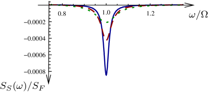
Figure 4: (Color online) The peaked part of noise power spectrum, $S_{S}(\omega)$, relative to the noise floor around the Rabi frequency at resonance ($\Delta_{z}=\hbar\omega_{0})$ and for different rates $\gamma_{1}$ and $V_{g}=0$ , $eV_{sd}=\hbar\omega_{0}$, $k_{B}T=\hbar\omega_{0}$, $\Omega=10^{-4}\omega_{0}$, $\gamma_{e}=10^{-7}\omega_{0}$ and a fixed ratio $\gamma_{2}/\gamma_{1}=10$. The solid line corresponds to $\gamma_{1}=5\cdot 10^{-7}\omega_{0}$, the dashed line to $\gamma_{1}=10^{-6}\omega_{0}$ and the dotted line to $\gamma_{1}=2\cdot 10^{-6}\omega_{0}$.

dip at the Rabi frequency. A similar noise power spectrum was discussed by Aguado and Brandes for a charge qubit in (Aguado and Brandes, 2004). The floor is given by

$$S_{F}=e^{2}\textnormal{Tr}_{D}\left[\mathcal{D}\cdot\rho_{st}\right],$$

where we introduced the diffusion super-operator

$$\mathcal{D} = \gamma_{e}\int d\varepsilon\sum_{\alpha s}\left[g^{ij}(\varepsilon-\mu_{\alpha s})\mathcal{A}_{\alpha s}^{(j)\dagger}\cdot\mathcal{U}_{0}(\varepsilon)\cdot\mathcal{A}_{\alpha s}^{(i)}\right.$$

$$+\left.g^{ji}(\varepsilon+\mu_{\alpha s})\mathcal{A}_{\alpha s}^{(j)}\cdot\mathcal{U}_{0}(\varepsilon)\cdot\mathcal{A}_{\alpha s}^{(i)\dagger}\right],\,i\neq j,\,i,j=1,2.$$

and the features in the noise power spectrum are described by the term

$$S_{S}(\omega)=\textnormal{Tr}_{D}\left[\delta\mathcal{J}\cdot\mathcal{U}(\omega)\cdot\delta\mathcal{J}\cdot\rho_{st}\right],$$

with $\delta\mathcal{J}=\mathcal{J}-I$ and the evolution super operator

$$\mathcal{U}(\varepsilon)=\int dt\,e^{\mathcal{K}t}\,e^{i\varepsilon t/\hbar}.$$

This frequency dependence of the features in the noise power spectrum can be evaluated at resonance to give in the positive half of the spectrum

$$S_{S}(\omega)=S_{0}\frac{\gamma_{e}^{2}}{\omega^{2}+\gamma_{e}^{2}}-S_{\Omega}\frac{\gamma_{\Omega}^{2}}{\left(\omega-\Omega\right)^{2}+\gamma_{\Omega}^{2}},$$

where $S_{0/\Omega}$ are the peak heights at zero and at the Rabi frequency. The peak and the dip have both a Lorentzian line-shape. The peak at zero frequency stems from elastic processes on the dot, its width is determined solely by the tunneling rate $\gamma_{e}$, while the dip appearing at the Rabi frequency is due to processes involving energy exchange on the dot and its width depends on the average of the two spin decoherence rates, $\gamma_{\Omega}=(\gamma_{1}+\gamma_{2})/2$.

We have now all the ingredients to deduce the spin lifetimes $T_{1}$ and $T_{2}$. We can envisage the following measurement procedure: A scan of the gate voltage without an applied microwave field will produce a series of resonances in the current. Selecting one of the resonances and scanning the magnetic field while applying microwave radiation will give information about the presence of an active spin on the dot and the width of the resulting peak gives the ratio $T_{1}/T_{2}$. Finally adjusting the magnetic field to be exactly on resonance and measuring the noise power spectrum around the Rabi frequency we can obtain $1/T_{1}+1/T_{2}$, thus making it possible to deduce $T_{1}$ and $T_{2}$.

Why is is necessary to measure the current noise spectrum at finite frequency? Engel and Loss showed that measuring only the current through a quantum dot as a function of the gate voltage can already give information about $T_{2}$, but to resolve a certain line-width in the dot the distribution functions of the leads have to be sharper than the line-width of the level under consideration. The typical sharpness of the distribution function is given by temperature. The achievable temperatures in today’s dilution refrigerators of $\sim 10\,\textnormal{mK}$ correspond to a resolvable line-width of $\sim 100\,\textnormal{MHz}$, while values for $T_{1/2}$ in group IV semiconductors correspond to line-widths of $<100\,\textnormal{Hz}$ (Tyryshkin et al., 2006). Our scheme will work even at temperatures high compared to the intrinsic line-widths of the dot levels and works well at temperatures comparable to or larger than the Zeeman splitting of the single electron levels, although for temperatures much larger than the Zeeman splitting signal to noise ratio deteriorates. The method operates in the steady state and no pulsed gates are necessary.

What are the limitations of our method? To detect a certain intrinsic decay rate the tunneling rate has to be smaller than that rate. For expected decay rates of the order of $100\,\textnormal{Hz}$ that would correspond to a current of $0.01\,\textnormal{fA}$. Currents of this magnitude are measurable using electron counting techniques (Lu et al., 2003). At the same time we need to detect the noise power spectrum around the Rabi frequency, typically of the order of MHz. To resolve the peak the charge counting has thus to work at rates of $10\,\textnormal{MHz}$ or higher. Radio frequency (RF) single electron transistors or RF quantum point contacts have been shown to work as charge counters up to 1 GHz and should make such measurements possible.

In our modeling we phenomenologically introduced the spin decay rates as constants. A more detailed analysis of the decoherence mechanisms shows that the coherence time $T_{2}$ will, in principle, depend on the Rabi frequency. Assuming a Markovian bath the decay rate is directly related to the spectral density of the bath at the Rabi frequency. Changing the Rabi frequency by altering the microwave intensity should make it therefore possible to probe the spectral density of the bath. A dependence of the coherence time on microwave intensity has been measured in (Koppens et al., 2006). With this simple model we hope to have shown the usefulness of noise measurements in determining spin lifetimes.