QMUL-PH-08-08
ITP-UU-08/16
SPIN-08/16
Finite Temperature Behaviour of O’KKLT Model
Lilia Anguelovaa and Vincenzo Calòb
aInstitute for Theoretical Physics and Spinoza Institute
Utrecht University, 3508 TD Utrecht, The Netherlands
L.Anguelova@phys.uu.nl
bCenter for Research in String Theory
Department of Physics, Queen Mary, University of London
Mile End Road, London, E1 4NS, UK.
v.calo@qmul.ac.uk
Abstract
We summarize our work on the O’Raifeartaigh uplifted KKLT model at finite temperature. We study the system for parameter values for which the zero temperature potential for the volume modulus has a dS minimum. The temperature-dependent part of the effective potential has a runaway behaviour for one exponent in the superpotential, whereas it can have local minima at finite field vevs for two exponents in the superpotential. However, it turns out that, despite the presence of those minima, the zero temperature dS vacuum is not destabilized by thermal corrections within the whole range of validity of our approximations.
1 Introduction
Moduli stabilization is a major problem on the road to relating string theory compactifications with phenomenology. It stems from the fact that the internal space in purely geometric compactifications can have various deformations, which manifest themselves in the four external dimensions as scalar fields without a potential energy (called moduli). As the 4d effective action depends on those moduli, allowing arbitrary values for the latter leads to a lack of predictability of various 4d parameters (coupling constants) and a huge vacuum degeneracy. To resolve this problem, one has to turn on background fluxes [1, 2] and, in the case of type IIB, also take into account non-perturbative effects. The fluxes generate a superpotential for all geometric moduli in type IIA on CY(3) [3] and for the complex structure moduli in type IIB [2]. So for the latter case, one needs to include also non-perturbative effects [4] (or a combination of perturbative and non-perturbative corrections [5]) in order to stabilize the Kähler moduli.
Type IIB flux compactifications are better understood, compared to the type IIA ones, because there is a class of solutions such that the backreaction of the fluxes on the geometry is entirely encoded into warp factors (as opposed to deforming the initial CY to a non-Kähler manifold).111For a comprehensive review of flux compactfications, see [6]. In this context there is a lot of interest in the KKLT proposal for dS vacua in type IIB with stabilized moduli [4]. However, the uplifting of the original AdS vacuum to dS has turned out to be challenging. Recently it was realized that a natural way to achieve this is provided by using metastable dynamical supersymmetry breaking (MDSB). Namely, by coupling the KKLT sector to an ISS sector222See [9] for more details on the Seiberg dual of SQCD, which is now usually called the ISS model., one obtains a dS vacuum that is a result of spontaneous supersymmetry breaking and so is under control in the effective supergravity description [7, 8].
It was argued in [10] that the essential features of F-term uplifting in the KKLT model due to MDSB can actually be captured by taking the uplifting sector to be simply the O’Raifeartaigh model. The resulting so called O’KKLT model is significantly more tractable than the one with ISS uplifting. It was also pointed out there that considering two exponents in the non-perturbative superpotential, instead of one as in the original KKLT proposal, is beneficial for alleviating the tension between low scale supersymmetry breaking and the standard high scale cosmological inflation. Motivated by this, we studied in [11] the effective potential of the O’KKLT model at finite temperature.
Thermal corrections to a model exhibiting MDSB (more precisely, the ISS model) were first studied in [12, 13]. These works showed that the metastable minimum is thermodynamically preferable compared to the global supersymmetric vacuum. Thus the finite temperature considerations provide a natural mechanism for the system to end up at zero temperature in a local minimum instead of in the global one. The same conclusion holds also upon coupling the ISS model to supergravity [14]. However, understanding the finite temperature behaviour of the full KKLT-ISS model is rather complicated technically.333This problem was studied in the recent work [15]. Investigating the O’KKLT model instead, we are able to compute the one-loop temperature corrections to the effective potential for the volume modulus and study the resulting phase structure of the system.
2 O’KKLT model
The O’KKLT model of [10] is determined by the following Kähler potential and superpotential:
| (2.1) |
where the function is either
| (2.2) |
In other words, this is the combination of the KKLT model (with volume modulus ) and the O’Raifeartaigh model. In fact, the latter is considered in the regime in which the two heavy scalar fields are integrated out and one is left with a single field, . The last term in comes from the leading one-loop correction in an expansion in , where and are the remaining couplings in the full O’Raifeartaigh superpotential: . The parameter in denotes a particular combination of couplings, namely with being a numerical constant of order 1. Also, we assume and consider the field space region where (we work in units ). For more details, see [10, 11]. We will study the effective model given by (2.1)-(2.2), regardless of any underlying microphysics.
At zero temperature the KKLT model alone has one or two AdS vacua, depending on whether there are one or two exponents in , that are situated at finite values of . The O’Raifeartaigh model uplifts one of this minima to dS.444Clearly, the Dine-Seiberg minimum at infinity is also present. Our goal is to study the phase structure of the theory (2.1) at finite temperature in order to answer the question whether the fields roll towards the dS vacuum upon cooling down.
3 Effective potential at finite temperature
We will compute the one-loop finite temperature effective potential for the O’KKLT model. Let us begin by recalling the general expression for a field theory of a set of fields . It was derived first for a renormalizable theory in [18], using the zero-temperature functional integral method of [19], and later generalized to supergravty in [16]. Namely, the effective potential is a function of the background values of the fields , which to one-loop order is given by:
| (3.1) |
Here is the standard classical supergravity expression:
| (3.2) |
is the zero temperature one-loop contribution, encoded in the Coleman-Weinberg formula, and finally the temperature-dependent correction is:
| (3.3) |
In the above formula, and denote the traces over the mass matrices of the scalar and fermion fields respectively in the classical background 555In (3.3), is computed summing over Weyl fermions., which are given by [17]:
| (3.4) |
with being the same as in (3.2) and
| (3.5) |
where . The constants and in (3.3) are the total numbers of bosonic and fermionic degrees of freedom. Since we will only need the derivatives of w.r.t. some , we will drop from now on the piece of the effective potential. Also, for convenience, we will denote the remaining expression in (3.3) just by . Let us also note that the high temperature expansion (3.3) is valid only in the regime, in which all masses are much smaller than the energy scale set by the temperature.
4 Phase structure at finite T
It is usually expected that at high temperature the effective potential is dominated by its temperature-dependent part . So the system under consideration is naturally in a minimum of the latter. As the temperature decreases, a point may be reached at which the system undergoes a second order phase transition and starts rolling towards a different minimum. In order to investigate the details of this picture for the O’KKLT model, we first have to address the question whether there are finite vev minima of the relevant potential . In [11] we show that for in (2.1) the behaviour of is in fact runaway, implying decompactification of the internal space. On the other hand, for the temperature-dependent part can have minima at finite vevs. So in the rest of this section we concentrate on the case of two exponents in the superpotential.
In this case, the potential generically has two minima with finite field vevs. Assuming that the starting point at high temperature is one of those minima (we take the deeper one, which is situated at lower vevs), one can find the critical temperature for a second order phase transition, together with the field space position at which the transition occurs, by solving the system
| (4.1) |
where we have symbolically denoted by ′ and ′′ first and second derivatives with respect to . We want to know whether as a result of this transition the system starts rolling towards the zero-temperature dS vacuum or in the opposite direction.666It turns out that the finite minimum, which is our starting point, is always between the dS and the susy vacua [11]. Let us first note that for a system with symmetry the above equations reduce to the more familiar condition , where is the zero-temperature mass of the field whose nonzero vev characterizes the new vacuum. In our case, however, there is no such simplification and we need to solve the full system (4.1). Unfortunately though, these are transcendental equations that cannot be solved analytically (for more details, see [11]). So we turn to numerical considerations.
Before proceeding further, we have to make a conceptual remark. Clearly, the numerical results will depend on the values of the various parameters in (2.1)-(2.2).777One can take without any loss of generality and then the essential parameters are , , , and [11]. In particular, for some choices of parameters there may be a single minimum of at finite vevs or even no minimum at all (of course, other than the Minkowski one at infinity). This is the same kind of situation as for the zero-temperature potential studied in [10]. Namely, there are many parameter values such that does not have a dS (or even any) minimum. What is important, however, is that there exist many parameter choices for which does have a dS vacuum [10]. These are exactly the parameter values that are relevant for moduli stabilized dS vacua. In the same vein, here we are interested in the sets of parameters for which has at least one finite vevs minimum, when has a dS vacuum, as these are the choices for which one can have a dS compactification that is not destabilized by thermal effects.
We have found several sets of parameters, for which the system is in the desired regime; see Table 1, where .
| -1.040 | 4.88 | 7.84 | 5.62 | |||
| -1.036 | 4.50 | 7.40 | 5.25 | |||
| -1.032 | 4.11 | 6.92 | 4.83 | |||
| -1.028 | 3.73 | 6.44 | 4.44 | |||
| -1.024 | 3.34 | 6.00 | 4.04 | |||
| -1.020 | 2.96 | 5.52 | 3.64 | |||
| -1.016 | 2.55 | 5.02 | 3.20 |
According to this table, the O’KKLT model seems to exhibit the behaviour of interest only at discrete points in parameter space. Strictly speaking, this is only true up to a small variation of one (or more) parameter(s) for some of the sets; for more details see [11]. Nevertheless, it is quite interesting to note that in order to move from one point in parameter space to another, such that at both points one has the same kind of physics, generically one needs to change in a discrete way at least two parameters. This suggests that anthropic arguments of the kind of [20] might be too naive. Recall that in such considerations one usually argues that a particular value of a given constant of nature (for example, the cosmological constant) is anthropically preferred since varying that constant, while keeping all other coupling constants fixed, leads to drastic physics changes. Given the example of the O’KKLT model however, it seems conceivable that these anthropic/environmental arguments might fail under more general variations, i.e. discrete changes of more than one coupling constant at the same time.888However, see [21] for arguments in favor of Weinberg’s argument in the case when both the cosmological constant and the Higgs mass are varied, while the remaining couplings are held fixed. This issue is well-worth investigating in more realistic models.
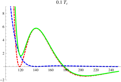
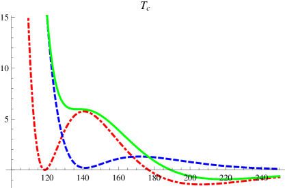
Let us now turn to the question about the occurrence of a second order phase transition. From Table 1 we see that the minimum of interest is situated between the dS and AdS vacua of the zero temperature potential. So it seems meaningful to ask whether the system rolls towards the meatstable or the supersymmetric vacua upon cooling down. However, the critical temperature for the relevant second order phase transition turns out to be always of order ; an example, representative for all rows of Table 1, is illustrated in Figure 1.999For convenience, the graph of (the green continuous line) does not include the term in (3.3); as the latter is field-independent, it only leads to an irrelevant overall shift of the plot. Now, recall that we are working in units of . Hence the critical temperature that we obtain is . This is rather unexpected since the potential barrier between the relevant minima is of order , as can be seen on the figure, and so one would have expected intuitively that . In fact, such a high implies that we cannot reliably conclude that there is a phase transition, since the supergravity approximation is near the threshold of its validity. Furthermore, such is clearly outside of the validity of the single field approximation to the O’Raifeartaigh model.101010Recall that this low-energy effective description of the O’Raifeartaigh model, obtained by integrating out the two heavy fields, is a motivation to consider the model determined by (2.1)-(2.2), although the latter can certainly be studied on its own without viewing it as an approximation to the O’Raifeartaigh model (since neither of the two is supposed to provide a fundamental description anyway). Nevertheless, we can turn this around and conclude that for the whole range of validity of the supergravity approximation, i.e. for , (and hence even more so for the whole range of validity of the single field low-energy approximation to the full O’Raifeartaigh model) the extrema of the effective potential of the system are determined by the zero-temperature part and not by .111111Note that, because of the constant term that we are omitting, this does not mean that the magnitude of itself is determined by . Therefore, at the level of our approximations the de Sitter minimum is not destabilized by thermal effects.
If we take the O’KKLT model as a simple toy model of the early Universe, the behaviour that we have uncovered above implies that reheating does not destabilize the metastable minimum of the zero-temperature potential for the volume modulus . Indeed, at the end of the inflationary stage the Universe is generically expected to be very cold. Hence it will be in a local minimum of .121212Note that the modulus , defined in (3.6), should not be confused with the inflaton field. The exit from inflation comes with the decay of the inflaton into various particles and the resulting reheating of the Universe to some temperature . It is usually expected that and so our considerations can be applied to this system, leading to the conclusion that we stated in the beginning of this paragraph. Namely, we can conclude that reheating does not destabilize the dS vacuum of the volume modulus or, in other words, does not lead to decompactification of the internal space.
This new point of view raises the question whether the zero-temperature dS vacuum could remain a local minimum of the total effective potential even for parameter values for which has a runaway behaviour (of course, within the range of validity of our approximations). It is easy to verify that this is indeed the case for sets of parameters that are small variations of those in Table 1, such that does not have any finite-vev minima while the dS minimum of is preserved. A more detailed study of this issue for a broad range of parameter values merits a separate investigation.
5 One exponential revisited
In light of the results of the previous section, it is worth to re-examine the case of one exponent in the superpotential in order to see whether the zero-temperature dS vacuum can survive at high , despite the runaway behaviour of in this case. Let us, for simplicity, view here the model (2.1) with as an effective description on its own.131313I.e., we will only worry about one cut-off scale - the Planck scale. One can show analytically [11] that the dS minimum of is not washed out by the thermal corrections only when certain order-of-magnitude inequalities are satisfied. In particular, we have found that for the largest allowed values of the parameters and (i.e., the values that require the smallest amount of fine-tuning and are thus the most preferable ones) the dS minimum persists in the total as long as . Clearly then, by taking one can ensure that the dS vacuum is not destabilized by the temperature contribution for the whole range of validity of the supergravity approximation. Obviously, for or smaller this is not the case anymore as temperatures greater than are well within the range and hence one can reliably conclude that at high the internal space decompactifies.
It is interesting to note that the recent work [22] reached the same conclusions, that we did in Sections 4 and 5 here, from a different perspective. Namely, they studied the dynamics of a similar system at finite temperature and showed that the thermal corrections have quite a limited effect on its evolution and that, under certain conditions, one can have temperatures as high as without losing the minimum of the zero-temperature potential, despite the lack of finite vev minima of .
Acknowledgements
L.A. would like to thank the organizers of the 3rd RTN Workshop ”Constituents, Fundamental Forces and Symmetries of the Universe” held in Valencia, October 2007, for the opportunity to present this work. The research of L.A. is supported in part by the EU RTN network MRTN-CT-2004-005104 and INTAS contract 03-51-6346. The work of V.C. is supported by a Queen Mary studentship.
References
- [1] K. Dasgupta, G. Rajesh and S. Sethi, M-theory, Orientifolds and G-flux, JHEP 9908 (1999) 023, hep-th/9908088.
- [2] S. Giddings, S. Kachru and J. Polchinski, Hierarchies from Fluxes in String Compactifications, Phys. Rev. D66 (2002) 106006, hep-th/0105097.
- [3] J.-P. Derendinger, C. Kounnas, P. M. Petropoulos and F. Zwirner, Superpotentials in IIA Compactifications with General Fluxes, Nucl. Phys. B715, (2005) 211, hep-th/0411276; G. Villadoro and F. Zwirner, N=1 Effective Potential from Dual Type-IIA D6/O6 Orientifolds with General Fluxes, JHEP 0506 (2005) 047, hep-th/0503169; O. DeWolfe, A. Giryavets, S. Kachru and W. Taylor, Type IIA Moduli Stabilization, JHEP 0507 (2005) 066, hep-th/0505160.
- [4] S. Kachru, R. Kallosh, A. Linde and S. Trivedi, de Sitter Vacua in String Theory, Phys. Rev. D68 (2003) 046005, hep-th/0301240.
- [5] V. Balasubramanian, P. Berglund, J. Conlon and F. Quevedo, Systematics of Moduli Stabilisation in Calabi-Yau Flux Compactifications, JHEP 0503 (2005) 007, hep-th/0502058; J. Conlon, F. Quevedo and K. Suruliz, Large-Volume Flux Compactifications: Moduli Spectrum and D3/D7 Soft Supersymmetry Breaking, JHEP 0508 (2005) 007, hep-th/0505076.
- [6] M. Graña, Flux Compactifications in String Theory: A Comprehensive Review, Phys. Rept. 423 (2006) 91, hep-th/0509003.
- [7] E. Dudas, C. Papineau and S. Pokorski, Moduli Stabilization and Uplifting with Dynamically Generated F-terms, JHEP 0702 (2007) 028, hep-th/0610297.
- [8] H. Abe, T. Higaki, T. Kobayashi and Y. Omura, Moduli stabilization, F-term uplifting and soft supersymmetry breaking terms, Phys. Rev. D75 (2007) 025019, hep-th/0611024.
- [9] K. Intriligator, N. Seiberg and D. Shih, Dynamical SUSY Breaking in Meta-Stable Vacua, JHEP 0604 (2006) 021, hep-th/0602239.
- [10] R. Kallosh and A. Linde, O’KKLT, JHEP 0702 (2007) 002, hep-th/0611183.
- [11] L. Anguelova and V. Calò, O’KKLT at Finite Temperature, arXiv:0708.4159 [hep-th].
- [12] S. Abel, C. Chu, J. Jaeckel and V. Khoze, SUSY Breaking by a Metastable Ground State: Why the Early Universe Preferred the Non-supersymmetric Vacuum, JHEP 0701 (2007) 089, hep-th/0610334.
- [13] W. Fischler, V. Kaplunovsky, C. Krishnan, L. Mannelli and M. Torres, Meta-Stable Supersymmetry Breaking in a Cooling Universe, JHEP 0703 (2007) 107, hep-th/0611018.
- [14] L. Anguelova, R. Ricci and S. Thomas, Metastable SUSY Breaking and Supergravity at Finite Temperature, Phys. Rev. D77 (2008) 025036, hep-th/0702168.
- [15] C. Papineau, Finite Temperature Behaviour of the ISS-uplifted KKLT Model, arXiv:0802.1861 [hep-th].
- [16] P. Binetruy and M. Gaillard, Temperature Corrections, Supersymmetric Effective Potentials and Inflation, Nucl. Phys. B254 (1985) 388.
- [17] P. Binetruy and M. Gaillard, Temperature Corrections in the Case of Derivative Interactions, Phys. Rev. D32 (1985) 931.
- [18] L. Dolan and R. Jackiw, Symmetry Behavior at Finite Temperature, Phys. Rev. D9 (1974) 3320.
- [19] R. Jackiw, Functional Evaluation of the Effective Potential, Phys. Rev. D9 (1974) 1686.
- [20] S. Weinberg, Anthropic Bound on the Cosmological Constant, Phys. Rev. Lett. 59 (1987) 2607; M. Tegmark and M. Rees, Why is the CMB Fluctuation Level ?, Astrophys. J. 499 (1998) 526, astro-ph/9709058; S. Barr and A. Khan, Anthropic Tuning of the Weak Scale and of in two-Higgs-doublet Models, Phys. Rev. D76 (2007) 045002, hep-ph/0703219.
- [21] N. Arkani-Hamed, S. Dimopoulos and S. Kachru, Predictive Landscapes and New Physics at a TeV, hep-th/0501082.
- [22] T. Barreiro, B. de Carlos, E. Copeland and N. Nunes, Moduli Evolution in the Presence of Thermal Corrections, arXiv:0712.2394 [hep-ph].