Revised bolometric corrections and interstellar extinction coefficients for the ACS and WFPC2 photometric systems

Abstract

We present extensive tables of bolometric corrections and interstellar extinction coefficients for the WFPC2 and ACS (both WFC and HRC) photometric systems. They are derived from synthetic photometry applied to a database of spectral energy distributions covering a large range of effective temperatures, surface gravity, and metal content. Carbon stars are also considered. The zero-points take into consideration the new high-accuracy Vega fluxes from Bohlin. These tables are employed to transform Padova isochrones into WFPC2 and ACS photometric systems using interstellar extinction coefficients on a star-to-star basis. All data are available either in tabular form or via an interactive web interface in the case of the isochrones. Preliminary tables for the WFC3 camera are also included in the database.

1 Introduction

The Advanced Camera for Surveys (ACS) aboard the Hubble Space Telescope (HST) has provided some of the deepest photometric optical images ever taken. At the same time, the Wide Field and Planetary Camera 2 (WFPC2) camera aboard HST has a rich photometric data archive dating back more than a decade. Both cameras have taken many images of galaxies within $\sim$5 Mpc, providing reliable photometry for individual stars within these nearby galaxies. This resolved stellar photometry contains detailed information about the history of star formation and chemical enrichment. Extracting this information requires stellar evolution isochrones that track the photometric properties of stars of different ages and metallicities. Only with precise models can these rich samples of stellar photometry provided by ACS and WFPC2 be translated into coherent histories of star formation and chemical evolution.

Given the extreme importance of the stellar photometric data provided by ACS and WFPC2, many authors have described the conversion from theoretical stellar models into these systems. For the WFPC2 system, transformations and isochrones have been provided by Holtzman et al. (1995), Chiosi et al. (1997), Salasnich et al. (2000), Girardi et al. (2002), Lejeune (2002), and Dotter et al. (2007). For ACS, BC tables and isochrones have been provided at http://pleiadi.oapd.inaf.it since 2003, as an addition to the Girardi et al. (2002) database, and later by Bedin et al. (2005) and Dotter et al. (2007).

With the present paper, our goal is to provide revised and homogeneous tables of BCs and interstellar extinction coefficients in the ACS and WFPC2 systems, updating as much as possible the files distributed by Girardi et al. (2002) in precedence. The motivation for an overall revision of the BC tables reside mainly on the definition of better spectrophotometric standards by Bohlin and collaborators (Bohlin 2007, and references therein), and more complete libraries of stellar spectra, whereas filter transmission curves for these instruments remain essentially the same as in the original papers by the instrument teams. A consistent set of interstellar extinction coefficients for these systems would be particularly important since the unique resolution of HST allows useful optical photometry to be obtained even for heavily reddened regions (with say $A_{V}\gtrsim 3$; see e.g. Recio Blanco et al. 2005), for which interstellar extinction coefficients being used so far may not be accurate enough.

The BC and interstellar extinction tables will be used to transform theoretical isochrones to these systems, and will be extensively applied in the interpretation of ANGST/ANGRRR data.

We proceed as follows: Sect. 2 describes the steps involved in the derivation of bolometric corrections via synthetic photometry, from the assembly of a spectral library to the definition of zeropoints. Sect. 3 describes the interstellar extinction coefficients. The results are used in Sect. 4 to convert theoretical isochrones into the ACS and WFPC2 systems, which are made publicly available. They are briefly illustrated in Sect. 5, by means of a few comparisons with observations.

2 Bolometric corrections

Given the spectral fluxes at the stellar surface, $F_{\lambda}$, bolometric corrections for any set of filter transmission curves $S_{\lambda}$ are given by (see Girardi et al. 2002 for details)

$$BC_{S_{\lambda}} = M_{\rm bol,\odot}-2.5\,\log\left[4\pi(10\,{\rm pc})^{2}F_{\rm bol}/L_{\odot}\right]$$

$$+2.5\,\log\left(\frac{\int_{\lambda_{1}}^{\lambda_{2}}\lambda F_{\lambda}\,10^{-0.4A_{\lambda}}S_{\lambda}\mbox{${\rm d}$}\lambda}{\int_{\lambda_{1}}^{\lambda_{2}}\lambda f^{0}_{\lambda}S_{\lambda}\mbox{${\rm d}$}\lambda}\right)-m_{S_{\lambda}}^{0}$$

where $f^{0}_{\lambda}$ represents a reference spectrum (incident on the Earth’s atmosphere) that produces a known apparent magnitude $m^{0}_{S_{\lambda}}$, $F_{\rm bol}=\int_{0}^{\infty}F_{\lambda}\mbox{${\rm d}$}\lambda=\sigma T_{\rm eff}^{4}$ is the total emerging flux at the stellar surface, and $A_{\lambda}$ is the interstellar extinction curve in magnitude units. Once $BC_{S_{\lambda}}$ are computed, stellar absolute magnitudes follow from

$$M_{S_{\lambda}}=M_{\rm bol}-BC_{S_{\lambda}}\,\,\,,$$ (2)

where

$$M_{\rm bol} = M_{\rm bol,\odot}-2.5\,\log(L/L_{\odot})$$

$$= M_{\rm bol,\odot}-2.5\,\log(4\pi R^{2}F_{\rm bol}/L_{\odot})\,\,\,\,.$$

As in Girardi et al. (2002), we adopt $M_{\rm bol,\odot}=4.77$, and $L_{\odot}=3.844\times 10^{33}\,{\rm erg\,s^{-1}}$ (Bahcall et al. 1995).

Notice that Eq. 2 uses photon count integration instead of energy integration, as appropriate to most modern photometric systems that use photon-counting detectors instead of energy-amplifiers. The equation also includes the interstellar extinction curve $A_{\lambda}$, that will be discussed later in Sect. 3. $A_{\lambda}=0$ is assumed for the moment.

2.1 A library of spectral fluxes

Girardi et al. (2002) assembled a large library of spectral fluxes, covering wide ranges of initial metallicities ([M/H] from $-2.5$ to $+0.5$), $T_{\rm eff}$ (from 500 to 50 000 K), and $\log g$ (from $-2$ to $5$). This grid is wide enough to cover most of the stellar types that constitute the bulk of observed samples in resolved galaxies. The grid is composed of ATLAS9 “NOVER” spectra from Castelli et al (1997, see also Bessell et al. 1998) for most of the stellar types, Allard et al. (2000a) for M, L and T dwarfs, Fluks et al. (1994) empirical spectra for M giants, and finally pure blackbody spectra for stars exceeding 50 000 K. Since then, we have updated part of this library, namely:

1) As part of the TRILEGAL project (Girardi et al. 2005), we have included spectra for DA white dwarfs from Finley et al. (1997) and Homeier et al. (1998) for $T_{\rm eff}$ between 100 000 and 5 000 K.

2) We now use Castelli & Kurucz (2003) ATLAS9 “ODFNEW” spectra, which incorporate several corrections to the atomic and molecular data, especially regarding the molecular lines of CN, OH, SiO, H₂O and TiO, and the inclusion of HI–H⁺ and HI–H⁺ quasi-molecular absorption in the UV. These new models are considerably better than the previous NOVER ones, especially in the UV region of the spectrum, and over most of the wavelength range for $T_{\rm eff}$ between $\sim 4500$ and $3500$ K (see figs. 1 to 3 in Castelli & Kurucz 2003).

3) We have also incorporated in the library the Loidl et al. (2001) spectral fluxes of solar-metallicity carbon (C-) stars derived from static model atmospheres. They are computed for $T_{\rm eff}$ in the range from 2600 to 3600 K, and for C/O$=1.1$ and 1.4. The C/O$=1.1$ spectra are now used for all C/O$>1$ models, replacing the Fluks et al. (1994) spectra of M giants which were previously (and improperly) used for all cool giants including C-rich ones.

Regarding this latter aspect, it is to be noticed that all Padova isochrones published since 2001 (Marigo & Girardi 2001; Cioni et al. 2006; Marigo et al. 2008) do take into consideration the third dredge-up events and hence the conversion to a C-type phase during the TP-AGB evolution. This phase, characterised by the surface C/O$>1$, has to be represented with either proper C-rich spectra, or alternatively, with empirical $T_{\rm eff}$-colour relations as in Marigo et al. (2003). The use of Loidl et al. (2001) spectra frees us definitely from using empirical relations for C stars. Note that such empirical relations would not even be available for the ACS and WFPC2 filters we are interested in. In fact, empirical $T_{\rm eff}$-colour relations for C stars are usually limited to red and near-IR filters, and mainly to $IJHK$.

Although the Loidl et al. (2001) models are quite limited in their coverage of the parameter space of C stars (i.e. [M/H], C/O, $T_{\rm eff}$, and $\log g$) they represent a useful first approach toward obtaining realistic colours for them. Work is in progress to extend significantly the parameter space of such models (Aringer et al., in preparation).

2.2 Filters and zeropoints

As can readily be seen in Eq. 2, in the formalism adopted here, the photometric zeropoints are fully determined by a reference spectral energy distribution $f^{0}_{\lambda}$, which provides a given set of reference magnitudes $m_{S_{\lambda}}^{0}$.

In this work, we adopt the latest Vega spectral energy distribution from Bohlin (2007) as $f^{0}_{\lambda}$. This Vega spectrum represents a great improvement over previous ones distributed and used in the past. It is the result of an effective effort using STIS to provide a set of stellar spectrophotometric standards with an absolute calibration to better than 1 percent at near-UV to blue wavelengths. The best-fitting ATLAS9 model for Vega in this spectral range is then used to complement its spectral energy distribution at red and near-IR wavelengths. From Bohlin (2007), one can conclude the new Vega spectrum is likely accurate to about 1–2 percent over the complete 3200–10000 Å interval.

Having adopted Bohlin’s (2007) Vega spectrum, we have just to specify the Vega magnitudes in ACS and WFPC2 filters to completely define our zeropoints. Following Holtzman et al.’s (1995) definition of the WFPC2 synthetic system, we define that Vega has the same magnitudes in WFPC2 filters as in the Johnson-Cousins filters that are closest to them in wavelength. This choice means a magnitude of 0.02 for all filters from F336W to F450W, 0.03 for F555W and F569W, 0.035 from F606W to F850LP, but for F702W which has magnitude 0.039. For filters blueward of F300W, Vega magnitudes are assumed to be zero.

Then, for ACS we adopt the same definition as Sirianni et al. (2005), that Vega has zero magnitudes in all ACS filters. For a question of completness, we provide tables also for the AB and ST magnitude systems.

These are of course synthetic definitions of WFPC2 and ACS systems, that may present small systematic offsets with respect to the real systems (such as the flight WFPC2 system defined by Holtzman et al. 1995) to which observations are commonly transformed.

Finally, the filter transmission curves $S_{\lambda}$ – including the telescope and camera throughputs – for WFPC2 are created with SYNPHOT/STSDAS v3.7 using the most up-to-date throughput and sensitivity reference files available at January 15, 2008. For WFPC2/F170W and WFPC2/F218W, instead, they are taken from Holtzman et al. (1995). All of the wide filters are considered. ACS filter throughputs are from Sirianni et al. (2005). They are almost identical to those provided by SYNPHOT/STSDAS v3.7.

2.3 Behaviour of bolometric corrections

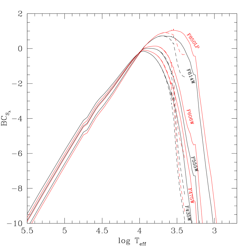
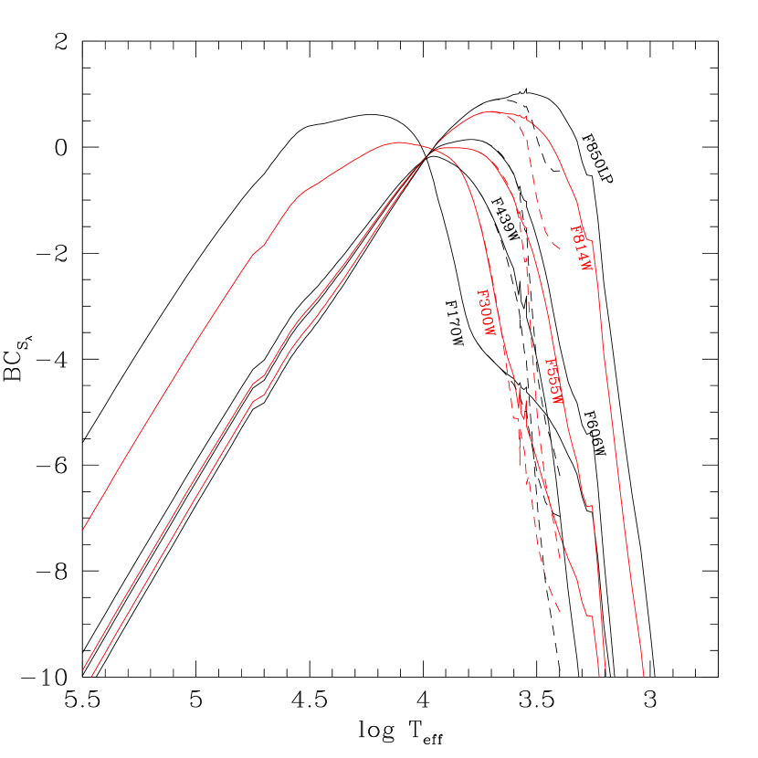
Figure 1: $BC_{S_{\lambda}}$ as a function of $T_{\rm eff}$, for both dwarfs (continuous lines) and giants (dashed lines), for some of the ACS/WFC and WFPC2 filters.

Figure 1 shows how BCs depend on $T_{\rm eff}$ for a series of ACS and WFPC2 filters. In practice, we illustrate it for a sequence of dwarfs of $\log g=5$, and for a sequence of subgiants and giants (of M type at the coolest $T_{\rm eff}$) following the relation $\mbox{$T_{\rm eff}$}=3250+500\,\log g$ (in c.g.s. units), which roughly describes the position of the Hayashi track in the HR diagram of low-mass stars with near-solar metallicity. The central part of the $T_{\rm eff}$ interval reflects the behaviour of ATLAS9 synthetic spectra. The small discontinuities in the figure occur as we change from one spectral library to another, namely:

• The wiggles at $\log\mbox{$T_{\rm eff}$}\simeq 3.54$ occur when we pass from ATLAS9 to Fluks et al. (1994) spectra for M giants, and to Allard et al. (2000a) spectra for M dwarfs.

• The step at $\log\mbox{$T_{\rm eff}$}\simeq 3.27$ occurs when we change between the “AMES” and “AMES-dusty” among Allard et al. (2000a) spectra. The latter include dust formation in the outer atmosphere, and are computed for solar-metallicity only (see Chabrier et al. 2000; Allard et al. 2000b, 2001 for more details).

• A second, less pronounced step at $\log\mbox{$T_{\rm eff}$}\simeq 4.75$ occurs when we start using blackbody spectra instead of ATLAS9.

Among these discontinuities, the most important are the wiggles at $\log\mbox{$T_{\rm eff}$}\simeq 3.54$ because they occur at $T_{\rm eff}$ in which many stars of Local Group galaxies are routinely observed in optical to near-IR passbands. In order to limit the effect of such wiggles in the final isochrones, we adopt a smooth transition between the different sources of BC, for both dwarfs and giants, over the $\log\mbox{$T_{\rm eff}$}$ interval from 3.542 and 3.590. This is the reason why isochrones using these transformations (see the Fig. 5 later for an example) do not present significant discontinuities.

It is also interesting to note, in Fig. 1, the anomalous behaviour of F170W in WFPC2 which for cool stars provides brighter magnitudes than redder filters. This behaviour is a consequence of its red leak (see also Holtzman et al. 1995). A similar effect is also present, but much less pronounced, in the F300W filter.

3 Interstellar extinction coefficients

As already mentioned, Eq. 2 can be used together with an interstellar extintion curve, $A_{\lambda}$, to derive bolometric corrections already including the effect of interstellar extinction. Alternatively, we can derive relative interstellar extinction coefficients, $A_{S_{\lambda}}/A_{V}$, by simply using

$$A_{S_{\lambda}}/A_{V}=[BC_{S_{\lambda}}(0)-BC_{S_{\lambda}}(A_{V})]/A_{V}$$ (4)

where the 0 stands for the $A_{\lambda}=0$ case.

The interstellar extinction curve $A_{\lambda}$ we use in Eq. 2 is taken from Cardelli et al. (1989) with $R_{V}=A_{V}/E_{B\!-\!V}=3.1$, and integrated with the O’Donnell (1994) correction for $909<\lambda/{\rm\AA}<3030$. Other extinction curves and $R_{V}$ values can be easily implemented whenever necessary (e.g. Vanhollebeke et al. 2008). Our calculations are essentially identical to those by Holtzman et al. (1995) and Sirianni et al. (2005), but are now performed for a more extended range of stellar parameters and extinction values.

Before proceeding, it is interesting to note that the two parameters in Cardelli et al. (1989) interstellar extinction curve, $A_{V}$ and $R_{V}$, refer to the Johnson’s $B$ and $V$ bands. However, this does not imply that synthetic realisations of the Johnson system will recover the same values of $R_{V}$ and $A_{V}$ when the extinction curve is applied. As examples, we find that for a G2V star the Bessell (1990) version of the Johnson system provide $A_{V,{\rm Bessell}}=1.006\,A_{V}$ and $R_{V,{\rm Bessell}}=3.457$, whereas Maíz Apellániz (2006) version gives essentially the same numbers, with differences appearing just at the fifth decimal. These numbers change somewhat as a function of spectral type and $A_{V}$ itself (as will be illustrated below for HST systems). Therefore, $A_{V}$ should be considered as just “the parameter that describes the total amount of interstellar extinction in Cardelli et al. (1989) law”, rather than a precise physical measure of the $V$-band extinction. A similar comment applies also to $R_{V}$: in the context of this paper it is “the parameter that describes the shape of the interstellar extinction curve”, rather than the total-to-selective interstellar extinction of Johnson-like systems.

Figure 2: The variation of $A_{S_{\lambda}}/A_{V}$ as a function of $T_{\rm eff}$, for both dwarfs (continuous lines) and giants (dashed lines), for some of the ACS/WFC filters.

The interstellar extinction coefficients derived from Eq. 4 depend on the $F_{\lambda}$ under consideration, and hence on parameters such as $T_{\rm eff}$, $\log g$, and [M/H]. Figure 2 illustrates the variation of $A_{S_{\lambda}}/A_{V}$ as a function of $T_{\rm eff}$, for several ACS/WFC filters, and for both dwarfs (continuous lines) and giants (dashed ones). Giants are again defined by the relation $\mbox{$T_{\rm eff}$}=3250+500\,\log g$. The figure shows that $A_{S_{\lambda}}/A_{V}$ can change by as much as $\sim 0.3$ between very cool and very hot stars, especially for the bluest (F435W, F475W) and widest (F606W, F814W) ACS filters. This variation will inevitably change the morphology of a reddened isochrone in the CMD, as compared to the unreddened case. This is actually the main reason for taking star-to-star interstellar extinction into consideration.

$A_{S_{\lambda}}/A_{V}$ variations are more sizeable in the regime of cool temperatures and blue filters, which however is not the regime targeted by most HST observations of stellar populations. The most relevant $T_{\rm eff}$ interval for $A_{S_{\lambda}}/A_{V}$ variations is instead between $\sim 4000$ and 15000 K, which comprehends the main sequence turn-off, horizontal branch, and tip of the red giant branch (TRGB) of old metal-poor populations. Inside this interval, $A_{S_{\lambda}}/A_{V}$ variations amount to $\sim 0.15$, and hence become potentially important – causing $\sim 0.05$ mag effects in colours and magnitudes – at $A_{V}$ higher than $\sim 3$ mag.

Another effect that can be accessed by our calculations is the “Forbes effect”, or interstellar nonlinear heterochromatic extinction (Forbes 1842). It consists of the variation of the relative extinction $A_{S_{\lambda}}/A_{V}$ as the total extinction $A_{V}$ increases, and results from extinction being more effective for the spectral regions with the higher flux. The $A_{S_{\lambda}}/A_{V}$ variations are expected to occur whenever the flux $F_{\lambda}$ varies within the wavelength interval of a passband, and they are obviously higher for wider passbands and at higher total extinction. This effect was originally conceived to describe atmospheric extinction, but has been shown to apply also for interstellar extinction by Grebel & Roberts (1995).

Figure 3: The Forbes effect for a few ACS filters, for dwarfs of $\mbox{$T_{\rm eff}$}=2500$ K, $4000$ K and $40000$ K (continuous lines), and giants with $\mbox{$T_{\rm eff}$}=4000$ K (dashed lines). The $T_{\rm eff}$ values in K are indicated at the right extremity of their curves.

Figure 3 illustrates the Forbes effect for some of the ACS and WFPC2 passbands. It plots $A_{S_{\lambda}}/A_{V}$ as a function of $A_{V}$ (solid lines), for a few values of $T_{\rm eff}$ and for the $0<A_{V}<12$ interval. It can be easily noticed that $A_{S_{\lambda}}/A_{V}$ decreases with $A_{V}$, and that this decrease is more marked for wider filters. In fact, $A_{S_{\lambda}}/A_{V}$ is almost constant for the narrow F660N filter. Among the wide filters, the hottest spectra ($\sim 40000$ K) present the most moderate variations in $A_{S_{\lambda}}/A_{V}$, which is of approximately $0.005\,A_{V}^{-1}$ for the most widely-used filters F555W and F814W.

Figure 4: The same as Fig. 3, but now as a function of $A_{\rm F555W}$, in the ACS/WFC system.

Figure 4 instead plots $A_{S_{\lambda}}/A_{\rm F555W}$ as a function of $A_{\rm F555W}$, in the ACS/WFC system. This changes somewhat the description of the Forbes effect, which becomes increasing for F435W and F628N, and decreasing for F814W. Actually, the most striking manifestation of the Forbes effect is expected to be on the stellar colours, and this will be independent of the wavelength taken as a reference for the total extinction.

Finally, we note that for stars cooler than 3000 K and for the bluest ACS/WFC filters (for instance F435W) the Forbes effect becomes dramatic already at $A_{V}\gtrsim 4$. These cases however are of little practical interest since observations of heavily reddened cool stars would hardly be done with such blue filters.

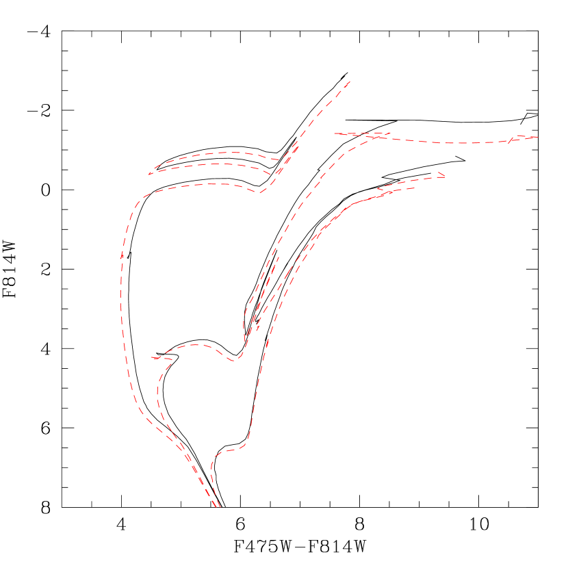
Figure 5: A set of $Z=0.008$ isochrones from Marigo et al. (2008) in the ACS/WFC system, extincted by $A_{V}=6$ mag according to two different prescriptions: adopting the star-to-star interstellar extinction coefficients as described in this paper (continuous lines) and adopting the coefficients derived from a yellow dwarf at the regime of low interstellar extinction (dashed lines). The isochrone ages are, from top-left to bottom-right, 0.1, 1, and 10 Gyr.

Figure 5 presents a practical application of the star-to-star interstellar extinction coefficients derived in this work, as compared to the usual approximation of applying a single set of coefficients for all stars and independently of the actual amount of total extinction. In the figure, one can notice that a set of isochrones extincted by $A_{V}=6$ mag in the correct (star-to-star) way, is narrower in colour (by about 0.3 mag in F475W–F84W) than an isochrone extincted by the same $A_{V}$ but using a single set of coefficients derived from a low-extinction yellow dwarf. Moreover, using the right interstellar extinction coefficients produces brighter red giants than in the case of constant coefficients. This latter effect is striking in the comparison between the AGB sequences at the top-right corner of Fig. 5.

Although the $A_{V}=6$ mag case is rather extreme, it well illustrates the effect of star-to-star interstellar extinction. Whether this effect is important depends on the photometric accuracy of the data and models available, and on the passbands being considered. A very approximate rule is that, if one aims at reproducing data with an accuracy better than 0.05 mag in optical bands, star-to-star interstellar extinction should start being considered already at $A_{V}>2$ mag. A more consistent and safer rule, however, is to always take star-to-star extinction into consideration.

4 Application to isochrones and data release

Extensive tables with BC and interstellar extinction coefficients have been computed and are provided in the static web repository http://stev.oapd.inaf.it/dustyAGB07. The BC tables contain entries for all stars in our spectral library. The extinction coefficients instead have been computed for solar metallicity only. In fact, the effective temperature, and to a lower extent $\log g$, is the main parameter driving the changes in $A_{S_{\lambda}}/A_{V}$. We have verified that $A_{S_{\lambda}}/A_{V}$ values change very little as a function of [M/H]: as an example, for a dwarf star of $\mbox{$T_{\rm eff}$}=4000$ K extincted by $A_{V}=1$, $A_{\rm F475W}/A_{V}$ values differ by just 0.17 % between the $\mbox{\rm[{\rm M}/{\rm H}]}=0$ and $\mbox{\rm[{\rm M}/{\rm H}]}=-2.5$ cases.

Moreover, the interactive web interface http://stev.oapd.inaf.it/cmd allows the present tables to be applied to the theoretical isochrones from Padova that are based on Girardi et al. (2000) tracks. Taking into account the Bertelli et al. (1994) isochrone models for initial masses higher than 7 $M_{\odot}$, interpolated isochrones can be constructed for any age between 0 and 17 Gyr, and for any metallicity value between $Z=0.0001$ and $Z=0.03$ (see Girardi et al. 2002). A recent paper by Marigo et al. (2008) presents a substantial revision of these isochrones, with the replacement of the old TP-AGB tracks by much more detailed ones (cf. Marigo & Girardi 2007). The same isochrones will soon be extended to the planetary nebulae and white dwarfs stages.

A novelty in this latter web interface is the possibility of producing isochrones already incorporating the effect of interstellar extinction and reddening. This is done via interpolations in the tables of $BC_{S_{\lambda}}(A_{V})$, using $\log\mbox{$T_{\rm eff}$}$, $\log g$, and $A_{V}$ as the independent parameters. The dependence in metallicity is ignored since it is really minimal (with $\lesssim 0.2$ % differences in $A_{S_{\lambda}}/A_{V}$, going from the solar-metallicity to the very-metal poor cases). Therefore, the $BC_{S_{\lambda}}(A_{V})$ tables are prepared for $\mbox{\rm[{\rm M}/{\rm H}]}=0$ only, and the $BC_{S_{\lambda}}(A_{V})-BC_{S_{\lambda}}(0)$ corrections derived from these tables are applied at all metallicities. This conceptually simple procedure is completely equivalent to alternative ones based on the interpolation of $A_{S_{\lambda}}/A_{V}$ tables.

In this way, users of the web interface just need to specify the total interstellar extinction $A_{V}$, to apply the proper $A_{S_{\lambda}}$ value at every point in the isochrone in each filter passband. We remind that the traditional approach is to apply a single value of extinction $A_{S_{\lambda_{1}}}$ and reddening $A_{S_{\lambda_{1}}}-A_{S_{\lambda_{2}}}$ to all points along an isochrone – $A_{S_{\lambda_{1}}}$ and $A_{S_{\lambda_{2}}}$ being related to the total $A_{V}$ via constant multiplicative factors – then occasionally seeking for the $A_{V}$ value that best fits a certain kind of observations. Instead, by applying the proper $A_{S_{\lambda}}$ value to each isochrone point, we take into account its dependence on $T_{\rm eff}$, on $\log g$, and on the total $A_{V}$ itself. Our procedure will lead to both (1) the traditional overall translation of isochrones in the CMD, and (2) moderate changes in the isochrone shapes as interstellar extinction increases, especially for colours involving blue passbands and in the regime of high extinction. The changes in the isochrone shapes will not be noticeable for low extinctions (for $A_{V}\lesssim 2$ mag, in optical passbands) and/or for near-infrared passbands.

Moreover, the present tables of bolometric corrections, for the no-extinction case only, are being applied to Bertelli et al. (2008) isochrones, which cover a wide region of the helium–metal content $(Y,Z)$ plane.

5 A few comparisons with data

The present bolometric corrections and interstellar extinction coefficients for ACS and WFPC2 are part of a large database of transformations to many photometric systems (see Marigo et al. 2008 for the most updated version). Regarding the BC and colour-$T_{\rm eff}$ relations for non-C stars, they have just slightly changed – a few hundredths of magnitude at most – with respect to those presented by Girardi et al. (2002). Therefore the transformations presented in this paper are in fact already largely tested in the literature, in many papers that compared data and models seeking accuracies to within $\sim 0.05$ mag in colours. Most of these previous comparisons were however done in Johnson-Cousins, 2MASS and SDSS systems.

In the present paper we limit ourselves to a couple of simple comparisons between present models and observations in the ACS/WFC F475W, F606W and F814W pass-bands. These filters, together with F555W, are those in which most observations of resolved galaxies are available. These are also the filters used by the ANGST project.

The two panels of Fig. 6 compare $Z=0.0001$ and $Z=0.0004$ isochrones superimposed to the CMD of the globular cluster M92 in three band combinations: $(V-I)$, (F475W–F814W) and (F606W–F814W). The $VI$ data are from the Rosenberg et al. (2000) database, and has kindly been provided by A. Rosenberg. The F475W, F814W CMD has been obtained using archival data from the ACS LCID project and the F606W, F814W CMD using ACS archival data of P.ID. 9453 (see Brown et al. 2005). The isochrones have log(age/yr)=10.10 and 10.15, and are plotted from the lower main sequence up to the TRGB; additionally, we plot the zero-age horizontal branch from Girardi et al. (2000) tracks as derived by Palmieri et al. (2002). In all cases we have assumed a distance modulus $(m-M)_{0}=14.62$ (del Principe et al. 2005), and interstellar extinction $A_{V}=0.068$ following the Schlegel et al. (1998) maps. The cluster measured metallicity is $\mbox{\rm[{\rm Fe}/{\rm H}]}=-2.24$ (Zinn & West 1984); or $-2.16$ (Carretta & Gratton 1997), which would correspond to $Z=0.0001$ of Girardi et al. (2000) scaled-solar isochrones. This case is plotted in the upper panel. Note however that the $Z=0.0004$ isochrones (lower panel) seem to fit the cluster sequences best, especially the RGB slope and the position of the main sequence turn-off. Note that the different mismatches that can be appreciated go in the same direction in the ground-based and the ACS fit. These mismatches are likely to be associated to the theoretical isochrones themselves, rather than to the color transformations.

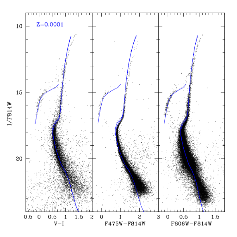
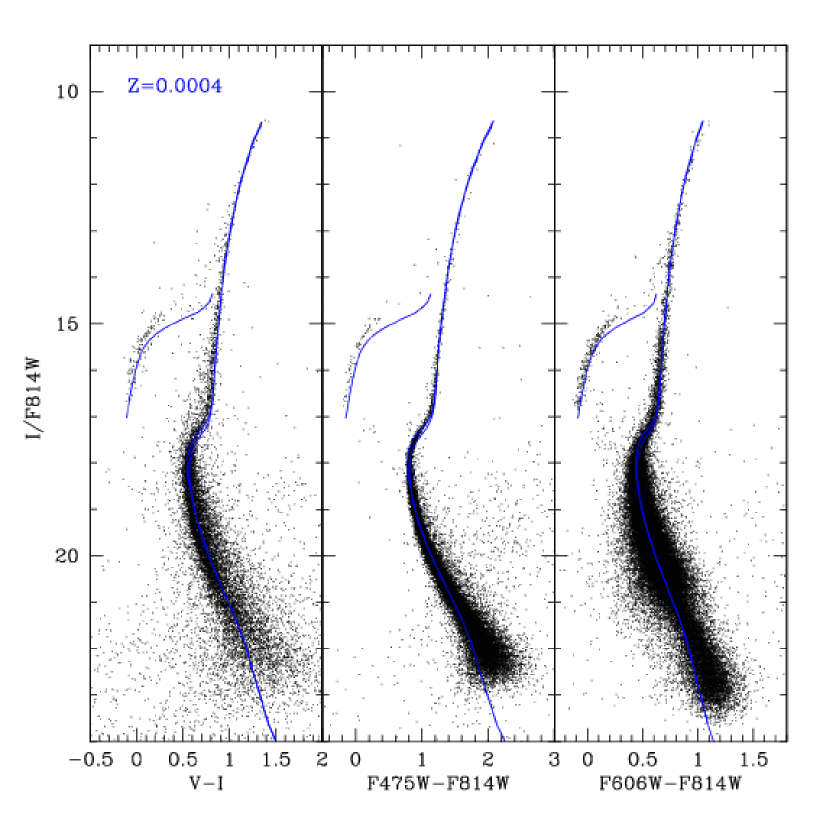
Figure 6: CMD of M92 in three different band combinations, compared with isochrones of metallicity $Z=0.0001$ and $0.0004$ as indicated in the labels. The isochrone ages are log(age/yr)=10.10 and 10.15. See the text for details.

This comparison with a nearby globular cluster illustrates the usefulness of the isochrones in the interpretation of star clusters in general, in which the photometry goes from the red giants down to the unevolved section of the main sequence. Most of the HST archival data refers instead to the composite stellar populations of nearby galaxies. Fig. 7 shows the case of field WIDE1 located about 13 arcmin along the major axis of the spiral galaxy NGC 253, observed with ACS/WFC for the ANGST project. Surprisingly, this region shows no sign of young stellar populations. A set of 10-Gyr old isochrones overimposed on the data CMDs would indicate a range of [M/H] going from about $-2$ to $0$. The observed CMD presents a striking decrease of stellar density above a certain level of the red giants, which obviously corresponds to the TRGB position. In Fig. 7, the green line marks the TRGB for a series of 10-Gyr-old isochrones of varying [Fe/H], displaced by a distance modulus of $27.6$ mag. It can be noticed that this line describes remarkably well the shape of observed boundary between the stellar-rich RGB and the less populated AGB. Although the precise position of this TRGB line is determined also by the quality of the underlying stellar models, its reproduction over a wide range in colour (covering more than $2$ mag in F475W–F814W, and more than $1$ mag in F606W–F814W) is clearly suggesting a correct behaviour of the set of BCs that has been applied.

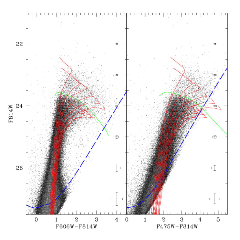
Figure 7: CMDs for the ACS Wide 1 pointing over NGC 253 (black and gray dots). The dashed line signals the 50 % completness limit of the ACS observations. The red lines are Marigo et al. (2008) 10-Gyr isochrones of metallicities $\mbox{\rm[{\rm M}/{\rm H}]}=(-2.0,-1.5,-1.0,-0.5,0.0)$, shifted by a distance modulus of 27.6. The green line marks the predicted locus of the TRGB for a more complete sequence of 10-Gyr isochrones with [M/H] increasing from $-2.3$ to $+0.1$.

6 Concluding remarks

In this paper we present tables of bolometric corrections and interstellar extinction coefficients, as a function of $T_{\rm eff}$, $\log g$, and [M/H], for the WFPC2 and ACS systems. We keep the original definition of the Vega magnitudes by Holtzman et al. (1995) and Sirianni et al. (2005), while adopting the latest accurate measurements of the Vega fluxes by Bohlin (2007). The tables are applied to theoretical isochrones in http://stev.oapd.inaf.it/cmd and http://stev.oapd.inaf.it/dustyAGB, where similar data for many other photometric systems can be found. A major novelty of this work is that interstellar extinction coefficients are computed and applyed star-by-star, so that isochrones present not only the overall shift in the CMDs as extinction increases, but also the subtle changes in their shape. We have made simple comparisons of these isochrones with real data, but a more careful testing of the transformations is left to future papers, and to the interested readers.

To the users of these HST isochrones, suffice it to recall a few general caveats, which apply to all photometric systems: First, our results are based on theoretical model atmospheres and spectral energy distributions, which are known not to be accurate at the hundredths-of-magnitude level, especially for the coolest stars. The same applies to Bohlin’s (2007) Vega spectrum, which has uncertainties of 1–2 % in the optical. Moreover, the results for narrow-band filters are particularly sensitive to errors in line opacity lists, and hence may be more uncertain. Overall, we expect the BCs for broad-band filters to be accurate to within $\sim 0.05$, with errors in colours being somewhat smaller. If we consider all the other uncertainties involved in the analysis of HST photometric data – including for instance the substantial uncertainties in the metallicity distribution and interstellar extinction curves of nearby galaxies – errors of this magnitude may be considered as acceptable.

The data provided in this paper are not conceived as a static set of tables, but rather as a database that will be revised and/or extended as soon as there is a significant improvement on the input ingredients – comprising the spectral flux libraries, the reference Vega spectrum, filter transmission curves, the interstellar extinction curve, and the isochrone sets to which the transformations are applied. An important extension is the inclusion of tables for the WFC3 camera (Bond et al. 2006), which will soon replace WFPC2 after HST Servicing Mission 4. Preliminary tables for WFC3 are already provided in the present database since they may be useful in the preparation for HST Cycle 17. They were derived in the same way as WFPC2 and ACS tables, using filter throughputs from SYNPHOT/STSDAS v3.7 files available at January 15, 2008. The WFC3 data will be replaced as soon as revised throughputs are released by the WFC3 team.

References

- Allard et al. (2000) Allard, F., Hauschildt, P. H., Alexander, D. R., Ferguson, J. W., & Tamanai, A. 2000a, in From Giant Planets to Cool Stars, ASP Conference Series, Vol. 212. Eds. Caitlin A. Griffith & Mark S. Marley (San Francisco: ASP), p. 127
- Allard et al. (2000) Allard, F., Hauschildt, P. H., & Schwenke, D. 2000b, ApJ, 540, 1005
- Allard et al. (2001) Allard, F., Hauschildt, P. H., Alexander, D. R., Tamanai, A., & Schweitzer, A. 2001, ApJ, 556, 357
- Bahcall et al. (1995) Bahcall, J. N., Pinsonneault, M. H., & Wasserburg, G. J. 1995, Reviews of Modern Physics, 67, 781
- Bedin et al. (2005) Bedin, L. R., Cassisi, S., Castelli, F., Piotto, G., Anderson, J., Salaris, M., Momany, Y., & Pietrinferni, A. 2005, MNRAS, 357, 1038
- Bertelli et al. (1994) Bertelli, G., Bressan, A., Chiosi, C., Fagotto, F., & Nasi, E. 1994, A&AS, 106, 275
- Bertelli et al. (2008) Bertelli, G., Girardi, L., Marigo, P., & Nasi, E. 2008, A&A, in press, ArXiv e-prints, 803, arXiv:0803.1460
- (8) Bessell, M.S., 1990, PASP, 102, 1181
- Bessell et al. (1998) Bessell, M. S., Castelli, F., & Plez, B. 1998, A&A, 333, 231
- Bohlin (2007) Bohlin, R. C. 2007, in The Future of Photometric, Spectrophotometric and Polarimetric Standardization, ASP Conference Series, Vol. 364, ed. C. Sterken, San Francisco: Astronomical Society of the Pacific, p. 315
- (11) Bond, H.E., et al. 2006, “Wide Field Camera 3 instrument mini-Handbook, Version 3.0” (Baltimore: STScI)
- (12) Brown, T.M., Ferguson, H.C., Smith, E., Guhathakurta, P., Kimble, R. A., Sweigart, A.V., Renzini, A., Rich, R.M., VandenBerg, D.A. 2005, AJ, 130, 1693
- (13) Cardelli, J.A., Clayton, G.C., Mathis, J.S. 1989, ApJ, 345, 245
- Castelli et al. (1997) Castelli, F., Gratton, R. G., & Kurucz, R. L. 1997, A&A, 318, 841
- (15) Castelli, F., & Kurucz, R. L., 2003, in Modelling of Stellar Atmospheres, proceedings of IAU Symposium 210, eds. N. Piskunov, W.W. Weiss, & D.F. Gray, Astronomical Society of the Pacific, p. A20
- (16) Carretta, E. & Gratton, R.G. 1997, A&ASS,121, 95
- (17) Chabrier G., Baraffe I., Allard F., Hauschildt P.H., 2000, ApJ, 542, 464
- Chiosi et al. (1997) Chiosi, C., Vallenari, A., & Bressan, A. 1997, A&AS, 121, 301
- Cioni et al. (2006) Cioni, M.-R. L., Girardi, L., Marigo, P., & Habing, H. J. 2006, A&A, 448, 77
- (20) Del Principe, M., Piersimoni, A., Bono, G., Di Paola, A., Dolci, M. & Marconi, M. 2005, AJ, 129, 2714
- Dotter et al. (2007) Dotter, A., Chaboyer, B., Jevremović, D., Baron, E., Ferguson, J. W., Sarajedini, A., & Anderson, J. 2007, AJ, 134, 376
- (22) Finley, D.S., Koester, D., Basri, G. 1997, ApJ, 488, 375
- Fluks et al. (1994) Fluks, M. A., Plez, B., The, P. S., de Winter, D., Westerlund, B. E., & Steenman, H. C. 1994, A&AS, 105, 311
- (24) Forbes, J.D. 1842, Phil. Trans., 132, 225
- Girardi et al. (2000) Girardi, L., Bressan, A., Bertelli, G., & Chiosi, C. 2000, A&AS, 141, 371
- Girardi et al. (2002) Girardi, L., Bertelli, G., Bressan, A., Chiosi, C., Groenewegen, M. A. T., Marigo, P., Salasnich, B., & Weiss, A. 2002, A&A, 391, 195
- Girardi et al. (2005) Girardi, L., Groenewegen, M. A. T., Hatziminaoglou, E., & da Costa, L. 2005, A&A, 436, 895
- (28) Grebel, E.K., & Roberts, W.J. 1995, A&AS, 109, 293
- Holtzman et al. (1995) Holtzman, J. A., Burrows, C. J., Casertano, S., Hester, J. J., Trauger, J. T., Watson, A. M., & Worthey, G. 1995, PASP, 107, 1065
- (30) Homeier, D., Koester, D., Hagen, H.-J., et al. 1998, A&A, 338, 563
- Lejeune (2002) Lejeune, T. 2002, in Observed HR Diagrams and Stellar Evolution, ASP Conference Proceedings, Vol. 274, eds. Thibault Lejeune & João Fernandes, San Francisco: Astronomical Society of the Pacific, p.159
- O’Donnell (1994) O’Donnell, J. E. 1994, ApJ, 422, 158
- (33) Loidl, R., Lançon, A., & Jørgensen, U.G. 2001, A&A 371, 1065
- Maíz Apellániz (2006) Maíz Apellániz, J. 2006, AJ, 131, 1184
- Marigo & Girardi (2001) Marigo, P., & Girardi, L. 2001, A&A, 377, 132
- Marigo & Girardi (2007) Marigo, P., & Girardi, L. 2007, A&A, 469, 239
- Marigo et al. (2003) Marigo, P., Girardi, L., & Chiosi, C. 2003, A&A, 403, 225
- Marigo et al. (2008) Marigo, P., Girardi, L., Bressan, A., Groenewegen, M. A. T., Silva, L., & Granato, G. L. 2008, A&A, in press, ArXiv e-prints, 711, arXiv:0711.4922
- Palmieri et al. (2002) Palmieri, R., Piotto, G., Saviane, I., Girardi, L., & Castellani, V. 2002, A&A, 392, 115
- Recio-Blanco et al. (2005) Recio-Blanco, A., et al. 2005, A&A, 432, 851
- (41) Rosenberg, A., Aparicio, A., Saviane, I. & Piotto, G. 2000, A&ASS, 145, 451
- Salasnich et al. (2000) Salasnich, B., Girardi, L., Weiss, A., & Chiosi, C. 2000, A&A, 361, 1023
- (43) Schlegel, D.J., Finkbeiner, D.P. & Davis, M. 1998, ApJ, 500, 525
- Sirianni et al. (2005) Sirianni, M., et al. 2005, PASP, 117, 1049
- (45) Vanhollebeke, E., Groenewegen, M.A.T., Girardi, L. 2008, A&A, submitted
- (46) Zinn, R. & West, M.J. 1984, ApJS, 55, 45