Multistable Solitons in Higher-Dimensional Cubic-Quintic Nonlinear Schrödinger Lattices

Abstract

We study the existence, stability, and mobility of fundamental discrete solitons in two- and three-dimensional nonlinear Schrödinger lattices with a combination of cubic self-focusing and quintic self-defocusing onsite nonlinearities. Several species of stationary solutions are constructed, and bifurcations linking their families are investigated using parameter continuation starting from the anti-continuum limit, and also with the help of a variational approximation. In particular, a species of hybrid solitons, intermediate between the site- and bond-centered types of the localized states (with no counterpart in the 1D model), is analyzed in 2D and 3D lattices. We also discuss the mobility of multi-dimensional discrete solitons that can be set in motion by lending them kinetic energy exceeding the appropriately crafted Peierls-Nabarro barrier; however, they eventually come to a halt, due to radiation loss.

1 Introduction

A large number of models relevant to various fields of physics is based on discrete nonlinear Schrödinger (DNLS) equations [1]. A realization of the one-dimensional (1D) DNLS model in arrays of parallel optical waveguides was predicted in Ref. [2], and later demonstrated experimentally, using an array mounted on a common substrate [3]. Multi-channel waveguiding systems can also be created as photonic lattices in bulk photorefractive crystals [4]. Discrete solitons are fundamental self-supporting modes in the DNLS system [1]. The mobility [5, 6] and collisions [6, 7] of discrete solitons have been studied in 1D systems of the DNLS type with the simplest self-focusing cubic (Kerr) nonlinearity. The DNLS equation with the cubic onsite nonlinearity is also a relevant model for the Bose-Einstein condensate (BEC) trapped in deep optical lattices [8].

A more general discrete cubic nonlinearity appears in the Salerno model [9], which combines the onsite cubic terms and nonlinear coupling between adjacent sites. A modification of the Salerno model, with opposite signs in front of the onsite and inter-site cubic terms, makes it possible to study the competition between self-focusing and defocusing discrete nonlinearities. This has been done in both 1D [10] and 2D [11] settings.

Lattice models with saturable onsite nonlinear terms have been studied too. The first model of that type was introduced by Vinetskii and Kukhtarev in 1975 [12]. Bright solitons in this model were predicted in 1D [13] and 2D [14] geometries. Lattice solitons supported by saturable self-defocusing nonlinearity were created in an experiment conducted in an array of optical waveguides built in a photovoltaic medium [15]. Dark discrete solitons were also considered experimentally [16] and theoretically [17] in the latter model.

The experimental observation of optical nonlinearities that may be fitted by a combination of self-focusing cubic and self-defocusing quintic terms [18] suggests to study the dynamics of solitons in the NLS equation with cubic-quintic (CQ) nonlinearity. A family of stable exact soliton solutions to the 1D continuum NLS equation of this type is well known [19]. The possibility to build an array of parallel waveguides using optical materials with the CQ nonlinearity lends relevance to the consideration of the DNLS equation with the onsite nonlinearity of the CQ type. In particular, this DNLS equation arises as a limit case of the continuum CQ-NLS equation which includes a periodic potential in the form of periodic array of rectangular channels, i.e., the Kronig-Penney lattice. Families of stable bright solitons were found in 1D [20] and 2D [21] versions of the latter model (the latter one with a “checkerboard” 2D potential supports both fundamental and vortical solitons).

The findings of a CQ-DNLS model may also be relevant to the case of a self-attractive BECs confined in a 2D plane by a “pancake”-shaped trap combined with a sufficiently strong 2D optical-lattice potential (although quantum effects such as a superfluid to Mott insulator transition are also relevant in the latter [22]). The condensate trapped in each individual potential well of this configuration is described by the Gross-Pitaevskii equation with an extra self-attractive quintic term which accounts for the deviation of the well’s shape from one-dimensionality [23]. The tunneling of atoms between adjacent potential wells in this setting is approximated by the linear coupling between sites of the respective lattice.

The simplest stationary bright solitons, of the unstaggered type (without spatial oscillations in the solitons’ tails), have been studied in the 1D version of the CQ-DNLS model in Ref. [24]. It was demonstrated that this class of solitons includes infinitely many families with distinct symmetries. The stability of the basic families was analyzed, and bifurcations between them were explored in a numerical form, and by means of a variational approximation (VA). Dark solitons in the same model were recently studied [25] and, in another very recent work, staggered 1D bright solitons as well as the mobility of unstaggered ones have been investigated [26].

The aim of the present work is to study the existence, stability, and mobility of bright discrete solitons in two- and three-dimensional (2D and 3D) NLS lattices with the nonlinearity of the CQ type. As suggested by the previous works, especially Ref. [24], the competition of the self-focusing cubic and self-defocusing quintic nonlinearities in the setting of the discrete model may readily give rise to multi-stability of discrete solitons, which is not possible in the ordinary cubic DNLS model [27], nor in the discrete CQ model where both nonlinear terms are self-focusing [28]. In addition to that, one may expect that the CQ model shares many features with those including saturable nonlinearity [29, 14], such as enhanced mobility of multidimensional discrete solitons (as mentioned above, mobile discrete solitons can be readily found in the 1D CQ-DNLS equation [26]).

The paper is organized as follows: in the next section, we introduce the model and outline the method used to construct the multi-dimensional discrete solitons. In Sec. 3, we focus on stability and existence regions for 2D discrete solitons, and the respective bifurcations. Mobility of the 2D solitons on the lattice is studied in Sec. 4. Section 5 reports extensions of these results to 3D latices. In Sec. 6 we report analytical results obtained by means of a VA, and Sec. 7 concludes the paper.

2 The model

In dimensionless form, the 2D DNLS equation with the onsite nonlinearity of the CQ type has the following form:

$$i\dot{\psi}_{n,m}+C\Delta^{(2)}\psi_{n,m}+2|\psi_{n,m}|^{2}\psi_{n,m}-|\psi_{n,m}|^{4}\psi_{n,m}=0,$$ (1)

where $\psi_{n,m}$ is the complex field at site {$n,m$} (the amplitude of the electromagnetic field in an optical fiber, or local mean-field wave function in BEC), $\dot{\psi}\equiv d\psi/dt$, and $C>0$ is the coupling constant of the lattice model. We assume an isotropic medium, hence the discrete Laplacian is taken as

$$\Delta^{(2)}\psi_{n,m}\equiv\psi_{n+1,m}+\psi_{n-1,m}+\psi_{n,m+1}+\psi_{n,m-1}-4\psi_{n,m}.$$ (2)

The CQ nonlinearity is represented by the last two terms in Eq. (1).

Equation (1) conserves two dynamical invariants: norm (or power, in terms of optics),

$$M=\sum_{n,m}\left|\psi_{n,m}\right|^{2},$$ (3)

and energy (Hamiltonian),

$$H = \sum_{n,m}\left[C(|\psi_{n+1,m}-\psi_{n,m}|^{2}+|\psi_{n,m+1}-\psi_{n,m}|^{2})\right.$$ (4)

$$\phantom{\sum_{n,m}}\left.-|\psi_{n,m}|^{4}+\frac{1}{3}|\psi_{n,m}|^{6}\right].$$

The conserved quantities play an important role in the analysis of the mobility of discrete solitons, see Sec. 4 below.

Steady state solutions are sought for in the usual form, $\psi_{n,m}=u_{n,m}\exp(-i\mu t)$, where $\ \mu$ is the real frequency, and the real stationary lattice field $u_{n,m}$ satisfies the following discrete equation:

$$\mu u_{n,m}+C\Delta^{(2)}u_{n,m}+2u_{n,m}^{3}-u_{n,m}^{5}=0.$$ (5)

More general solutions carrying topological charge, for which stationary field $u_{n,m}$ is complex, fall outside of the scope of the present work, and will be considered elsewhere.

In one dimension, bright-soliton solutions of Eq. (5) can be found as homoclinic orbits of the corresponding two-dimensional discrete map [30]. This technique was used to construct 1D soliton solutions to the CQ-DNLS model in Ref. [24]. Since this method is not available in higher dimensions, we construct the solutions starting from the anti-continuum limit, $C\rightarrow 0$, and perform parameter continuation to $C>0$. A multidimensional version of the VA can also be used to construct solutions for small values of $C$, see Sec. 6 below.

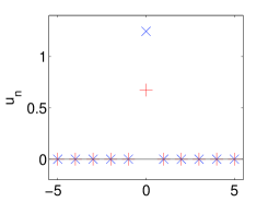
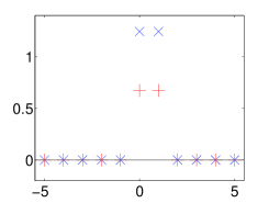
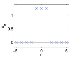
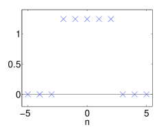
Figure 1: (Color online) Solutions to Eq. (1) for $(\mu,C)=(-0.7,0)$, which are used as seeds to find nontrivial solutions at $C>0$ (only a 1D slice is shown, see Fig. 3 for profiles in two dimensions). Top left: “Tall” (blue cross markers) and “short” (red plus markers) site-centered solutions. Top right: “Tall” and “short” bond-centered solutions. Bottom: wider extensions of the “tall” site-centered solution.

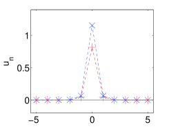
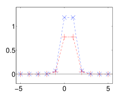
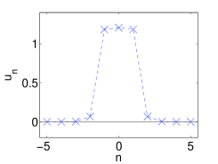
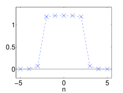
Figure 2: (Color online) The continuation to $C=0.1$ of the solutions shown in Fig. 1.

In Ref. [24], two fundamental types of solutions were studied: site-centered and bond-centered solitons. Each family of solutions was further subdivided into two sub-families, which represent “tall” and “short” solutions for given parameter values. Moreover, each sub-family contains, depending on the value of $C$, wider solutions that may be built by appending extra excited sites to the soliton. The reason for the co-existence of the tall and short sub-families is clearly seen in the anti-continuum. If $C=0$, Eq. (5) reduces to the following algebraic equation:

$$\mu u_{n,m}+2u_{n,m}^{3}-u_{n,m}^{5}=0,$$ (6)

which has at most five real solutions, viz.,  four nontrivial ones,

$$u_{n,m}=\displaystyle\pm\sqrt{1\pm\sqrt{1+\mu}},$$ (7)

and $u_{n,m}=0$ (note that these are also fixed points of the above-mentioned discrete map in the 1D case). Obviously, Eq. (7) gives, at most, two different non-trivial amplitudes, that may be continued to $C>0$, giving rise to tall and short solitons respectively. To build wider solutions, one has to consider multiple sites with the nonzero field. Using the $C=0$ solutions as seeds, we are able to generate a large family of solutions in the $(\mu,C)$ parameter plane, as shown in Figs. 1 and 2. It is found that all the wide solutions tend to disappear through saddle-node collisions between the tall and short solutions as $C$ increases, similarly to what is the case for the cubic DNLS problem, as discussed in Ref. [31].

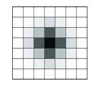
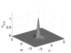
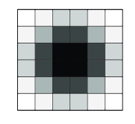
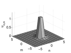
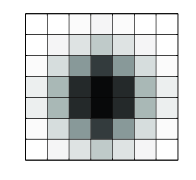
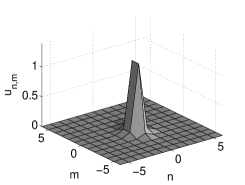
Figure 3: Left (from top to bottom): Contour plots of solutions of the site-centered, bond-centered, and hybrid types for $(\mu,C)=(-0.7,0.1)$. Right: The corresponding 3D plots.

Another fundamental type of solution that arises in higher-dimensional lattices is a hybrid between the site-centered and the bond-centered solutions along the two spatial directions, see bottom panels in Fig. 3. This type of hybrid solution was considered previously in the case of the cubic DNLS model in Ref. [32]. We only consider these three symmetric types of localized states, namely the bond-centered, site-centered, and hybrid ones (see Fig. 3), together with their intermediate asymmetric counterparts (see Fig. 8(c) for an example). The hybrid solution admits other natural variations, namely any combination of the various types of bond-centered solutions along one axis and any site-centered profile along the other. Since their behaviors are very similar, we consider only one such type of solutions.

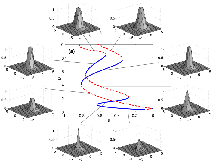
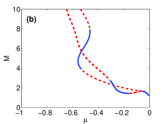
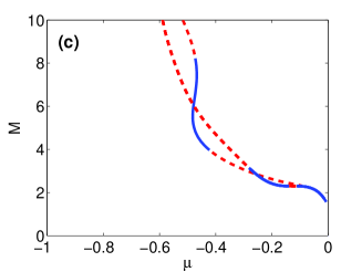
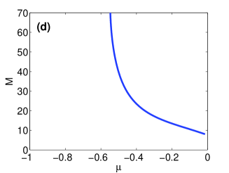
Figure 4: (Color online) (a) Power ($M$) versus $\mu$ for $C=0.1$, and respective profiles. Bottom (from left to right): Power diagrams, for (b) $C=0.3$, (c) $C=0.4$, and (d) $C=2.0$, of the bond-centered and site-centered solutions. For low values of $C$ the co-existence of multiple solutions at different values of $\mu$ is obvious. The “snaking” pattern gets stretched as $C$ increases, slowly diminishing the number of solutions until a single solution is left. Stable and unstable solutions are represented by solid (blue) and dashed (red) curves, respectively.

3 The existence and stability of stationary solutions

Detailed existence and stability regions of all above-mentioned solutions are quite intricate and particularly hard to detect. As described for the 1D case in Ref. [24] and mentioned above, we expect in the 2D case the existence of a large family of solutions at low values of $C$, which gradually annihilate, through a series of bifurcations, as $C\rightarrow\infty$ (see Ref. [31] for a detailed description of the termination scenaria, typically through saddle-node or pitchfork bifurcations, for the various families of the basic discrete solitons as the coupling parameter is increased). By plotting the power $M$ for various types of the solutions (site-centered, bond-centered, and hybrid, each with various widths) at fixed values of $C$ against frequency $\mu$, it is possible to trace the trend followed by the solutions (see Fig. 4). For $C=0$, the exact power for each solution can be found. A snake like pattern extending from $\mu=-1$ to $\mu=0$ exists and continues for arbitrarily large powers. This “snaking” is also displayed for different values of $C>0$ in Fig. 4. Branches of the $M(\mu)$ curve with higher powers correspond to wider solutions. A typical progression observed as one follows the $M(\mu)$ curve from bottom (low power) to top (high power) is switching between short and tall solutions with gradually increasing width. For example, the first branch, which represents short narrow solutions, collides with a branch of tall narrow solutions, which then collides with a set of short wide solutions, and so on. As the coupling strength increases, the power curve gets stretched upward. Following the stretching, the solutions gradually vanish, until there remains a single profile. Similar to what was found in cubic DNLS equation in Ref. [33] the bright stationary solutions in the CQ model also bifurcate from plane waves (near $\mu\approx 0$ for the CQ model). It is worthwhile to highlight here the increased level of complexity of the relevant $M(\mu)$ curves in the cubic-quintic model (due to the interplay of short and tall solution branches) in comparison to its cubic counterpart of Ref. [32], which features a single change of monotonicity (and correspondingly of stability) between narrow and tall (stable) and wide and short (unstable) solutions.

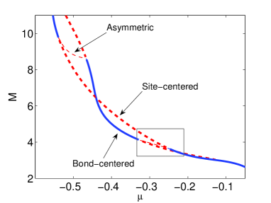
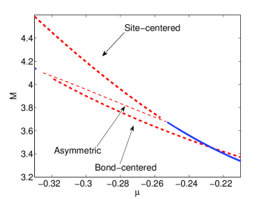
Figure 5: (Color online) Top: Pitchfork bifurcations of the bond-centered solutions and site-centered solutions for lattice coupling constant $C=0.5$. Hybrid solutions are omitted here for clarity. Bottom: Zoom of the bifurcation scenario depicted by the rectangular region in the top panel.

Reference [33] provides heuristic arguments for the existence of energy thresholds for a large class of discrete systems with dimension higher than some critical value. This claim was proved in Ref. [34] for DNLS models with the nonlinearities of the form $|\psi_{n}|^{2\sigma+1}\psi_{n}$ and for chains of NLS equations. As can be discerned in Fig. 4, such thresholds also exist in the case of the cubic-quintic nonlinearity.

In Ref. [24] a stability diagram for the discrete solitons in the 1D model was presented in the $(\mu,C)$ plane, which gave a clear overview of the situation. However, in the present situation, the $M(\mu)$ curves for various fixed values of $C$, such as those displayed in Fig. 4, provide for a better understanding of relationships between different solutions. For example, in the $(\mu,C)$ diagram, it would appear that the taller solutions cease to exist at $(\mu,C)\approx(-0.6,0.4)$. However, the respective $M(\mu)$ curve shows that narrow and wide solitons become indistinguishable at this point, and deciding which solution, short or tall, is annihilated becomes quite arbitrary.

A numerical linear stability analysis was performed in the usual way (see Ref. [24] for details) to investigate the stability of each of the solution branches. As one follows a $M(\mu)$ curve from bottom to top, the stability is typically swapped around each turning point, as seen in Fig. 4. However, the stability is not switched exactly at these points, as this happens via asymmetric solutions (see below).

Similar to the 1D model, a pitchfork-like bifurcation occurs between the site- and bond-centered discrete solitons. This is more clearly seen in Fig. 5. For $C=0.5$, the bond-centered solution loses its stability in a neighborhood of $\mu\approx-0.53$, and asymmetric solutions are created there. There are multiple asymmetric solutions in this case, but only one curve appears in Fig. 5, since each one is just a rotation of the other, hence they have the same power. The bond-centered solution loses its stability before the site-centered solution regains its stability; in fact, the site-centered soliton regains the stability exactly when the asymmetric solutions collide with it. This sort of stability exchange occurs throughout the $M(\mu)$ curve. The top panel of Fig. 5 shows two such bifurcations, with a zoom of one of them shown in the bottom panel.

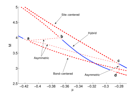
Figure 6: (Color online) Bifurcations for $C=0.4$ showing that all three fundamental modes (site-centered, bond-centered, and hybrid) are all connected to each other via stability exchange with asymmetric solutions. Two asymmetric solutions are created where the bond-centered solution loses stability at the bifurcation point labeled by ‘a’ in the diagram. One of these asymmetric solutions is connected to the hybrid solution at ‘b’ and the other is connected to the site-centered solution at point ‘c’. A third type of asymmetric solution also emanates from the bifurcation point ‘c’ which is connected to the hybrid solution at ‘d’.

Figure 6 shows again a site-centered solution connected to a bond-centered solution but also features a connection of the site- and bond-centered solutions via the hybrid solution. So not only are all variations (tall, short, narrow, etc) within each mode connected, as shown by the snake like power curves, but all the fundamental modes (bond-centered, site-centered, hybrid) are also connected.

We stress that the stability regions of the above mentioned fundamental modes are disjoint in regions where they each have roughly the same power and, unlike the 1D model, the asymmetric solutions are unstable. These features can be seen in Figs. 5 and 6. Note that the multi-stability of symmetric solutions still occurs in this case due to the existence of arbitrarily wide solutions at fixed values of $C$ (see Fig. 4). As a general comment, it should be noted that many of the features of the 2D cubic-quintic model (such as e.g., the existence of unstable asymmetric solutions, and their connecting the fundamental modes) can also be observed in the case of the saturable model [14], although in the present case of the cubic-quintic model, the relevant phenomenology is even richer due to, for instance, the existence of multiple (i.e., tall and short) steady states.

4 The mobility

In one dimension, traveling solutions can be found in the form

$$\psi_{n}=u(n-vt)e^{i\mu t},$$ (8)

where $v$ is a real velocity. Substitution of this expression in the 1D DNLS model yields the following advance-delay differential equation

$$0 = -i[v\dot{u}(z)+i\mu u(z)]+2|u(z)|^{2}u(z)-|u(z)|^{4}u(z)$$ (9)

$$+C\left[u(z+1)+u(z-1)-2u(z)\right],$$

where $z=n-vt$. Stationary solutions are said to be translationally invariant if the function $u_{n}=u(nh)$, where $h$ is the lattice spacing, can be extended to a one-parameter family of continuous solutions, $u(z-s)$, of the advance-delay equation (9) with $v=0$. Solutions of this type have been found in other lattice models (see Ref. [35, 36] and references therein). Localized solutions with non-oscillatory tails in similar models for $v\neq 0$, have been found in Ref. [29, 37] by solving a respective counterpart of Eq. (9). If translationally invariant solutions exist, then the sundry modes (bond-centered, site-centered, etc.) are generated by the same continuous function $u(z-s)$, each with a corresponding value of $s$. The translationally invariant solutions occur (i) at transparency points, which are points in the parameter space where solutions exchange their stability, and (ii) if the Peierls-Nabarro (PN) barrier vanishes; the barrier being defined as the difference in energy between the site-centered and bond-centered solutions. Note that (i) and (ii) are necessary but not sufficient conditions for the existence of translationally invariant solutions. For higher-dimensional lattices, translationally invariant solutions for DNLS-like models have not been found yet. However, effectively mobile lattice solitons have been found in 2D models in regions of the parameter space where the PN barrier is low (enhanced mobility). This has been the case both for quadratic nonlinearities [38] and in the vicinity of stability exchanges for saturable models [14]. The resulting mobile solutions radiate energy and eventually come to a halt. Exact solutions of the corresponding advance-delay differential equation, if they exist, would experience no radiation losses and propagate indefinitely, which is why they are called radiationless solutions [29]. As mentioned above for translationally invariant solutions, radiationless solutions have also not been yet been found in higher-dimensional lattices. In fact, it is an important open question whether such solutions exist typically, since the single tail resonance appropriately made to vanish in Ref. [29] to obtain such exponentially localized traveling solutions in 1D settings, acquires infinite multiplicity in higher dimensional settings. Thus, the admittedly straightforward technique of identifying regions of enhanced mobility may be the only possible method in higher dimensional DNLS problems.

The goal is to “kick” the stationary solutions into motion. From a Hamiltonian point of view, the real part of the solution corresponds to position and the imaginary part to momentum [27]. Therefore, in order to set it into motion one should apply a perturbation that will alter the imaginary part of the solution in an asymmetric way, and thus providing it with the necessary momentum to move. To this end, we apply a “kick” of the form

$$u_{n,m}(0)=u_{n,m}e^{i(k_{n}n+k_{m}m)},$$ (10)

where $u_{n,m}$ is a stationary solution, and $k_{n}$, and $k_{m}$ are real wavenumbers. This method has been used in numerous studies in one-dimensional settings (cf. Refs. [27, 39]) and recently in two-dimensions [14]. Bright mobile solutions were studied in this way in the 1D CQ model in Ref. [28] and in greater detail (and for staggered solutions) in Ref. [26]. We present here results for a site-centered solution moving along a single axis only. Therefore we set $k_{n}\neq 0$ and $k_{m}=0$. Results for other solutions are similar. There are three qualitative scenarios that we have observed as result of the kick: (a) the kick is below some threshold value, $k_{n}<k_{\mathrm{depin}}$, and so the corresponding energy increase is too low to depin the solution, (b) the kick is greater than this threshold value, $k_{n}>k_{\mathrm{depin}}$, and the solution is set in motion eventually halting, or (c) the initial kick is so strong, $k_{n}>k_{\mathrm{disperse}}$, that the solution disperses. See Fig. 7 for examples of these three scenaria.

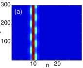
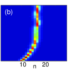
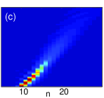
Figure 7: (Color online) Resulting density plots, of a one-dimensional slice along the axis of propagation, from imprinting momentum to a stationary soliton by means of the “kick” defined in Eq. 10. (a) $k<k_{\mathrm{depin}}$: the solution remains pinned at its initial position. (b) $k_{\mathrm{depin}}<k_{n}<k_{\mathrm{disperse}}$: the solution becomes mobile, but eventually comes to a halt due to radiation loss. (c) $k>k_{\mathrm{disperse}}$: the kick is so strong that the solution disperses.

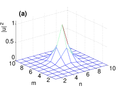
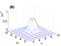
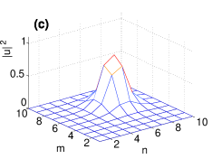
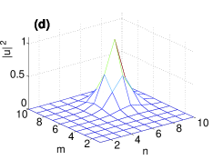
Figure 8: (Color online) Evolution of a site-centered soliton kicked along a diagonal. In the course of its motion, the traveling object takes on the (a) site-centered, (b) bond-centered, and (c) asymmetric profiles. This progression repeats starting again with the (d) site-centered profile until motion ceases due to radiation loss.

We are interested in areas of parameter space that provide good conditions for mobility for the kicked solutions. The PN barrier should provide some insight as to where these regions may be. While there is no standard formal definition of the PN barrier in higher dimensions, one may adopt a natural definition (as used in Ref. [14]), according to which the barrier is the largest energy difference, for a fixed norm of the soliton, between two stationary solutions of the system close to configurations that a discrete soliton must pass when moving adiabatically along the chosen lattice direction. This set of configurations includes asymmetric solutions, and, importantly in higher dimensions, the hybrid solutions too. For example, for a stationary site-centered soliton to become mobile along an axis, it must overcome barriers created by the asymmetric and hybrid states, since, in the course of its motion, its profile will change as follows: site-centered $\rightarrow$ asymmetric $\rightarrow$ hybrid $\rightarrow$ asymmetric $\rightarrow$ site-centered. If we chose to kick the soliton along the diagonal, then the same progression should be considered with the bond-centered state replacing the hybrid one (see Fig. 8). Here we use, for the definition of the PN barrier, fixed frequency $\mu$ rather than fixed norm $M$. We also consider the free energy $G=H-\mu M$ instead of the Hamiltonian as in Ref. [29] (note that Eq. (6) can be derived as $\partial G/\partial\psi_{n,m}^{*}=0$).

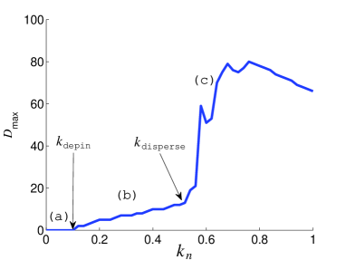
Figure 9: The maximum distance traveled as a function of the kicking strength $k_{n}$ for $(\mu,C)=(-0.225,0.4)$ and $t\in[0,800]$. The area labeled (a) in the graph represents values of $k_{n}$ that could not depin the solution (see Fig. 7.a). The area labeled by (b) consists of values of $k_{n}$ that yield a mobile solution (see Fig. 7.b) and in (c) the kick is so strong that the solution disperses (see Fig. 7.c). The threshold values, $k_{\mathrm{depin}}$ and $k_{\mathrm{disperse}}$ are also shown.

We kicked the site-centered solutions for various values of $k_{n}$, and estimated the corresponding threshold values. In Fig. 9 the maximum distance traveled,

$$D_{\mathrm{max}}(k)=\sup_{t\in[0,T_{0}]}\lfloor\langle n\rangle(t)\rfloor-\lfloor\langle n\rangle(0)\rfloor,\\$$ (11)

where the center of mass is computed by

$$\langle n\rangle(t)=\sum_{n,m}n|\psi_{n,m}(t)|^{2}/\sum_{n,m}|\psi_{n,m}(t)|^{2},$$ (12)

is plotted versus the kicking strength. The corresponding threshold values are also identified there.

It turns out that, the values of the thresholds are related to the PN barrier. The left panel in Fig. 10 shows the difference in free energy, $\Delta G_{\mathrm{hybrid}}=G_{\mathrm{site}}-G_{\mathrm{hybrid}}$ between the site-centered solution and the hybrid solution for fixed $C=0.4$ and $\mu\in[-0.3,-0.1]$. In each subpanel of the figure $D_{\mathrm{max}}$, as defined in Eq. (11), is plotted against the kicking strength for $t\in[0,800]$ for fixed $\mu$. In panel (i) the site-centered solution has more energy than the hybrid solution but is unstable and moves away from its initial position even for $k_{n}=0$. Panel (ii) represents parameter values where the site-centered solution has greater power and is stable. In this small “transparency window” of parameter space, there is also pair of unstable asymmetric solutions. In this region, we observed the best mobility (see Fig. 11). This is consistent with what was found in the saturable 2D DNLS [14] where good mobility was found where asymmetric solutions exist. In panel (iii) the threshold $k_{\mathrm{disperse}}$ is visible and the sign of $\Delta G_{\mathrm{hybrid}}$ has switched. In (iv) we see that the value of $k_{\mathrm{depin}}$ is increasing and $k_{\mathrm{disperse}}$ is decreasing as the PN barrier increases. Panel (v) corresponds to the maximum energy difference. This is also where the largest $k_{\mathrm{depin}}$ occurs. As the energy difference decreases once again as seen in (vi) the threshold $k_{\mathrm{disperse}}$ continues to decrease. This is also the case in panel (vii) as both thresholds approach $k_{n}=0$. Finally, for the unstable region in (viii) $k_{\mathrm{depin}}$ is once again zero.

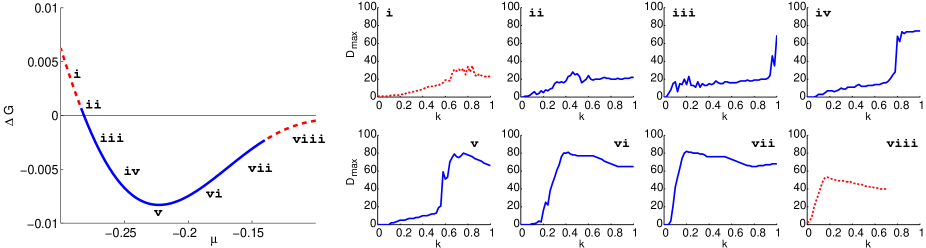
Figure 10: (Color online) Left: Plot of $\Delta G_{\mathrm{hybrid}}$ for various values of $\mu$ and fixed $C=0.4$. The remaining panels (i)–(viii) correspond to the maximum distance traveled versus kicking strength plots. See text for more details.

Figure 11: (Color online) Top: density plot for the site-centered soliton set in motion along the lattice axis for $(\mu,C)=(-0.282,0.4)$ and $k_{n}=0.5$. The choice of parameters fall in a “transparency window” where good mobility is observed, possibly due to the existence of a pair of asymmetric solutions. A one-dimensional slice along the axis of propagation (at $m=10$) is shown here. Bottom: zoom of the left panel of Fig. 10 near the “transparency window”. The difference of free energy of the site-centered solution and the pair of asymmetric solutions $\Delta G_{\mathrm{asymm}}=G_{\mathrm{site}}-G_{\mathrm{asymm}}$ is also shown. The energy added from the kick exceeds both of these differences.

We were unable to identify true transparency points in the present model (the 2D DNLS lattice with the CQ onsite nonlinearity), which seems to preclude the possibility of finding exact translationally invariant solutions. However, enhanced mobility was achieved by lending stationary solutions kinetic energy in cases where the PN barrier was low. These moving states gradually lose energy and get eventually trapped at some positions in the lattice. Solving higher-dimensional counterparts of Eq. (9) in the higher-dimensional lattice might reveal moving radiationless solutions, although, as we pointed out above, solutions to this (quite difficult) problem may not typically exist. It is worth mentioning in passing that the energy loss in the 1D discrete sine-Gordon lattice has been recently described using an averaged Lagrangian approach in Ref. [40].

5 Three-dimensional solutions

We will now briefly consider a 3D version of the CQ DNLS model. The respective counterpart of Eq. (5) is

$$i\dot{\psi}_{n,m,l} + C\Delta^{(3)}\psi_{n,m,l}+2|\psi_{n,m,l}|^{2}\psi_{n,m,l}$$ (13)

$$- |\psi_{n,m,l}|^{4}\psi_{n,m,l}=0,$$

where $\psi_{n,m,l}$ is the complex field at site {$n,m,l$}. In an isotropic medium, the discrete Laplacian is

$$\Delta^{(3)}\psi_{n,m,l} \equiv \psi_{n+1,m,l}+\psi_{n-1,m,l}+\psi_{n,m+1,l}+\psi_{n,m-1,l}$$ (14)

$$+\psi_{n,m,l+1}+\psi_{n,m,l-1}-6\psi_{n,m,l}.$$

We search for stationary solutions, $\psi_{n,m,l}=u_{n,m,l}\exp(-i\mu t)$, using the same method as in Sec. 2. The 2D soliton species have their natural 3D counterparts. As shown in Fig. 12, the extra dimension admits an additional type of a hybrid soliton.

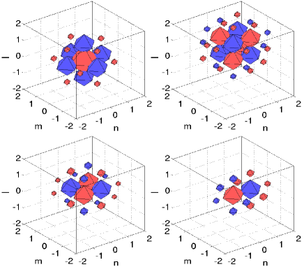
Figure 12: (Color online) Plot of the basic configurations in the 3D lattices using iso-contours. Top: plot of 3D site-centered (left) and bond-centered (right) solitons. Larger diamonds correspond to larger local amplitudes. Bottom: Two different types of 3D hybrid solutions. The different colors (arranged in a 3D check-board pattern) are solely used for clarity of presentation.

Figure 13 shows $M(\mu)$ curves for 3D bond-centered and site-centered solitons for $C=0.1$ and $C=0.7$. The figure illustrates that in the 3D case, similarly to the 2D case, the snake-like patterns are present for small values of coupling constant $C$ and are stretched as $C$ is increased. Similar results were obtained for the 3D hybrid solutions (results not shown here).

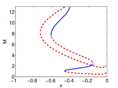
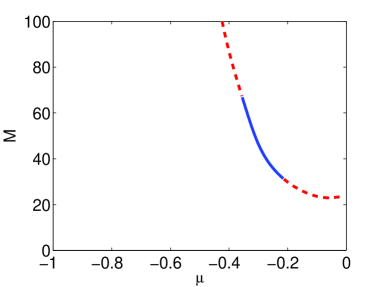
Figure 13: (Color online) The power of the site- and bond-centered solitons versus the frequency for $C=0.1$ (top) and $C=0.7$ (bottom) in the 3D lattice.

6 Variational approximation

Following the pattern of the VA developed in Ref. [24] for 1D discrete solitons in the CQ-DNLS model, it is possible to construct analytical approximations for the discrete solitons, and compare them to the numerical solutions described above. We present this approach for the 2D model, but the procedure is essentially the same in three dimensions. It is relevant to mention that the VA for 1D discrete solitons in models of the DNLS type was first developed in Ref. [41].

Solutions to the stationary version Eq. (1) are local extrema of the corresponding Lagrangian,

$${L} = \displaystyle\sum_{n,m=-\infty}^{\infty}\mu u_{n,m}^{2}+u_{n,m}^{4}-\frac{1}{3}u_{n,m}^{6}$$

$$- C\left[(u_{n+1,m}-u_{n,m})^{2}+(u_{n,m+1}-u_{n,m})^{2}\right]$$

[recall $\psi_{n,m}=u_{n,m}\exp(-i\mu t)$]. We approximate each soliton by a localized ansatz which makes it possible to evaluate the infinite sums in Eq. (6) in an explicit form. First, the following ansatz is used for the site-centered (sc) solution:

$$u_{m,n}^{\mathrm{(sc)}}=\left\{\begin{array}[]{ll}\beta&\mathrm{~{}if~{}}m=n=0,\\[4.30554pt] Ae^{-\alpha(|m|+|n|)}&\mathrm{~{}otherwise}\end{array}\right.$$ (16)

where $A,\beta,$ and $\alpha$ are real constants to be found from the Euler-Lagrange equations,

$$\frac{\partial L_{\text{eff}}}{\partial A}=\frac{\partial L_{\text{eff}}}{\partial\alpha}=\frac{\partial L_{\text{eff}}}{\partial\beta}=0,$$ (17)

$L_{\text{eff}}$ standing for Lagrangian (6) evaluated with ansatz (16). In particular, $\alpha$ is treated here as one of the variational parameters, in contrast to the 1D case, where it was expressed in terms of $\mu$ and $C$ by means of a relation obtained from the consideration of the linearized stationary equation for decaying “tails” of the soliton [24],

$$\alpha=\ln\left(\frac{a}{2}+\sqrt{\left(\frac{a}{2}\right)^{2}-1}\right),~{}a\equiv 2-\mu/C.$$ (18)

We have observed, based on numerous calculations, that treating $\alpha$ as a variational parameter yields the same relation for $\alpha$ in both the 2D and 3D models. This is consistent with solutions in the continuum model where it is known that the factor in the exponential tail is independent of the dimension.

Solutions predicted by the VA based on ansatz (16) provide for a good fit to the short and tall narrow solutions and the first subfamily of wide short solitons of the site-centered type, (see Fig. 14). At larger values of $C$, the VA-predicted solutions depart from the numerical ones, which is not surprising, as the exponential cusp implied by the ansatz is not featured by the discrete solitons in the strong-coupling (quasi-continuum) model.

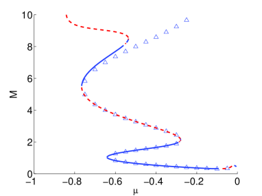
Figure 14: Numerical solutions (solid line) and the variational approximation (triangles) for the site-centered solitons at $C=0.1$ in the 2D lattice model. The approximation based on ansatz (16) is able to capture subfamilies of tall and short narrow solitons, and the branch of short wide solitons too.

Other solution types can be approximated by appropriately modified ansätze. In particular, the bond-centered (bc) soliton is based on a frame built of four points with equal amplitudes (see Fig. 3.b), whereas the hybrid (hy) soliton has just two points in its frame (see Fig. 3.c). Accordingly, the solitons of these types can be modeled by the following modifications of ansatz (16):

$$u_{m,n}^{\mathrm{(bc)}}=\left\{\begin{array}[]{ll}\beta&~{}m,n\in\{0,1\}\\[4.30554pt] Ae^{-\alpha(|m|+|n|)}&\mathrm{~{}if~{}}m,n<0\\[4.30554pt] Ae^{-\alpha(|m-1|+|n|)}&\mathrm{~{}if~{}}m>1,n<0\\[4.30554pt] Ae^{-\alpha(|m|+|n-1|)}&\mathrm{~{}if~{}}m<0,n>1\\[4.30554pt] Ae^{-\alpha(|m-1|+|n-1|)}&\mathrm{~{}otherwise}\end{array}\right.$$ (19)

and

$$u_{m,n}^{\mathrm{(hy)}}=\left\{\begin{array}[]{ll}\beta&~{}n=0,m\in\{0,1\}\\[2.15277pt] Ae^{-\alpha(|m|+|n|)}&\mathrm{~{}if~{}}m,|n|<0\\[2.15277pt] Ae^{-\alpha(|m-1|+|n|)}&\mathrm{~{}otherwise}\end{array}\right.$$ (20)

Further analysis demonstrates that the modified ansätze produce a good approximation for the short and tall narrow solutions at small $C$ but not any of the wide families (see Fig. 15).

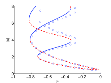
Figure 15: Numerical solutions (solid line) and the variational approximation for the bond-centered (squares) and hybrid (circles) solitons at $C=0.1$ in the 2D lattice model. The approximations based on the ansätze given in (19) and (20) respectively are able to capture subfamilies of tall and short narrow solitons.

We were also able to predict complicated bifurcations of the system by introducing the appropriately chosen asymmetric (asym) ansatz:

$$u_{m,n}^{\mathrm{(asym)}}=\left\{\begin{array}[]{ll}\beta_{1}&~{}n=0,m=0\\[2.15277pt] \beta_{2}&~{}n=0,m=1\\[2.15277pt] \beta_{3}&~{}n=1,m=0\\[2.15277pt] \beta_{4}&~{}n=1,m=1\\[2.15277pt] Ae^{-\alpha(|m-\zeta|+|n-\zeta|)}&\mathrm{~{}otherwise}\end{array}\right.$$ (21)

The intention here is to capture the bifurcations where the site-centered and bond-centered solutions are connected via an asymmetric solution. Therefore we have some idea a priori what the asymmetric solutions should look like and have chosen ansatz (21) accordingly. For $\zeta=0$ the ansatz has the form of a site-centered solution whereas for $\zeta=0.5$ it will represent a bond-centered solution. All intermediate values of $\zeta$ represent asymmetric solutions that are somewhere between a site-centered and bond-centered solution. Indeed, the computed value of $\zeta$ based on the variational approximation starts near $\zeta=0.5$ for parameter values where the asymmetric solution is almost connected to bond-centered solution, and slowly decreases to $\zeta=0$ as we alter the parameters until it collides with the site-centered solution (see Fig. 16).

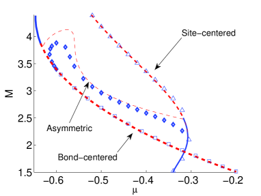
Figure 16: Bifurcations featuring the bond-centered, site-centered, and asymmetric solutions for $C=0.22$. Numerical solutions (lines) and its predicted counterparts using the VA based on the ansatz (21) (markers) are in good agreement. The asymmetric VA solution captures the main qualitative features of the $M(\mu)$ curve (e.g. the dramatic increase of power around $\mu\approx-0.55$) but slightly underestimates the power at the bifurcation points.

Finally we apply the methods to 3D lattice solitons using the following site-centered ansatz

$$u_{m,n,l}^{\mathrm{(sc)}}=\left\{\begin{array}[]{ll}\beta&\mathrm{~{}if~{}}m=n=l=0,\\[4.30554pt] Ae^{-\alpha(|m|+|n|+|l|)}&\mathrm{~{}otherwise}\end{array}\right.$$ (22)

where, for $C$ small enough, it also works well, see Fig. 17.

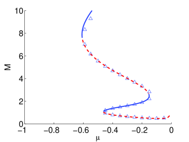
Figure 17: Numerical solution (solid line) and the variational approximation (triangles) for the site-centered solitons with $C=0.1$ using the ansatz given in (22) in the 3D DNLS lattice with cubic-quintic nonlinearities.

7 Conclusion

In this work, we have examined the existence, stability, and mobility of discrete solitons in 2D and 3D NLS lattices with competing (cubic-quintic, CQ) onsite nonlinearities. Some properties of the discrete solitons, such as existence of the solutions of tall and short types, each narrow and/or wide, resemble properties recently found in discrete solitons in the 1D counterpart of this model [24], as well as the 2D properties of models such as the one with the saturable nonlinearity [14]. We have found pitchfork bifurcations connecting the site-centered and bond-centered solitons via unstable asymmetric ones, in contrast with the 1D model, where the connecting asymmetric solutions were stable. Another fundamental soliton species that was studied in this work, viz., hybrid solutions, exists only in the higher-dimensional lattice. We have found, in some regions of the parameter space, that the site-centered and bond-centered solitons were also connected via the hybrid states. At small values of the inter-site coupling constant, $C$, various types of the 2D and 3D stationary discrete solitons are well described by the variational approximation (VA).

We have also showed that enhanced mobility of 2D discrete solitons in the CQ lattice can be realized by imparting to them kinetic energy exceeding the PN barrier. Nevertheless, the moving solitons eventually come to a halt, due to the radiation loss. In that connection, we were unable to find exact transparency points at which translationally invariant solutions would be able to exist. However, looking for carefully crafted radiationless solutions for moving solitons in 2D and 3D lattice models remains a challenging open problem. It would also be interesting to study the mobility of the discrete solitons by means of a dynamical version of the the VA (in the 1D model with the cubic onsite nonlinearity, a dynamical VA was adapted to the analysis of collisions between moving discrete solitons in Ref. [6], and to capture the stationary site-centered and bond-centered solutions with a single ansatz in Ref. [42]).

Getting back to stationary 2D and 3D discrete solitons in the cubic-quintic NLS lattice, remaining topics of interest are to search for staggered solitons similarly e.g., to the work of Ref. [43] for the cubic lattice, as well as lattice solitons with intrinsic vorticity. Thus far, discrete lattice solitons and vortices were studied in 2D [44] and 3D DNLS equation with the cubic nonlinearity [45].

References

- [1] P. G. Kevrekidis, K. Ø. Rasmussen, A. R. Bishop, Int. J. Mod. Phys. B 15 (2001) 2833.
- [2] D. N. Christodoulides, R. I. Joseph, Opt. Lett. 13 (1988) 794.
- [3] H. S. Eisenberg, Y. Silberberg, R. Morandotti, A. R. Boyd, J. S. Aitchison, Phys. Rev. Lett. 81 (1998) 3383.
- [4] J. W. Fleischer, G. Bartal, O. Cohen, T. Schwartz, O. Manela, B. Freedman, M. Segev, H. Buljan, N. K. Efremidis, Opt. Exp. 13 (2005) 1780.
- [5] M. J. Ablowitz, Z. H. Musslimani, G. Biondini, Phys. Rev. E 65 (2002) 026602.
- [6] I. E. Papacharalampous, P. G. Kevrekidis, B. A. Malomed, D. J. Frantzeskakis, Phys. Rev. E 68 (2003) 046604.
- [7] J. Meier, G. I Stegeman, Y. Silberberg, R. Morandotti, J. S. Aitchison, Phys. Rev. Lett. 93 (2004) 093903; J. Meier, G. I. Stegeman, D. N. Christodoulides, R. Morandotti, M. Sorel, H. Yang, G. Salamo, J. S. Aitchison, Y. Silberberg, Opt. Exp. 13 (2005) 1797; Y. Linzon, Y. Sivan, B. Malomed, M. Zaezjev, R. Morandotti,d S. Bar-Ad, Phys. Rev. Lett. 97 (2006) 193901.
- [8] A. Trombettoni , A. Smerzi, Phys. Rev. Lett. 86, 2353 (2001); G. L. Alfimov, P. G. Kevrekidis, V. V. Konotop, M. Salerno, Phys. Rev. E 66, 046608 (2002); R. Carretero-González , K. Promislow, Phys. Rev. A 66, 033610 (2002); F. S. Cataliotti, S. Burger, C. Fort, P. Maddaloni, F. Minardi, A. Trombettoni, A. Smerzi, M. Inguscio, Science 293, 843 (2001); M. Greiner, O. Mandel, T. Esslinger, T. W. Hänsch, I. Bloch, Nature 415, 39 (2002); N. K. Efremidis , D. N. Christodoulides, Phys. Rev. A 67, 063608 (2003); M. A. Porter, R. Carretero-González, P. G. Kevrekidis, B. A. Malomed, Chaos 15, 015115 (2005).
- [9] M. Salerno, Phys. Rev. A 46, 6856 (1992).
- [10] J. Gomez-Gardeñes, B. A. Malomed, L. M. Floria, A. R. Bishop, Phys. Rev. E 73 (2006) 036608.
- [11] J. Gomez-Gardeñes, B. A. Malomed, L. M. Floria, A. R. Bishop, Phys. Rev. E 74 (2006) 036607.
- [12] V. O. Vinetskii , N. V. Kukhtarev, Sov. Phys. Solid State 16 (1975) 2414.
- [13] M. Stepić, D. Kip, L. Hadžievski,d A. Maluckov, Phys. Rev E 69 (2004) 066618; L. Hadžievski, A. Maluckov, M. Stepić, D. Kip, Phys. Rev. Lett. 93 (2004) 033901; A. Khare, K.Ø. Rasmussen, M. R. Samuelsen, A. Saxena, J. Phys. A Math. Gen. 38 (2005) 807.
- [14] R.A. Vicencio, M. Johansson, Phys. Rev. E. 73 (2006) 046602.
- [15] F. Chen, M. Stepić, C. E. Ruter, D. Runde, D. Kip, V. Shandarov, O. Manela, M. Segev, Opt. Exp. 13 (2005) 4314.
- [16] E. Smirnov, C.E. Rüter, M. Stepić, D. Kip , V. Shandarov, Phys. Rev. E 74, 065601(R) (2006).
- [17] E.P. Fitrakis, P.G. Kevrekidis, H. Susanto , D.J. Frantzeskakis, Phys. Rev. E 75 (2007) 066608.
- [18] F. Smektala, C. Quemard, V. Couderc, A. Barthélémy, J. Non-Cryst. Solids 274, 232 (2000); G. Boudebs, S. Cherukulappurath, H. Leblond, J. Troles, F. Smektala, F. Sanchez, Opt. Commun. 219 (2003) 427; C. Zhan, D. Zhang, D. Zhu, D. Wang, Y. Li, D. Li, Z. Lu, L. Zhao, Y. Nie, J. Opt. Soc. Am. B 19 (2002) 369.
- [19] Kh. I. Pushkarov, D. I. Pushkarov, I. V. Tomov, Opt. Quant. Electr. 11, 471 (1979); Kh. I. Pushkarov , D. I. Pushkarov, Rep. Math. Phys. 17, 37 (1980); S. Cowan, R. H. Enns, S. S. Rangnekar, S. S. Sanghera, Can. J. Phys. 64, 311 (1986); J. Herrmann, Opt. Commun. 87, 161 (1992).
- [20] I. M. Merhasin, B. V. Gisin, R. Driben, B. A. Malomed, Phys. Rev. E 71, 016613 (2005); see also works in which the cubic-quintic nonlinearity is combined with a sinusoidal one-dimensional potential: J. Wang, F. Ye, L. Dong, T. Cai, Y.-P. Li, Phys. Lett. A 339, 74 (2005); F. Abdullaev, A. Abdumalikov, R. Galimzyanov, Phys. Lett. A 367, 149 (2007).
- [21] R. Driben, B. A. Malomed, A. Gubeskys, J. Zyss, Phys. Rev. E 76 (2007) 066604.
- [22] I. Bloch, Nature Phys. 1 (2005) 23.
- [23] A. E. Muryshev, G. V. Shlyapnikov, W. Ertmer, K. Sengstock, M. Lewenstein, Phys. Rev. Lett. 89, 110401 (2002); L. D. Carr, J. Brand, ibid. 92, 040401 (2004); Phys. Rev. A 70, 033607 (2004); L. Khaykovich , B. A. Malomed, ibid. A 74, 023607 (2006).
- [24] R. Carretero-Gonzáles, J. D. Talley, C. Chong, B. A. Malomed, Physica D 216, 77 (2006).
- [25] A. Maluckov, L. Hadzievski, B. A. Malomed, Phys. Rev. E 76, 046605 (2007).
- [26] A. Maluckov, L. Hadẑievski, B.A. Malomed, submitted for publication.
- [27] M. Öster, M. Johansson, A. Eriksson, Phys. Rev. E. 67 (2003) 056606.
- [28] C. Chong, M.S. Thesis, San Diego State University (2006).
- [29] T.R.O. Melvin, P.G. Kevrekidis, J. Cuevas Phys. Rev. Lett. 97 (2006) 124101; T.R.O. Melvin, A.R. Champneys, P.G. Kevrekidis , J. Cuevas, Travelling solitary waves in the discrete Schrödinger equation with saturable nonlinearity: Existence, stability and dynamics, Physica D (2008) in press.
- [30] T. Bountis, H. W. Capel, M. Kollmann, J. C. Ross, J. M. Bergamin, J.P. van der Weele, Phys. Lett. A 268 (2000) 50.
- [31] G. L. Alfimov, V. A. Brazhnyi, V. V. Konotop. Physica D 194 (2004) 127.
- [32] P.G. Kevrekidis, K.Ø. Rasmussen, A.R. Bishop, Phys. Rev. E 61 (2000) 2006.
- [33] S. Flach, K. Kladko, R. S. MacKay 78 (1997) 1207.
- [34] M.I. Weinstein, Nonlinearity 12 (1999) 673.
- [35] P.G. Kevrekidis, Physica D 183 (2003) 68.
- [36] D.E. Pelinovsky, Nonlinearity 19 (2006) 2695.
- [37] D.E. Pelinovsky, T.R.O. Melvin, A.R. Champneys, Physica D 236 (2007) 22.
- [38] H. Susanto, P. G. Kevrekidis, R. Carretero-González, B. A. Malomed, D. J. Frantzeskakis, Phys. Rev. Lett. 99 (2007) 214103.
- [39] O. Bang, P.D. Miller, Phys. Scr. T67 (2003) 26.
- [40] L.A. Cisneros , A.A. Minzoni, Physcia D 237 (2008) 50.
- [41] B. Malomed , M.I. Weinstein, Phys. Lett. A 220 (1996) 91.
- [42] D.J. Kaup, Math. Comput. Simulat. 69 (2005) 322.
- [43] P.G. Kevrekidis, H. Susanto , Z. Chen, Phys. Rev. E 74, 066606 (2006).
- [44] For a compendium of relevant solutions, see e.g., D.E. Pelinovsky, P.G. Kevrekidis , D.J. Frantzeskakis, Physica D 212, 20 (2005).
- [45] P.G. Kevrekidis, B.A. Malomed, D.J. Frantzeskakis, R. Carretero-González, Phys. Rev. Lett. 93 (2004) 080403; R. Carretero-González, P.G. Kevrekidis, B.A. Malomed, D.J. Frantzeskakis, ibid. 94 (2005) 203901; M. Lukas, D. Pelinovsky, P.G. Kevrekidis, Physica D 237, 339 (2008).