Decoherence of Bell states by local interactions with a dynamic spin environment

Abstract

We study the evolution of a system of two qubits, each of which interacts locally with a spin chain with nontrivial internal Hamiltonian. We present a new exact solution to this problem and analyze the dependence of decoherence on the distance between the interaction sites. In the strong coupling regime we find that decoherence increases with increasing distance. In the weak coupling regime the dependence of decoherence with distance is not generic (i.e., it varies according to the initial state). Decoherence becomes independent of distance when the latter is over a saturation length $l$. Numerical results for the Ising chain suggest that the saturation scale is related to the correlation length $\xi$. For strong coupling we display evidence of the existence of non–Markovian effects (such as environment–induced interactions between the qubits). As a consequence the system can undergo a quasiperiodic sequence of “sudden deaths and revivals” of entanglement, with a time scale related to the distance between qubits.

I Introduction

Understanding the process of decoherence Zeh-1973 ; PazZ00 ; Zurek03 is not only important from a fundamental point of view but also essential to design good error correction strategies to prevent the collapse of quantum computers NielsenC00 . When a composite system interacts with an environment, decoherence typically generates loss of entanglement between fragments. This process may depend on many details such as the nature of the system–environment interaction, the existence of non–trivial spatial correlations in the environment, the internal environmental dynamics, etc. In this paper we make a step towards understanding decoherence when different subsystems are locally coupled to a common environment with non–trivial internal dynamics and spatial correlations.

In a previous publication CormickP-2007 we analyzed the decoherence induced on a single qubit by the interaction with an environment formed by a spin chain with an XY Hamiltonian (see CormickP-2007 for references on decoherence by spin environments). Here, we consider a system of two qubits, each of which interacts with a different site of an XY spin chain. We solve this model generalizing previous results and obtain exact expressions for the evolution of the reduced density matrix of the two qubits for a large family of initial states (that includes any of the four, maximally entangled, Bell states). Our work goes beyond previous studies extending the usual “central qubit” model, where each qubit is homogeneously coupled to all the sites of the chain jing-2006 . In fact, our results enable us to analyze the way in which decoherence and disentanglement depend on the distance between the interaction sites. In this context we will study two limiting cases: when both qubits interact with the same site in the chain, and when the interaction sites are widely separated. More interestingly, we will investigate intermediate situations and examine the nature of the transition between the two limits. We will show that the environment correlation length plays a crucial role in setting the typical length for which decoherence stops depending on distance. We will also analyze the way in which the evolution of the system depends on the strength of the coupling between the system and the environment. As we will see, weak and strong coupling regimes are drastically different. For strong coupling we will show that the chain provides a medium through which the qubits can coherently interact. In such a case, the entanglement between them may exhibit quasiperiodic events of “sudden deaths” and “sudden revivals” yu-2004-93 with a time scale that depends on the distance between qubits.

The paper is organized as follows: in Section II we introduce the model, defining the Hamiltonians for the system, the environment, and the coupling between them. We also present the main formulas we will use to determine the decay of quantum coherence. In Sections III and IV we study the loss of entanglement between the qubits as a consequence of their interactions with the environment, in the cases of weak and strong coupling with the chain respectively. Finally, in Section V we summarize our results.

II The model and its analytic solution

We study the decoherence induced on a system of two spin $1/2$ particles (the qubits) by the coupling to an environment formed by a chain of $N$ spin $1/2$ particles (Fig. 1). We neglect the self-Hamiltonian of the system. The total Hamiltonian is $H=H_{C}+H_{int}$, where $H_{C}$ is the Hamiltonian of an XY spin chain:

$$H_{C}=-\sum_{j}\left\{\frac{1+\gamma}{2}X_{j}X_{j+1}+\frac{1-\gamma}{2}Y_{j}Y_{j+1}+\lambda Z_{j}\right\}.$$ (1)

Here $X_{j},Y_{j},Z_{j}$ denote the three Pauli operators acting on the $j$-th site of the chain, and we assume periodic boundary conditions. The parameter $\gamma$ determines the anisotropy in the $x-y$ plane and $\lambda$ gives a magnetic field in $z$ direction ($\gamma=1$ corresponds to the Ising chain with transverse field). This model is critical for $\gamma=0$ with $|\lambda|<1$, and for $\lambda=\pm 1$.

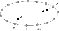
Figure 1: A system of two non-interacting qubits ($A$ and $B$), suffering decoherence from the local interaction with distant sites of an environment chain.

Each of the two qubits in the system interacts locally with a certain spin of the chain: qubit $A$ interacts with spin $0$, and qubit $B$ with spin $d$. The interaction Hamiltonian is:

$$H_{int}=-g(|{1}\rangle\langle{1}|_{A}Z_{0}+|{1}\rangle\langle{1}|_{B}Z_{d})$$ (2)

with $|{0}\rangle$ and $|{1}\rangle$ the two eigenstates of the $Z$ Pauli operator. This has a simple interpretation: the coupling to the qubits induces a change in the effective magnetic field at sites $0$ and $d$. Thus, if the system is in state $|{ab}\rangle$ ($a,b\in\{0,1\}$) the environment evolves with an effective Hamiltonian $H_{ab}$ given by:

$$H_{ab}=H_{C}-g(aZ_{0}+bZ_{d}).$$ (3)

We also assume that the initial state of the “universe” formed by system and environment is of the form:

$$\rho_{SE}(0)=\rho_{0}\otimes|{E_{0}}\rangle\langle{E_{0}}|$$ (4)

where the initial state of the environment $|{E_{0}}\rangle$ is the ground state of the effective Hamiltonian $H_{00}$ Note0 .

Our goal is to study the evolution of $\rho$, the reduced density matrix of the two-qubit system (obtained from the state of the universe by tracing out the environment). Because of the special form of the Hamiltonian, the temporal dependence of $\rho$ can be formally obtained as follows. In the basis of eigenstates of $Z_{A}$ and $Z_{B}$, $\rho$ can be written as:

$$\rho(t)=\sum_{abcd=0,1}\rho_{ab,cd}(t)|{ab}\rangle\langle{cd}|.$$ (5)

The evolution of the matrix elements of $\rho$ is given by:

$$\rho_{ab,cd}(t)=\rho_{ab,cd}(0)\langle{E_{0}}|e^{iH_{cd}t}e^{-iH_{ab}t}|{E_{0}}\rangle$$ (6)

(we take $\hbar=1$). As states in the basis commute with the total Hamiltonian, the diagonal terms $\rho_{ab,ab}$ remain constant. On the other hand, each off-diagonal term in the reduced density matrix is modified by a factor of absolute value between 0 and 1. This factor corresponds to the overlap between two different evolutions of the spin chain. Following LevsteinUP-1998 ; rossini-2007-75 , we denote the square modulus of this factor as the Loschmidt echo:

$$L_{ab,cd}(t)=|\langle{E_{0}}|e^{iH_{cd}t}e^{-iH_{ab}t}|{E_{0}}\rangle|^{2},$$ (7)

which obviously satisfies $L_{ab,cd}=L_{cd,ab}$.

Below, we will show how to compute the echoes $L_{00,ab}$ and $L_{01,10}$. These two echoes are enough to obtain the reduction of the off-diagonal elements in the reduced density matrix when the initial state is one of the four Bell states (or any state satisfying $\rho_{11,01}=\rho_{11,10}=0$). The computation of each of these two echoes is slightly different. In fact, to obtain $L_{00,ab}$ we first note that one of the evolution operators in (7) acts trivially. Therefore, the echo is equal to the survival probability of the initial state after being evolved with the Hamiltonian $H_{ab}$, i.e.

$$L_{00,ab}(t)=\left|\langle{E_{0}}|e^{-iH_{ab}t}|{E_{0}}\rangle\right|^{2}$$ (8)

In turn, the echo $L_{01,10}$ can be calculated noticing that the corresponding effective Hamiltonians are related by a translation:

$$H_{01}=T^{d}H_{10}T^{-d},$$ (9)

where $T$ is the one–site translation operator in the chain. As the ground state of the Hamiltonian $H_{00}$ is an eigenstate of this operator, the echo can be written as:

$$L_{01,10}(t)=\left|\langle{E_{0}}|e^{iH_{10}t}T^{d}e^{-iH_{10}t}|{E_{0}}\rangle\right|^{2}$$ (10)

To obtain the echoes we will make use of the fact that the full quantum evolution for each Hamiltonian $H_{ab}$ can be exactly solved. This can be done by mapping the Hamiltonians $H_{ab}$ of the chain onto a fermion system by means of the Jordan-Wigner transformation LiebSM-1961 :

$$X_{j} = exp\left\{i\pi\sum_{k=1}^{j-1}c_{k}^{\dagger}c_{k}\right\}(c_{j}+c_{j}^{\dagger})$$ (11)

$$Y_{j} = i~{}exp\left\{i\pi\sum_{k=1}^{j-1}c_{k}^{\dagger}c_{k}\right\}(c_{j}-c_{j}^{\dagger})$$ (12)

$$Z_{j} = 2c_{j}^{\dagger}c_{j}-1.$$ (13)

Using this, up to a correction term associated to boundary effects, the Hamiltonians can be written as:

$$H_{ab} = -\sum_{j}\big{\{}(c_{j}^{\dagger}c_{j+1}+c_{j+1}^{\dagger}c_{j})+\gamma(c_{j}^{\dagger}c_{j+1}^{\dagger}+c_{j+1}c_{j})+$$ (14)

$$+\lambda_{j}^{(ab)}(2c_{j}^{\dagger}c_{j}-1)\big{\}}$$

with $\lambda_{j}^{(ab)}=\lambda+g(a\delta_{j,0}+b\delta_{j,d})$ (the extension to qubits interacting with more than one site is trivial).

The Hamiltonians $H_{ab}$ depend quadratically on the annihilation and creation operators. Therefore they can be diagonalized by linear (Bogoliubov) transformations defining new creation and annihilation operators which we will denote as $\eta^{(ab)},\eta^{\dagger(ab)}$. Furthermore, as all these transformations are linear, the operators corresponding to different values of the labels $(ab)$ can also be connected by Bogoliubov transformations.

The echoes we want to compute can be written in terms of the matrices involved in these Bogoliubov transformations. For example, in Appendix A it is shown that:

$$L_{00,ab}(t)=\left|\det({\rm g}+{\rm h}e^{i\Lambda t})\right|^{2}$$ (15)

Here $\Lambda$ is a diagonal $N\times N$ matrix containing the energies of the normal modes of the Hamiltonian $H_{ab}$. ${\rm g}$ and ${\rm h}$ correspond to the transformation connecting the particles that diagonalize the unperturbed Hamiltonian $H_{00}$ and the effective Hamiltonian $H_{ab}$:

$$\eta_{j}^{(00)}=\sum_{k}{\rm g}_{jk}\eta_{k}^{(ab)}+{\rm h}_{jk}\eta_{k}^{\dagger(ab)}$$ (16)

This equation is useful since it expresses the echo as the determinant of an $N\times N$ matrix, which can be efficiently computed (the number of operations is polynomial in $N$). This formula is a new version of the one used in rossini-2007-75 , where the Loschmidt echo was written in terms of the two-point correlators of the environment chain (i.e., as the determinant of a $2N\times 2N$ matrix).

The way to compute the echo $L_{01,10}$ is shown in Appendix B, using the fact that the translation operator $T$ is Gaussian in the fermion operators. The result is, once again, the determinant of an $N\times N$ matrix, though somewhat more complicated:

$$L_{01,10}(t)=\left|\det({\rm g^{\prime}}\tau^{-d}{\rm g^{\prime}}^{\dagger}+{\rm h^{\prime}}\tau^{d}{\rm h^{\prime}}^{\dagger})\right|$$ (17)

Here $\rm{g^{\prime}}$, $\rm{h^{\prime}}$ are time-dependent complex matrices related to Bogoliubov transformations between different sets of particle operators, and $\tau$ is the diagonal matrix expression of the translation operator $T$.

Decoherence for initial states of the form $|\varphi\rangle=\alpha|{00}\rangle+\beta|{11}\rangle$ or $|\varphi\rangle=\alpha|{01}\rangle+\beta|{10}\rangle$ is described by $L_{00,11}$ and $L_{01,10}$ respectively. In any case, the relevant echo $L(t)$ for the Bell-like state $|\varphi\rangle$ will determine not only the process of purity decay but also the way in which the two qubits become disentangled. In fact, if one considers an initial mixture of the form $\rho_{0}=p|{\varphi}\rangle\langle{\varphi}|+(1-p)~{}\mathbb{I}/4$, the purity of the state is the following function of the echo $L(t)$:

$$Tr(\rho^{2}(t))=\frac{1-p^{2}}{2}+p^{2}[1-2|\alpha\beta|^{2}(1-L)].$$ (18)

(here, $L$ is either $L_{01,10}$ or $L_{00,11}$ depending on $|\varphi\rangle$). The entanglement between the two qubits can be measured by the negativity $\mathcal{N}$ obtained from the sum of the negative eigenvalues of the partial transpose of $\rho$ ($\mathcal{N}\neq 0$ is an indicator of non-separability of the two-qubit state) VidalW-2002 . For the mixed initial state proposed:

$$\mathcal{N}(t)=\max\left\{0,p|\alpha\beta|\sqrt{L(t)}-\frac{1-p}{4}\right\}.$$ (19)

For pure initial states ($p=1$), the state is entangled whenever $L\neq 0$; in general, the state becomes disentangled when the echo is below a threshold which depends on $p$. In this way the phenomenon of entanglement sudden death (ESD) may take place yu-2004-93 .

We will analyze the dependence of the echo on the distance between the interaction sites. Two simple limits exist. First, if both qubits couple to the same site ($d=0$) then the echo $L_{01,10}$ becomes trivially 1 as the two effective Hamiltonians are identical. On the other hand, ${L}_{00,11}$ is simply the echo of a single qubit interacting with one site with twice the interaction strength (a case studied in rossini-2007-75 ). The long distance limit is also easy to understand: if the chain is sufficiently large we expect its effect to be equal to the one obtained when each qubit interacts with an independent environment. Then, both ${L}_{00,11}$ and ${L}_{01,10}$ approach ${L}_{0,1}^{2}$ (where ${L}_{0,1}$ is the single-qubit echo). This long distance regime exists only if the back-action of the qubits on the environment is small. For strong back-action, one expects the environment to induce effective interactions between the qubits. As we will see, the long distance limit will be identifiable easily in the weak coupling case, whereas the strong coupling regime will be plagued with effects associated to environment-induced interactions.

III Results: Weak coupling

In this Section we study the case when the coupling $g$ is small compared to the interaction strength between chain sites, showing results for the reference value $g=0.1$. Fig. 2 shows the echo $L_{00,11}$ as a function of time for the Ising chain ($\gamma=1$) and for several values of the transverse field $\lambda$ and the distance $d$. For $\lambda<1$, the echo has small amplitude oscillations (with frequency of order $1$) about a value which is roughly independent of distance. For $\lambda>1$ decoherence is an order of magnitude smaller, oscillations decay rapidly and the echo approaches a constant that grows with distance. In both cases the dependence on distance rapidly saturates: the long distance regime is reached at $d\gtrsim 4$. To the contrary, near the critical point ($\lambda=1$) the echo decreases logarithmically with time (after a short transient), and saturation with distance is not attained, which is a signal of long range correlations in the environment.

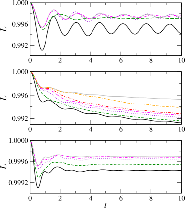
Figure 2: Echo $L_{00,11}$ as a function of time for an Ising chain ($\gamma=1$) of $N=100$ sites weakly coupled to a two–qubit system ($g=0.1$). From top to bottom the transverse field is $\lambda=0.5$, $0.99$, and $1.5$. The distance between qubits is $d=0$ (full black), $1$ (dashed green), $2$ (dotted violet), and $3$ (dash-dotted magenta). In the almost critical case $\lambda=0.99$ we include also $d=4$ ($\cdot\cdot-$, red), and $10$ ($--\cdot$, orange); these curves are not shown in the other plots because they are intertwined with the others. For comparison we display in full grey the limit of two independent environments.

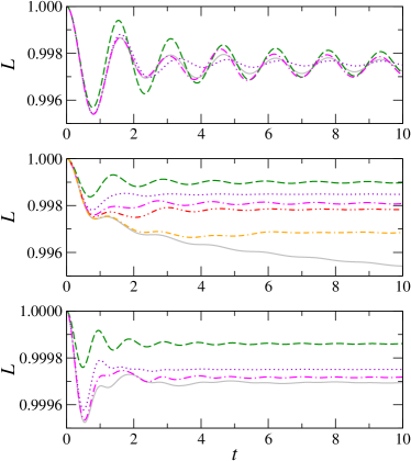
Figure 3: Echo $L_{01,10}$ as a function of time; all parameters are the same as in the previous Figure (for $d=0$ this echo is always equal to 1).

The strongest decoherence is typically obtained at short distances. A simple argument shows that this is reasonable for weak coupling: at short times one expects an approximately Gaussian decay of the echo of the form $\exp(-\alpha^{2}t^{2})$, with $\alpha\propto g$. For $d=0$ we have $\alpha^{2}\sim(2g)^{2}$ while in the case of independent environments $\alpha^{2}\propto 2g^{2}$. As a consequence, faster decay of $L_{00,11}$ is expected for $d=0$ in the weak coupling regime. For the echo $L_{01,10}$ the dependence on distance is opposite to the previous case, as shown in Fig. 3. This is expected since the Hamiltonians $H_{01}$ and $H_{10}$ become more different as $d$ grows. On the other hand, the saturation with distance approaching the limit of independent environments is similar to that of $L_{00,11}(g,t)$.

We analyzed the saturation scale in the following way: we calculated the echo $L_{00,11}$ for $\lambda$ between $0.1$ and $2$, distances $d$ between $1$ and $15$, and times $t_{j}$ in the interval $[0,10]$. The squared norm of the vector obtained substracting the values of the echo at times $t_{j}$ for distance $d$ and for independent environments was taken as a measure of the difference between these echoes. A saturation length $l$ was obtained from the exponential fit of the decay of these norms as $d$ approaches the long distance limit. The behaviour of $l$ as a function of the external field $\lambda$ is shown in Fig. 4. The saturation length was found to be related to the correlation length $\xi=|\ln(\lambda)|^{-1}$ Pfeuty-1970 ; BarouchMcCoy-1971 . Our numerical results indicate that $l\simeq 1.1+0.21*(0.17+\xi^{-1})^{-2.2}$. Indeed, $l$ is clearly increased near the critical point, though it does not diverge like $\xi$. The analysis of the echo $L_{01,10}$ leads to analogous results.

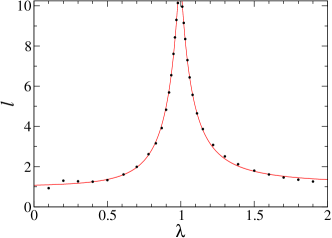
Figure 4: Saturation length as a function of the external field $\lambda$ (dots), for the Ising chain ($\gamma=1$). The continuous red line shows the fit as a function of the correlation length $\xi$ of the chain ($l\simeq 1.1+0.21*(0.17+\xi^{-1})^{-2.2}$). These results correspond to a chain of 500 spins, and the echoes have been smoothed to avoid spurious effects due to oscillations. Besides, the fact that $g>0$ is accounted for by a shift in the correlation length, given by $\xi_{\rm eff}=\xi(\lambda+5.7~{}10^{-3})$.

The echoes obtained for the case $\gamma=0.1$ are qualitatively similar to the ones shown in Figs. 2, 3 for the Ising chain. There are nevertheless some noticeable differences. These concern mainly the dependence on distance, which is rather irregular for $\lambda\leq 1$. Besides, the connection between the saturation distance $l$ and the correlation length $\xi$ is not evident, even though the saturation length clearly increases in the proximity of the critical point. There are also differences in the shape of the decay close to criticality (almost linear for times up to $t\sim 10$), and in the strength of the decoherence process (for $\lambda\leq 1$ decoherence is stronger than in the case $\gamma=1$, while for $\lambda>1$ it is weaker).

The previous results refer to times shorter than the ones where the finite size of the environment starts to play a role. For long times finite size effects become important, as shown by the coherence revivals and sharp decays of Fig. 5. These imply that the qubits are not independent due to environment–induced interactions. By decreasing $d$ below $N/4$ the first peak or decay tends to disappear, so that the qubits evolve almost independently even for long times (provided $d$ is over the saturation scale). This will not be the case in the strong coupling regime, which will be treated in the next section.

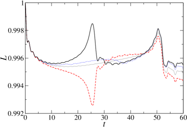
Figure 5: The echo for two qubits weakly interacting with a spin chain of $N=100$ sites has revivals or sharp decays due to finite-size effects. For a distance $d=N/2$ we show $L_{00,11}$ (full black) and $L_{01,10}$ (dashed red). When $d$ decreases the first peak/decay tends to dissappear (the dotted blue line corresponds to $L_{00,11}$ for $d=30$). The result for two qubits coupled to independent environments is shown for comparison (full grey). The parameters are $\lambda=0.99$, $\gamma=1$, $g=0.1$.

IV Results: Strong coupling

For strong system-environment coupling, the results are quite different from the ones above. As observed for a single spin system in cucchietti-2006 ; CormickP-2007 , the strong coupling regime is characterized by an echo with a fast oscillation and a slow envelope which for large enough $g$ is independent of $g$. Following the same steps as in CormickP-2007 we can explain the behaviour of the echo $L_{00,11}$ as follows: Consider the evolution with Hamiltonian $H_{11}=H_{00}-g(Z_{0}+Z_{d})$. As all the frequencies associated with the interaction Hamiltonian are of order $g$ (much larger than typical frequencies of the chain), we may approximate:

$$e^{-iH_{11}t}|{E_{0}}\rangle\simeq e^{igt(Z_{0}+Z_{d})}e^{-itH^{\prime}}|{E_{0}}\rangle.$$ (20)

Here $H^{\prime}$ is the Hamiltonian $H_{00}$ reduced to a block diagonal form, with blocks associated with the different eigenvalues of the interaction term. The evolution operator thus factors in two parts: a fast periodic evolution with frequency of order $g$, and a slow evolution that determines the envelope of the echo and is governed by an effective chain Hamiltonian $H^{\prime}$ (which does not depend on $g$). This same argument can be adapted to $L_{01,10}$. We note, however, that this behaviour is a consequence of the form of the interaction between system and environment and is not generic for strong couplings. For instance, if each qubit interacts with a region of the chain with a coupling that decreases with distance, the typical result is a sudden decay of coherence without oscillations.

For strong coupling we expect decoherence to increase with distance (until saturation) for both echoes. Indeed, for $d=0$ we have $L_{00,11}(g,t)=L_{0,1}(2g,t)$, with $L_{0,1}$ the single qubit echo. This must be of the same order as $L_{0,1}(g,t)$ because for large enough $g$ the envelope is independent of $g$. On the other hand, in the long distance limit $L_{00,11}(g,t)\simeq L_{0,1}^{2}(g,t)$, which is smaller than $L_{0,1}(g,t)$. The comparison between $d\gg 1$ and $d=0$, illustrated in Fig. 6 for $\gamma=1$, $\lambda=0.99$, thus leads to a result which is quite the opposite of the one obtained for weak coupling. The distance dependence of the echo $L_{01,10}$ follows a similar pattern, i.e., decoherence increases with distance, as shown in Fig. 7.

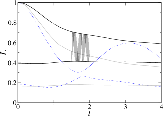
Figure 6: Envelope of the echo $L_{00,11}$ as a function of time for two qubits strongly interacting with two different sites of a chain with $N=100$, $\lambda=0.99$, $\gamma=1$, $g=50$. The plots correspond to the cases of distance $d=0$ (full black), 2 (dotted blue), and long-distance limit (full grey). For the case $d=0$ a part of the fast oscillation is included. Here, in contrast to the weak coupling scenario, decoherence is stronger in the long distance limit, as the envelope for large $d$ corresponds to the square of the one for $d=0$.

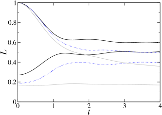
Figure 7: Envelope of the echo $L_{01,10}$ as a function of time for two qubits strongly interacting with two different sites of a chain with $N=100$, $\lambda=0.99$, $\gamma=1$, $g=50$. The plots correspond to the cases of distance $d=1$ (full black), 2 (dotted blue), and long-distance limit (full grey). For the case $d=0$ there is no decoherence in this case, while for $d\geq 1$ decoherence turns out to be stronger as distance is increased.

Environment–induced interactions between qubits are manifest in Fig. 6. Indeed, for $d>0$ appart from the fast oscillation with a decaying envelope the echo $L_{00,11}$ exhibits a beating (or revival) at a time that depends on $d$. This effect is not important for weak coupling and can be interpreted as due to the interaction between the qubits through the modes of the perturbed chain. On the contrary, no revivals are seen for $L_{01,10}$.

The difference can be understood by analyzing the origin of revivals in terms of the spectrum of the Hamiltonian and the Bogoliubov coefficients, contained in the matrices $\Lambda$, $\rm g$ and $\rm{h}$ in (15). Excitations of the unperturbed Hamiltonian have energies lying between $2|1-\lambda|$ and $2|1+\lambda|$. When a strong external field is applied in two sites, two eigenvalues of order $g$ appear; these excitations are associated to combinations of the original fermion operators in the two sites. The remaining excitations (with eigenvalues of the same order as before) can be split in two groups, corresponding roughly to excitations between and outside the interaction sites (this labelling only makes sense because we consider distances $d\ll N$). It turns out that the most populated levels correspond to the lowest energy excitation (occupying the outside region), the excitations in the interaction sites, and those lying in the inside region Note1 . The high–energy excitations are associated to the rapid echo oscillation, while the lowest energy excitation has a time scale growing with $N$. The beating in the echo is given by the lowest-energy mode in the region between the qubits.

The situation for $L_{01,10}$ is different, as seen in Fig. 7, because for each effective Hamiltonian there is a single site perturbation of the chain. In this case the chain cannot be split in two regions and the populations of the low-energy levels decrease slowly with the energy, in such a way that there is not a single frequency associated to them. Then, no revivals occur up to times long enough for finite-size effects to appear.

The revivals for the case $L_{00,11}$ appear for $\lambda<1$ but not for $\lambda>1$. This is a consequence of the change in the properties of the chain. Indeed, for $\lambda<1$ the revival time is shorter as $\lambda$ is increased because the lowest energy associated to excitations between the qubits increases. For $\lambda>1$, the dissappearance of the revivals may be related to the fact that many low-energy excitations become populated, with frequencies comparable to the one associated to the beating.

The first revival time, $t_{r}$, and the amplitude of the peak, $L_{r}$, can be analyzed as functions of the distance $d$. We consider first a critical case where $H_{00}$ and $H_{11}$ belong to different phases ($\lambda=0.99$, $\gamma=1$, $N=100$). In each case, new peaks appear at multiples of $t_{r}$. For $d>1$, the revival time grows linearly with distance ($t_{r}\approx 2d$), while $L_{r}$ decays as a power law, $L_{r}\propto d^{-1/4}$. For distances $d\gtrsim N/5$ effects associated with the finite size of the chain appear altering the regular trend. Examining the echo for $\lambda$ far away from the phase transition we found a slower decay of the revival peak with $d$. Furthermore, in this case $t_{r}$ is not linear with $d$, but seems to grow exponentially. Thus, $t_{r}$ appears to be related to transport properties of the chain that are modified by varying the external field. This should serve as a warning not to picture revivals as the manifestation of a spin wave propagating with constant velocity along the chain (the energies of the lowest modes between the qubits do not generally scale as $1/d$).

Changing the anisotropy parameter $\gamma$, the envelopes display different shapes, heights and revival times. The distance dependence of the revival time $t_{r}$ and amplitude $L_{r}$ was studied for $\lambda=0.99$ and $\gamma$ between $0.1$ and $1$. We found that $t_{r}$ generally grows as a power law. Besides, the height of the revival peaks decreases with increasing $\gamma$, and the dependence of $L_{r}$ with $d$ maintains a power-law decay. We note, however, that the peaks lose definition for large $d$ and small $\gamma$.

V Conclusions

We studied the evolution of a system of two qubits interacting locally with an XY chain. Decoherence and disentanglement are determined by a Loschmidt echo, which we computed using previous results rossini-2007-75 ; cozzini-2006 . The formulas we obtained for the echoes enabled us to study a family of initial states including the four Bell states. We focused our analysis on the dependence of the echo with the distance between the interaction sites. The cases we studied show a rich variety of results. For instance, for strong coupling decoherence increases with increasing distance for all Bell states. On the contrary, for weak coupling decoherence may increase or decrease with distance according to the initial state chosen.

In the regime of weak system–environment coupling the dependence of the echo with distance saturates very fast except for the critical case. The saturation length $l$ characterizing the approach to the long distance limit seems to depend on the correlation length of the chain $\xi$. This result is interesting as it relates an equilibrium quantity (the correlation length $\xi$) with a dynamical quantity $l$. However, this relation was only found for the Ising case, and will be further analyzed elsewhere.

The strong coupling regime is characterized by fast oscillations with a slowly decaying envelope. For some initial states, this envelope shows a beating which can be interpreted as an interaction of the qubits through the chain. Its time scale is determined by the modes of the chain in the region between the qubits, which depend on the distance between them and on the values of the parameters in the chain Hamiltonian (indeed, the beatings were found only for $\lambda<1$). We note that in this regime the fast oscillation of the echo continually provokes decays and revivals of the entanglement between qubits. This is just a dynamical transfer of this entanglement back and forth from the system to its immediate vicinity with a frequency given by the coupling constant $g$. The true loss of entanglement is produced by the decay of the oscillation. If the initial state is mixed, this decay can lead to true sudden death of entanglement. When the distance between qubits is short, the sudden death may be followed by a sudden revival due to the beating in the echo. For very long distances, entanglement loss becomes irreversible, unless we consider times which are long enough for the finite size of the environment to become manifest.

Finally, it is worth pointing out that there are formal analogies between the model we solved and other decoherence models. In fact, decoherence for two qubits at distance $d$ in an initial state of the form $\alpha|{00}\rangle+\beta|{11}\rangle$ is identical to that of a single qubit interacting non-locally with sites $0$ and $d$ (which was partially studied in rossini-2007-75 ). On the other hand, for the case of states of the form $\alpha|{01}\rangle+\beta|{10}\rangle$, the relevant echo $L_{01,10}$ can be mapped onto the one of another equivalent problem: a spinless particle occupying discrete positions along the chain (with position eigenstates $|{x_{j}}\rangle$, $j=0,\ldots,N-1$). If this particle modifies the effective magnetic field for the spin in the site it occupies, cat states of the form $(|{x_{j}}\rangle+|{x_{j+d}}\rangle)/\sqrt{2}$ will decohere as a consequence of the interaction. The resulting reduction of the off-diagonal terms will be precisely given by expression (17).

Note added: After the submission of this paper, we became aware of the work in rossini-2008-77 , which shows how to calculate efficiently the remaining elements of the density matrix ($\rho_{01,11}$).

VI Appendix A

In this section we show how the formula (15) for the echo can be obtained. Taking into account the relation (16) between the operators that diagonalize the different effective Hamiltonians,

$$\eta_{j}^{(0)}=\sum_{k}{\rm g}_{jk}\eta_{k}^{(1)}+{\rm h}_{jk}\eta_{k}^{\dagger(1)}$$

the two vacuum states $|{E_{0}}\rangle$ (for the unperturbed Hamiltonian) and $|{E_{0}^{\prime}}\rangle$ (for the perturbed one) can be connected by chung-2001-64 :

$$|{E_{0}}\rangle\propto\exp\left\{\frac{1}{2}\vec{\eta}^{\dagger(1)}G\vec{\eta}^{\dagger(1)}\right\}|{E_{0}^{\prime}}\rangle$$ (21)

with $G=-{\rm g}^{-1}{\rm h}$ (for the sake of simplicity, we shall first assume that $\rm{g}$ is invertible, and sketch the most general case afterwards). The echo can then be calculated from:

$$L(t) = |\langle{E_{0}}|e^{-iH_{1}t}|{E_{0}}\rangle|^{2}$$ (22)

$$\propto |\langle{E_{0}^{\prime}}|e^{-\frac{1}{2}\vec{\eta}G^{*}\vec{\eta}}e^{-it\vec{\eta}^{\dagger}\Lambda\vec{\eta}}e^{\frac{1}{2}\vec{\eta}^{\dagger}G\vec{\eta}^{\dagger}}|{E_{0}^{\prime}}\rangle|^{2}$$

where in the last expression $\Lambda$ is a diagonal matrix containing the energies corresponding to the different particles, and all super-indices are omitted as all operators and matrices refer to the perturbed Hamiltonian $H_{1}$. By introducing two identities in terms of fermionic coherent states between the exponentials and integrating two times, NegeleO-1987 we obtain:

$$L(t) \propto \Bigg{|}\int d\alpha_{1}\ldots d\alpha_{N}d\beta_{1}\ldots d\beta_{N}$$ (23)

$$\exp\left\{\frac{1}{2}\vec{\alpha}G^{*}\vec{\alpha}+\vec{\beta}e^{it\Lambda}\vec{\alpha}-\frac{1}{2}\vec{\beta}G\vec{\beta}\right\}\Bigg{|}^{2}$$

where $\vec{\alpha},\vec{\beta}$ are Grassman $N$-tuples. This is a Gaussian integral, that can be solved to:

$$L(t)\propto\left|\det\begin{pmatrix}G^{*}&-e^{it\Lambda}\\ e^{it\Lambda}&-G\end{pmatrix}\right|$$ (24)

Using properties of the determinant and the fact that $\Lambda$ is diagonal, and imposing that $L(0)=1$ the echo can be rewritten as:

$$L_{01,10}(t)=\left|\det({\rm g}e^{it\Lambda}{\rm g}^{\dagger}+{\rm h}e^{-it\Lambda}{\rm h}^{\dagger})\right|$$ (25)

The formula can be simplified further: since $\rm{g}$, $\rm{h}$ are real we have that $\rm{g}\pm\rm{h}$ is orthogonal, and using this we obtain the final expression (15):

$$L(t)=\left|\det({\rm g}+{\rm h}e^{i\Lambda t})\right|^{2}$$

In case $\rm{g}$ is not invertible, the relation (21) between the vacuum states can be generalized by using intermediate sets of operators cozzini-2006 . By the singular value decomposition, ${\rm g}=UDV$ with $D$ diagonal, $U,V$ orthogonal. We define new fermionic operators $\vec{\xi}_{j}^{(0)}=U^{t}\vec{\eta}^{(0)}$, $\vec{\xi}^{(1)}=V\vec{\eta}^{(1)}$. The linear transformation between the $\xi^{(i)}$, $\xi^{\dagger(i)}$ now has $D$ instead of $\rm{g}$, and the vacuum states are the same because the transformation does not mix creation and annihilation operators. We can assume $D_{j}=0$ for $j\leq j_{1}$, and the remaining eigenvalues to be nonzero. By interchanging particles with holes ($\xi_{j}^{(0)}\leftrightarrow\xi_{j}^{\dagger(0)}$) for every index such that $D_{j}=0$ we obtain a linear transformation with an invertible matrix. The calculation of the echo follows the same steps as before, except that it is necessary to treat indices $j\leq j_{1}$ separately. After the Gaussian integration, we are left with an expression of the form (24) in which only indices $j>j_{1}$ appear. The desired result can be achieved by conveniently introducing some rows and columns in the matrix, in such a way to include the parts of the matrices with $j\leq j_{1}$ without changing the value of the determinant.

The present derivation cannot be easily extended to more general cases, with two different evolution operators as in (7), for in that case there are three sets of operators that must be related. The steps taken in the calculation above then lead to a result that involves a sum over an exponential number of terms, and so cannot be efficiently evaluated.

VII Appendix B

Here we sketch the derivation of the formula (17) for the decay of the off-diagonal terms $\rho_{01,10}$. We start from expression (10), which involves two sets of particle operators: one which we note as $\eta^{(1)}$, diagonalizing the effective Hamiltonian $H_{10}$, and the set $\eta^{(0)}$ for the unperturbed chain Hamiltonian $H_{00}$. These two sets are connected by a real Bogoliubov transformation.

The translation operator can then be written as Note2 :

$$T=e^{\frac{2\pi i}{N}\sum_{k=1}^{N}k\eta^{(0)\dagger}_{k}\eta^{(0)}_{k}}$$ (26)

so that the echo is given by:

$$L_{01,10}(t)=\left|\langle{E_{0}}|e^{\frac{2\pi i}{N}\sum_{k=1}^{N}k\alpha^{\dagger}_{k}\alpha_{k}}|{E_{0}}\rangle\right|^{2}$$ (27)

with

$$\alpha_{k}=e^{iH_{10}t}\eta^{(0)}_{k}e^{-iH_{10}t}.$$ (28)

This leads us to an echo of exactly the same form as that in Appendix A, except that the energy matrix $\Lambda$ is replaced by a matrix with the eigenvalues of the translation operator, and the set of particles $\eta^{(1)}_{k}$ is replaced by the $\alpha_{k}$. The main difference here is given by the fact that the Bogoliubov transformation between the $\alpha_{k}$ and the $\eta^{(0)}_{k}$ has time-dependent complex coefficients:

$$\eta_{j}^{(0)}=\sum_{k}{\rm g^{\prime}}_{jk}\alpha_{k}+{\rm h^{\prime}}_{jk}\alpha_{k}^{\dagger}$$ (29)

with

$${\rm g^{\prime}} = {\rm g}e^{it\Lambda}{\rm g}^{t}+{\rm h}e^{-it\Lambda}{\rm h}^{t},$$ (30)

$${\rm h^{\prime}} = {\rm g}e^{it\Lambda}{\rm h}^{t}+{\rm h}e^{-it\Lambda}{\rm g}^{t}.$$ (31)

Following steps similar to those in Appendix A, we finally obtain for the echo the expression (17):

$$L_{01,10}(t)=\left|\det({\rm g^{\prime}}\tau^{-d}{\rm g^{\prime}}^{\dagger}+{\rm h^{\prime}}\tau^{d}{\rm h^{\prime}}^{\dagger})\right|$$

where the diagonal matrix $\tau$ contains the eigenvalues of the translation operator $T$; the structure is the same as in (25). In this way the decay of the off-diagonal terms can once more be written as the determinant of an $N\times N$ matrix. This expression is not as simple as the final one obtained in Appendix A; the reason for this is that the matrices $\rm{g}\pm\rm{h}$ were orthogonal, while the matrices $\rm{g^{\prime}}\pm\rm{h^{\prime}}$ do not satisfy a similar condition.

References

- (1) H. D. Zeh. Found. Phys., 3:109 (1973).
- (2) J.P. Paz and W.H. Zurek. In Coherent Atomic Matter Waves, Les Houches Session LXXII, edited by R. Kaiser, C. Westbrook, and F. David (Springer-Verlag, Berlin, 2001), p. 533-614.
- (3) W.H. Zurek. Rev. Mod. Phys., 75:715–775 (2003).
- (4) M. A. Nielsen and I. L. Chuang. Quantum computation and quantum information. Cambridge University Press, Cambridge, U.K. (2000).
- (5) C. Cormick and J. P. Paz. Phys. Rev. A 77, 022317 (2008)
- (6) J. Jing and Z.-G. Lu. ArXiv e-print quant-ph/0612115 (2006).
- (7) T. Yu and J. H. Eberly. Phys. Rev. Lett., 93:140404 (2004).
- (8) We avoid taking values of the Hamiltonian parameters for which the ground state is undefined because of degeneracy.
- (9) D. Rossini, T. Calarco, V. Giovannetti, S. Montangero, and R. Fazio. Phys. Rev. A, 75:032333 (2007).
- (10) P. R. Levstein, G. Usaj, and H. M. Pastawski. J. Chem. Phys. 108:2718 (1998).
- (11) E. Lieb, T. Schultz, and D. Mattis. Ann. of Phys., 16:407–466 (1961).
- (12) G. Vidal and R. F. Werner. Phys. Rev. A, 65(3):032314 (2002).
- (13) P. Pfeuty. Ann. of Phys., 57:79–90 (1970).
- (14) E. Barouch and B. Mc Coy. Phys. Rev. A, 3(2):786–804 (1971).
- (15) F. M. Cucchietti, S. Fernandez-Vidal, and J. P. Paz. Phys. Rev. A, 75:032337 (2007).
- (16) The populations of the particles that diagonalize the perturbed Hamiltonian in the ground state of the unperturbed chain are .
- (17) M. Cozzini, P. Giorda, and P. Zanardi. Phys. Rev. B, 75:014439 (2007).
- (18) M.-C. Chung and I. Peschel. Phys. Rev. B, 64:064412 (2001).
- (19) J. W. Negele and H. Orland. Quantum many-particle systems, volume 68 of Frontiers in Physics. Addison-Wesley, Redwood City, CA (1987).
- (20) D. Rossini, P. Facchi, R. Fazio, G. Florio, D. A. Lidar, S. Pascazio, F. Plastina, and P. Zanardi. Phys. Rev. A, 77:052112 (2008).
- (21) For numerical computations, we use an auxiliary basis given by the Fourier transform of the operators . This basis diagonalizes naturally the translation operator.