Sensitivity and spatial resolution of square loop SQUID magnetometers

Abstract

We calculate the flux threading the pick-up coil of a square SQUID magnetometer in the presence of a current dipole source. The result reproduces that of a circle coil magnetometer calculated by Wikswo [1] with only small differences. However it has a simpler form so that it is possible to derive from it closed form expressions for the current dipole sensitivity and the spatial resolution. The results are useful to assess the overall performance of the device and to compare different designs.

1 Introduction

The application of Superconducting QUantum Interference Devices (SQUIDs) to the measurement of biomagnetic fields has occurred because of their sensitivity, their stability and their flexibility. In fact SQUID based devices offer the possibility to implement measurements where no other methodology is possible and moreover they present the advantage to be a non-invasive technique [2], [3]. Usually studies, aimed to develop better devices, focus on gradiometric configurations since they are less sensitive to the noise. Hereafter we focus on magnetometer configuration which is successfully employed in multichannel systems for biomagnetic imaging [4]. Magnetometers are extremely sensitive to the outside environment, while some other configuration, like gradiometers provide the advantage of discriminating against unwanted background fields from distant sources while retaining sensitivity to the nearby sources.
In a dc-SQUID magnetometer, the pick-up coil, collects the magnetic flux giving an effective area much larger than that of the SQUID itself [5]. Here we study the effect of magnetometer pick-up coil geometry on the performances of SQUID devices for biomagnetism. Well known and widely spread expressions for the flux threading a magnetometer and the current dipole sensitivity have been calculated by Wikswo [1] referring to a circular loop device. Since typically, SQUID magnetometers present a square pick-up loop [5], we were driven, for the best characterization of such devices, but also for general reasons, to recalculate the quantities of interest in the case of square pick-up loop. It turned out that expressions for the minimum detectable current dipole and for the spatial resolution are easily derived for the square geometry.

2 Magnetic flux threading a square magnetometer in the current dipole model

A widely used mathematical model to describe bioelectric currents is the current dipole [6]. It is a good model of elementary cellular events, thus it can be used for magnetoencephalography as well for magnetocardiography studies.
Let us consider a dipolar electric current source $\vec{p}\left(p_{x},p_{y}\right)$ located at a point $\vec{r^{\prime}}=(x^{\prime},0,z^{\prime})$ in a conducting half space and a pick-up loop centered on the z-axis (Fig.1). The magnetic field generated by the source $\vec{p}$ at a point $\vec{r}=(x,y,z)$ has the vector potential $\overrightarrow{A}({A_{x},A_{y},0})$

$$A_{x,y}=\frac{\mu_{0}p_{x,y}}{4\pi\sqrt{\left(x-x^{\prime}\right)^{2}+\left(y-y^{\prime}\right)^{2}+\left(z-z^{\prime}\right)^{2}}}$$ (1)

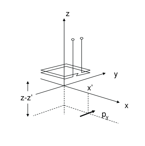
Figure 1: Schematic of the square loop magnetometer. A current dipole source $\vec{p}$ is placed at the point $\vec{r^{\prime}}=(x^{\prime},0,z^{\prime})$.

By using eq.(1) it is possible to calculate the magnetic flux through the considered pick-up coil by performing a line integral around the loop. In the case of a circular loop having radius $R$, Wikswo [1] derived the result

$$\Phi=\frac{\mu_{0}p_{y}}{k\pi}\sqrt{\frac{R}{x^{\prime}}}\left[\left(1-\frac{k^{2}}{2}\right)K(k)-E(k)\right]$$ (2)

where

$$k^{2}=\frac{4x^{\prime}R}{\left[(x^{\prime}+R)^{2}+(z-z^{\prime})^{2}\right]}$$ (3)

$K(k)$ and $E(k)$ are respectively the complete elliptic integrals of first and second kind. In a very similar way we have calculated the flux collected by a square loop magnetometer having size $L$, laying parallel to the $xy$ plane, at a distance $D=z-z^{\prime}$ above a current dipole source $\vec{p}$ (Fig.1). The result is

$$\Phi=\frac{\mu_{0}p_{y}}{2\pi}\left[\sinh^{-1}\left(\frac{L}{\sqrt{4D^{2}+(L-2x^{\prime})^{2}}}\right)-\sinh^{-1}\left(\frac{L}{\sqrt{4D^{2}+(L+2x^{\prime})^{2}}}\right)\right]$$ (4)

Note that $p_{x}$ does not contribute to the collected flux for symmetry reasons, so that there is no loss of generality if we consider $\vec{p}$ as having only the $y-$component. In order to compare devices presenting different geometries (square loop or circle loop), we shall consider equal area devices, that is equivalent to the condition $R=L/\sqrt{\pi}$. Also we shall introduce in the above equations the dimensionless source position $\overline{x}=x^{\prime}/D$, the reduced flux $\Phi\pi/\mu_{0}p_{y}$ and the geometrical parameter $q=L/D$. As we shall see, although eq.(2) and eq.(4) give, almost, the same result, eq.(4) allows for useful analytical progresses which eq.(2) does not permit.

3 Maximum magnetic flux

In order to evaluate the minimum detectable current dipole and the spatial resolution as a function of the geometrical parameters $L$ and $D$, it is essential to determine the value of the maximum flux and the maximizing source position $x^{\prime}=x^{\prime}_{max}$ for any $q$.
In Fig.2 the reduced flux, calculated by means of eqs.(2), (4), is plotted as a function of the reduced source position $\overline{x}$ for two different values of the ratio $q$, for the two geometries, circle and square. As a general picture one sees that the flux is zero when the source is exactly under the loop ($x^{\prime}=0$) and, as the source moves away, it maximizes for $x^{\prime}=x^{\prime}_{max}$, before decaying out.
While the elementary procedure (zeros of the derivatives) for the maximum finding does not give straightforward results for eq.(2) and eq.(4), simple approximate analytical results can be obtained for the maximum flux, on the basis of physical considerations. First consider the case of a large loop size to source distance ratio ($q\gg 1$). It is evident that in this case (in exact manner in the limit of zero distance) the collected flux is maximum when the source position coincides with the loop edge. This is to say $x^{\prime}=L/2$ ($\overline{x}=q/2$) and $D\rightarrow 0$ for a square loop, and analogously, $x^{\prime}=R$ ($\overline{x}=q/\sqrt{\pi}$) and $D\rightarrow 0$ for a circle loop. Thus we can take this asymptotic values, $q/2$ and $q/\sqrt{\pi}$, as approximate maximum positions for the circle and the square loop, as it is shown in Fig.2, where the two maxima correspond roughly to the points $\overline{x}=2.5$ and $\overline{x}=2.82$ respectively, since q=5 for the curves in Fig.(2).
In the case of a square loop, using the value $q/2$ in eq.(4), we are lead to the following result for the maximum flux

$$\Phi_{max}^{square}=\frac{\mu_{0}p_{y}}{2\pi}\left[\sinh^{-1}\left(\frac{q}{2}\right)-\sinh^{-1}\left(\frac{q}{\sqrt{4+4q^{2}}}\right)\right]$$ (5)

Now we turn to the case when the ratio between the loop size and the distance is quite small ($q\ll 1$). Equations (2) and (4) give in practice identical results for the two loop geometries and the difference between the fluxes threading devices with different shape cannot be appreciated: the two results overlap.
For large distances above the source, or small loop area, equations (2),(4) can be simplified by substituting $R=L/\sqrt{\pi}$ in eq.(2), and then expanding these expressions in the small parameter $q$. Both equations give the same result

$$\Phi=\frac{{\mu_{0}p_{y}}}{4}\frac{\overline{x}}{\left(1+\overline{x}^{2}\right)^{3/2}}\left(\frac{L}{D}\right)^{2}=\frac{{\mu_{0}p_{y}}}{4\pi}\frac{\overline{x}}{\left(1+\overline{x}^{2}\right)^{3/2}}\left(\frac{R}{D}\right)^{2}$$ (6)

which is shown in Fig.2 by the gray curves on the left, calculated for $q=0.5$.

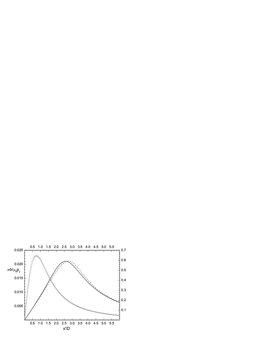
Figure 2: Comparison between the normalized flux threading devices presenting square or circle shape as a function of the source position $x^{\prime}/D$. Gray curves on the left have been obtained using $q=0.5$ in eq.(4). The two black curves on the right have been obtained using $q=5$ in eq.(4). The gray dotted curve shown on the left has been obtained by using for both geometries the Taylor expansion, given by eq.(6).

thus eq.(6) represents the flux as a function of $\overline{x}$, threading a magnetometer positioned at large distance, with respect to the loop size, above the source. In Fig.2 the dotted curve represents results obtained by eq.(6). In this regime ($q\ll 1$) circle and square loop, give identical results, so that any information about the shape of the magnetometer loop is lost. It is easily found that eq.(6) maximizes exactly for $\overline{x}=\frac{\sqrt{2}}{2},(x^{\prime}=\frac{\sqrt{2}}{2}D)$ so that the maximum flux, for small loop size to source distance ratio ($q\ll 1$) is

$$\Phi_{max}=\left(\frac{L}{D}\right)^{2}\frac{\mu_{0}p_{y}}{6\sqrt{3}}=\left(\frac{R}{D}\right)^{2}\frac{\pi\mu_{0}p_{y}}{6\sqrt{3}}$$ (7)

Thus small differences in the collected flux, due to the inhomogeneity of the source, emerge between square and circle geometry only when the source is close faced to the loop. This situation is illustrated in Fig.2 by the black curves on the right, calculated for $q=5$. As can be seen, the two curves maximize in slightly different points, as already observed.
A quantitative evaluation, based on numerics, of the validity of the approximations given by eq.(5) and eq.(7) as well as of the maximizing positions will be given in the next section. We close this section by an estimation of the maximum flux for a typical situation. If we consider for the current dipole the value $p_{y}=10nA\cdot m$ we find that $\Phi^{square}_{max}=9.18\cdot 10^{-17}$ Wb $\cong 45$ m$\Phi_{0}$ for $q=0.5$ (obtained by using the values $L=9$ mm, $D=1.8$ cm).

4 Minimum detectable current dipole

In order to determine the smallest detectable current dipole $p_{y}^{min}$, we have to impose that the collected flux $\Phi_{max}^{square}$ is comparable to the total flux noise $\Phi^{*}$. Therefore $p_{y}^{min}$ is an evaluation for the sensitivity of the considered device: if a device can detect a smaller $p_{y}$, then it presents a higher sensitivity.
For large $q$ values ($q\gg 1$), from eq.(5) for $\overline{x}=q/2$ we obtain

$$p_{y}^{min}=\frac{2\pi\Phi^{*}}{\mu_{0}}\left[\sinh^{-1}\left(\frac{q}{2}\right)-\sinh^{-1}\left(\frac{q}{\sqrt{4+4q^{2}}}\right)\right]^{-1}$$ (8)

For small $q$, from eq.(7) we obtain

$$p_{y}^{min}=\frac{6\sqrt{3}\Phi^{*}}{\mu_{0}q^{2}}$$ (9)

The dependence of the sensitivity on the loop to source distance ratio described by eqs.(8), (9) is shown in Fig.3. In the same figure it is also shown for a comparison, $p_{y}^{min}$ evaluated by a numerical maximum finding procedure directly from eq.(4).
For very small loop size to source distance ratio ($q->0$) the current dipole sensitivity diverges as $q^{-2}$, due to the small area of the SQUID pick-up loop. In the opposite limit, i.e. for very small distance between source and sensor or very large SQUID sensors ($q->\infty$), the sensitivity improves without limits ($p_{y}->\infty$) because the collected flux continues to grow.

5 Spatial resolution

When the current dipole source moves from the position of the maximum flux along the $x$ direction, with a displacement $\delta$, there is a change in the flux $\Delta\Phi$. In a general way, for small $\delta$, one obtains the following expression

$$\Delta\Phi=\Phi(x^{\prime})|_{x^{\prime}_{max}+\delta}-\Phi(x^{\prime})|_{x^{\prime}_{max}}=$$

$$\left(\Phi(x^{\prime})|_{x^{\prime}_{max}}+\frac{\Phi^{\prime\prime}}{2}|_{x^{\prime}_{max}}\delta^{2}\right)-\Phi(x^{\prime})|_{x^{\prime}_{max}}=\frac{\Phi^{\prime\prime}}{2}|_{x^{\prime}_{max}}\delta^{2}$$ (10)

where $x^{\prime}_{max}$ is the value for which the flux maximizes and the condition $\Phi^{\prime}(x^{\prime}_{max})=0$ has been used.
If we now assume that the spatial resolution is “the least detectable displacement” corresponding to a variation in flux equal to the flux noise $\Phi^{*}$, by inverting eq.(5) one obtains

$$\delta^{2}=\frac{2\Phi^{*}}{|\Phi^{\prime\prime}(x^{\prime}_{max})|}$$ (11)

The smaller is $\delta$, the better is the resolution.

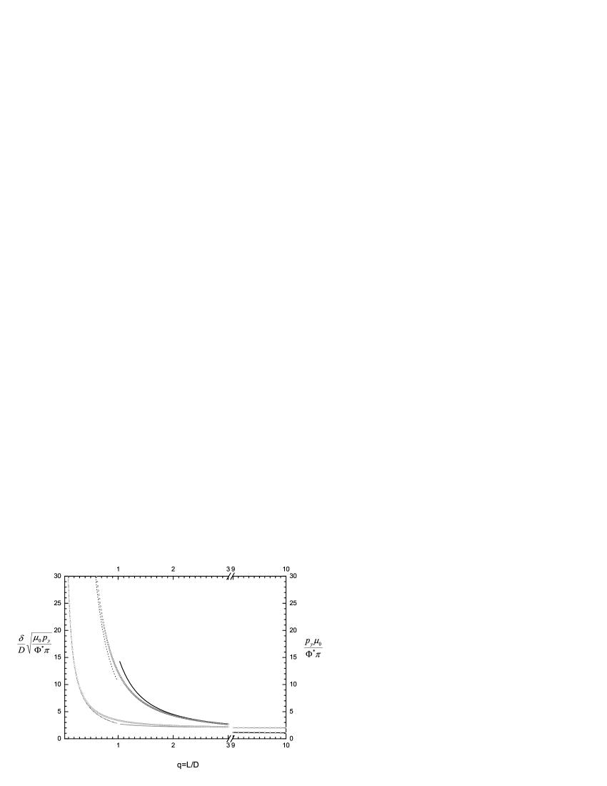
Figure 3: The spatial resolution and the current dipole sensitivity versus the ratio of the side of a square sensor to the source-sensor distance. Black curves describe the current dipole sensitivity: solid curve is for the case $q\gg 1$ (eq.8), dotted curve is for the case $q\ll 1$ (eq.8) and circles are for the numerical calculation. Gray curves describe the spatial resolution: solid curve is for the case $q\gg 1$ (eq.12), dashed curve is for the case $q\ll 1$ (eq.13) and squares are for the numerical calculation.

We now derive an analytical expression for the spatial resolution. For large loop size to source distance ratio ($q\gg 1$), as we have seen before, the flux maximizes approximatively when the condition $x^{\prime}_{max}(q)=q/2$ is satisfied. In this regime, the expression derived for spatial resolution from eqs.(4), (11), developed around $\overline{x}=\frac{q}{2}$, becomes

$$\overline{\delta}=\frac{\delta}{D}=\frac{\sqrt{\frac{\Phi^{*}\pi}{\mu_{0}p_{y}}}}{\sqrt{q\left(\frac{1}{4\sqrt{\left(4+q^{2}\right)}}-\frac{1-\frac{3}{4}q^{2}-\frac{9}{8}q^{4}}{\left(1+q^{2}\right)^{2}\left(4+5q^{2}\right)^{3/2}}\right)}}$$ (12)

For small loop to source distance ratio ($q\ll 1$), the analytical expression for the spatial resolution can be obtained on the basis of eqs.(6) and (11), for $\overline{x}=\frac{\sqrt{2}}{2}$, and the expression for spatial resolution is

$$\overline{\delta}=\frac{\delta}{D}=\frac{3}{q}\sqrt{\frac{\sqrt{3}}{2}\frac{\Phi^{*}\pi}{\mu_{0}p_{y}}}$$ (13)

When the $q$ value is about 1, the approximations introduced till for $\overline{\delta}$ now begin to fail, so that it is necessary to compute the spatial resolution numerically. In order to do this and for a comparison with the analytical results, we have calculated analytically the second derivative of the flux given in eq.(4) and calculated its value in the maximizing position $x^{\prime}_{max}$ evaluated numerically for any $q$.
In Fig.3 the two analytical solutions eq.(12) and eq.(13),and the numerical result for the spatial resolution are plotted in gray. Solid curve is for the case $q\gg 1$, dashed curve is for the case $q\ll 1$ and squares are for the numerical calculation.
It is worth noting that the spatial resolution $\overline{\delta}$ defined in eq.(12) has the lower limit (obtained for $q\rightarrow\infty$)

$$\delta=2D\sqrt{\frac{\Phi^{*}\pi}{\mu_{0}p_{y}}}$$ (14)

This means that even if we design a device that could collect a very large flux, the spatial resolution cannot enhance.

6 Conclusions

We found expressions for the dipole sensitivity and for the spatial resolution of a square loop magnetometer starting from eq.(4) which gives the flux threading the loop, due a current dipole source. Both quantities show a monotonic dependence on the sensor size for a fixed sensor to source distance. The dipole sensitivity is limited only by the loop size $L$. On the contrary the spatial resolution has a lower limit given by eq.(14), meaning that there is no way to improve the spatial resolution even using a very large loop size device. Thus for all practical needs the calculations here presented indicate that when the distance $D$ is comparable with the size of the loop $L$, the limit spatial resolution is already obtained.

References

- [1] J.P.Wikswo. AIP Conf. Proc., 44:145, 1978.
- [2] R.L. Fagaly. Rev. of Scien. Instr., 77:101101, 2006.
- [3] K. Sternickel and A. I. Braginski. Supercond. Sci. Technol., 19:160, 2006.
- [4] V. Pizzella, S. Della Penna, C. Del Gratta, and G. L. Romani. Superc. Sci. Technol., 14:79, 2001.
- [5] C. Granata, C. Di Russo, A. Monaco, and M. Russo. IEEE trans. Appl. Supercond., 11:95, 2001.
- [6] C. Del Gratta, V. Pizzella, F. Tecchio, and G. L. Romani. Rep. Prog. Phys., 64:1759, 2001.