Stochastic thermostats: comparison of local and global schemes

Abstract

We show that a recently introduced stochastic thermostat [J. Chem. Phys. 126, 014101 (2007)] can be considered as a global version of the Langevin thermostat. We compare the global scheme and the local one (Langevin) from a formal point of view and through practical calculations on a model Lennard-Jones liquid. At variance with the local scheme, the global thermostat preserves the dynamical properties for a wide range of coupling parameters, and allows for a faster sampling of the phase-space.

The most common approaches to isothermal molecular dynamics are perhaps those based on the introduction of an extended Lagrangian. The root of all these schemes is the Nosé algorithm nose84jcp , often used in the Hoover formulation hoov85pra . This scheme can be rigorously shown to provide the correct Boltzmann distribution and has a conserved quantity, which can be used to check the integration timestep. A major drawback of the Nosé-Hoover method is that it is not ergodic in some difficult cases, such as harmonic systems. Several different extensions of the Nosé-Hoover method have been introduced, the most notable one being the so-called Nosé-Hoover chains mart92jcp , which addresses the ergodicity issue at the price of an increased complexity in the algorithm. Although the Nosé-Hoover scheme was originally written as a global thermostat, i.e. coupled only to the total kinetic energy of the system, it is sometimes implemented in a local manner (also called massive Nosé-Hoover), i.e. using an independent thermostat on each degree of freedom tobi+93jpc .

Another common choice is the weak-coupling method, introduced by Berendsen et al bere+84jcp . This scheme is a continuous version of the velocity-rescaling scheme, thus it is a global thermostat. It is deterministic, stable and easy to implement, but it does not produce configurations in the canonical ensemble.

An alternative approach to canonical sampling is to use stochastic molecular dynamics. The most common form is Langevin dynamics schn-stol78prb . The Langevin thermostat is local, and its major feature is that ergodicity can be proven also in pathological cases. However, since the friction and noise terms alter significantly the Hamiltonian dynamics, it cannot be used to compute dynamical properties, unless an extremely small friction is used. Moreover, the effect of the friction and noise terms on the sampling efficiency is non trivial. Even in applications where dynamical properties are not relevant it can be difficult to properly tune the friction in order to achieve an efficient sampling.

In a recent paper buss+07jcp we proposed a stochastic velocity rescaling which can be considered as Berendsen thermostat plus a stochastic correction leading to canonical sampling. We also showed that, in spite of its stochastic nature, one can define a conserved quantity. This scheme does not suffer of ergodicity problems in solids buss+07jcp , has been used in practical applications for equilibration purposes dona-gall07prl or to perform ensemble averages brun+07jpcb ; bard+08prl and can be combined with variable-cell dynamics to perform simulations in the isothermal-isobaric ensemble zyko+08jcp . In the present paper we present an alternative derivation of the same scheme, where stochastic velocity rescaling is obtained starting from Langevin dynamics and minimizing the disturbance of the thermostat on the Hamiltonian trajectory, nevertheless retaining the same thermalization speed of Langevin dynamics. This idea was also used by Berendsen et al to derive their algorithm bere+84jcp . Moreover, we show how stochastic velocity rescaling can be considered as a global version of Langevin dynamics. Thus the relationship between the two schemes is similar to that between standard Nosé-Hoover and massive Nosé-Hoover. Finally, we compare in practical situations the efficiency of the local (Langevin) and global (rescaling) versions, and show that the disruption of Hamiltonian dynamics observed using Langevin thermostat is not due to the the stochastic nature of the algorithm but to the use of a local thermostat.

I Continuous equations of motion

We consider a system described by coordinates $q_{i}$ and momenta $p_{i}$, where $i$ runs over the $N_{f}$ degrees of freedom, and with $q$ and $p$ we indicate the set of coordinates $q_{i}$ and $p_{i}$. We associate a mass $m_{i}$ to each degree of freedom, and we define a Hamiltonian $H(p,q)=K(p)+U(q)$, where $U(q)$ is the potential energy, and $K(p)=\sum_{i}\frac{p^{2}_{i}}{2m_{i}}$ is the kinetic energy. We want to sample the canonical distribution $P(p,q)dpdq\propto e^{-\beta(K(p)+U(q))}$, where $\beta$ is the inverse temperature, by means of equations of motion in the form

$$dp_{i}(t) =-\frac{\partial U}{\partial q_{i}}dt+g_{i}(t)dt$$ (1a)

$$dq_{i}(t) =\frac{p_{i}(t)}{m_{i}}dt.$$ (1b)

Equations (1) are Hamilton equations plus a correction force $g_{i}(t)$ which artificially modifies the dynamics of the system. Since the total energy $H$ is conserved in Hamiltonian dynamics, only $g_{i}(t)$ is responsible for its variations and leads to the system thermalization.

In standard Langevin dynamics, the correction force is

$$g_{i}(t)dt=-\gamma p_{i}(t)dt+\sqrt{\frac{2m_{i}\gamma}{\beta}}dW_{i}(t),$$ (2)

where $\gamma$ is the friction coefficient, and $dW_{i}(t)$ is a vector of $N_{f}$ independent Wiener noises, normalized as $\langle\frac{dW_{i}(t)}{dt}\frac{dW_{j}(t^{\prime})}{dt}\rangle=\delta(t-t^{\prime})\delta_{ij}$. The thermalization speed can be quantified calculating the time derivative of the total energy from Eqs. (1) and (2). Using the Itoh chain rule gard03book we obtain

$$dH(t)=\sum_{i}\left(-\frac{\gamma p_{i}^{2}(t)}{m_{i}}dt+\sqrt{\frac{2\gamma}{\beta}\frac{p_{i}^{2}(t)}{m_{i}}}dW_{i}(t)\right)\\ +\frac{\gamma N_{f}}{\beta}dt.$$ (3)

This expression can be further simplified defining the average kinetic energy $\bar{K}=N_{f}(2\beta)^{-1}$, a relaxation time $\tau=(2\gamma)^{-1}$, and exploiting the fact that the noise terms on different degrees of freedom are independent of each other:

$$dH(t)=-\frac{K(t)-\bar{K}}{\tau}dt+2\sqrt{\frac{\bar{K}K(t)}{N_{f}\tau}}dW(t).$$ (4)

It is worth noting that while in Eqs. (1) and (3) there are $N_{f}$ independent noise terms, in Eq. (4) a single noise term is present.

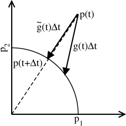
Figure 1: Schematic representation of the momentum components at time $t$ and at time $t+\Delta t$. $g(t)$ is a generic force applied to the system. $\tilde{g}(t)$ is a force which leads to the same change in the kinetic energy as $g(t)$, but minimizes the disturbance.

We now want to design a new correction force $\tilde{g}_{i}(t)$ which gives the same variation of the total energy as Langevin dynamics, thus the same thermalization speed, but minimizes the disturbance on the trajectory. This procedure is exactly the same used by Berendsen et al bere+84jcp , the only difference being that Eq. (4) on the total energy now contains a stochastic term. We first notice that, since the force only acts on the momenta, fixing a value for $H$ is equivalent to fixing a value for $K$. Following Ref. bere+84jcp we quantify the disturbance as $\sum_{i}m_{i}^{-1}(\tilde{g}_{i}(t)dt)^{2}$. As it is seen in Fig. 1, the minimal disturbance for a fixed kinetic energy increment is obtained with a force $\tilde{g}_{i}(t)$ which is proportional to $p_{i}(t)$. Thus $\tilde{g}_{i}(t)=\lambda(t)p_{i}(t)$, where $\lambda(t)$ is chosen so as to enforce a given variation of the total energy. Since $\lambda(t)$ includes a stochastic part, and since the variation of the total energy depends on the momenta only through the kinetic energy $K$, this last relation can be written as

$$\tilde{g}_{i}(t)dt=p_{i}(t)\left[A(K(t))dt+B(K(t))dW(t)\right],$$ (5)

where $A(K)$ and $B(K)$ are arbitrary functions of the kinetic energy. The change in the total energy is then

$$dH=2A(K)Kdt+2B(K)KdW+B^{2}(K)Kdt.$$ (6)

Expressions for $A(K)$ and $B(K)$ can be obtained setting Eq. (4) equal to Eq. (6), resulting in the correction force

$$\tilde{g}_{i}dt=\frac{1}{2\tau}\left[\left(1-\frac{1}{N_{f}}\right)\frac{\bar{K}}{K}-1\right]p_{i}dt\\ +\sqrt{\frac{\bar{K}}{N_{f}K\tau}}p_{i}dW.$$ (7)

This equation is stochastic, with the same noise term used on all the particles. It is also very similar to the expression of the force in the Berendsen algorithm.

The combination of Eqs. (1) and (7) results in a continuous, stochastic dynamics which can be shown to sample exactly the canonical ensemble. The effect of a $\tilde{g}_{i}$ parallel to $p_{i}$ is the same of a rescaling procedure and the enforced increment of the total energy in Eq. (4) is the same as in Ref. buss+07jcp . Thus, Eqs. (1) and (7) represents the continuous version of the velocity rescaling described in Ref. buss+07jcp .

Notably, if $N_{f}=1$, Eq. (7) becomes equivalent to Eq. (2). Thus when the thermostat is applied to a single degree of freedom, it is completely equivalent to a Langevin thermostat. One can perform Langevin molecular dynamics by applying a thermostat per degree of freedom, or stochastic rescaling by applying a single thermostat to the total kinetic energy. Intermediate schemes can be designed, where a thermostat is applied on each molecule or group of atoms.

II Finite timestep algorithm

In the practical implementation, time is incremented in discrete steps, and the Trotter decomposition scheme tuck+92jcp ; buss-parr07pre can be used to separate the integration of Hamilton equations and the update of the momenta due to $\tilde{g}$. The former is then integrated using standard velocity-Verlet, while for the latter we need to integrate Eq. (7). A possible approach is to consider the propagation of kinetic energy when the momenta evolve according to Eq. (7), as it is done in the appendix of Ref. buss+07jcp . The analytical solution of Eq. (7) for a finite time $\Delta t$ is

$$p_{i}(t+\Delta t)=\alpha(t)p_{i}(t),$$ (8a)

where

$$\alpha^{2}(t)=c+\frac{(1-c)(S_{N_{f}-1}(t)+R^{2}(t))\bar{K}}{N_{f}K(t)}\\ +2R(t)\sqrt{\frac{c(1-c)\bar{K}}{N_{f}K(t)}}.$$ (8b)

Here $c=e^{-2\gamma\Delta t}=e^{-\Delta t/\tau}$, $R(t)$ is a Gaussian number with unitary variance and $S_{N_{f}-1}$ is the sum of $N_{f}-1$ independent, squared, Gaussian numbers. Equation (8) has been obtained enforcing the evolution of the kinetic energy, thus, strictly speaking, it does not fix the sign of $\alpha$. A more rigorous analysis shows that the sign of $\alpha$ should be chosen as

$$\text{sign}(\alpha(t))=\text{sign}\left(R(t)+\sqrt{\frac{cN_{f}K(t)}{(1-c)\bar{K}}}\right),$$ (9)

to keep into account the finite probability to observe a flip of the momenta $p_{i}$ when the force in Eq. (7) is applied. The Gaussian number in Eq. (9) needs to be the same that is used in Eq. (8). The probability to observe the flip is extremely small if $N_{f}$ is large and $c\approx 1$, which is the usual case when the thermostat is used as global and $\tau>\Delta t$. This is the case in Ref. buss+07jcp , where we set $\alpha>0$. On the other hand, when the thermostat acts on a few degrees of freedom, the sign of $\alpha$ needs to be calculated by means of Eq. (9). This is always the case for Langevin dynamics. With simple manipulation, it can be shown that for $N_{f}=1$ the integration scheme given by Eqs. (8) and (9), combined with velocity-Verlet, is completely equivalent to the integration scheme for Langevin dynamics introduced in Ref. buss-parr07pre .

III Examples

Up to now we simply established a theoretical relationship between Langevin dynamics and stochastic rescaling. The outcome is that the effect of the two algorithms on the total energy should be equivalent if the friction in the Langevin dynamics and the relaxation time in the stochastic scale are related by $\tau=(2\gamma)^{-1}$. However, the stochastic rescaling is expected to give better dynamical properties, since only the component of the force which changes the total energy is retained. We test here this affirmations on a simple test-case, namely a Lennard-Jones fluid with density $\rho=.8442$ and temperature $\beta^{-1}=0.722$, which is close to the triple point. Throughout this section we use reduced Lennard-Jones units for temperature, distance and time. We simulate a box containing 108 particles, with periodic boundary conditions, and we cut the interaction at distance 2.5. We set the timestep to $\Delta t=0.005$, which leads to a reasonable conservation of the effective energy buss+07jcp ; buss-parr07pre . We then perform runs of $10^{7}$ steps, with both the local scheme (Langevin dynamics) and the global one (stochastic rescaling), using a broad range of values of the thermostat relaxation time $\tau$.

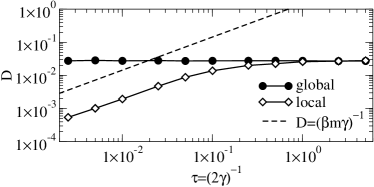
Figure 2: Diffusion coefficient as obtained from thermostated simulations as a function of the thermostat relaxation time $\tau$, for the local and global thermostats as indicated. The statistical error is smaller than the symbol size. As a reference, the diffusion coefficient of a free particle subject to the same Langevin equation is plotted (dashed line). All the quantities are in Lennard-Jones reduced units.

To quantify the disturbance on Hamiltonian dynamics, in Fig. 2 we show the diffusion coefficient as a function of $\tau$, as obtained from the Einstein relations. When the local thermostat is used with a short relaxation time, the diffusion is strongly quenched. This happens when the typical collision time with the external bath $\gamma^{-1}$ is shorter than the typical collision time between the particles, so that the former becomes the real bottleneck for the diffusion process. In the limit of short $\tau$, the equations of motion tend to a high-friction Langevin dynamics. In this case, the observed diffusion coefficient $D$ is proportional to $(\beta m\gamma)^{-1}$, which is the value of the diffusion coefficient for a free particle subject to the same Langevin dynamics. The prefactor is related to the difficulty in crossing the barriers between different liquid configurations. On the contrary, with the global thermostat $D$ is almost independent on $\tau$, indicating that the disturbance on the dynamics is very small and that good estimates of $D$ in the canonical ensemble can be obtained also with a thermostated simulation.

To quantify the equilibration speed we calculate the autocorrelation time of a few global observables. The efficiency of a sampling algorithm is optimal when the autocorrelation time $\tau_{X}$ of the desired quantity $X$ is minimal. If $X$ is the total energy, $\tau_{X}$ also indicates how fast a simulation started from an unlikely configuration is equilibrated. We integrate the autocorrelation function using a windowing function

$$\tau_{X}=\int_{0}^{T}dt\frac{\langle\delta X(0)\delta X(t)\rangle}{\langle\delta X(0)\delta X(0)\rangle}\left(1-\frac{t}{T}\right),$$ (10)

where $\delta X=X-\langle X\rangle$ and $T$ is a large value. The windowing function in parethesis helps the convergence because it weights less the points with larger statistical error. Moreover, Equation (10) is exactly equal to $T\epsilon^{2}(T)/(2\langle\delta X^{2}\rangle)$, where $\epsilon^{2}(T)$ is the mean square error from a time average of length $T$. The relative accuracy in evaluation of $\tau_{X}$ is approximately $\sqrt{2T/T^{\prime}}$, where $T^{\prime}=5\times 10^{4}$ is the total run length. In the following we choose $T=50$, and we expect a relative accuracy on $\tau_{X}$ on the order of 5%. Since $T\gg\tau_{X}$, $\tau_{X}$ is also a good approximation for the autocorrelation time.

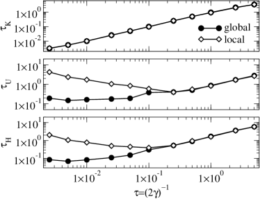
Figure 3: Autocorrelation time of the kinetic ($\tau_{K}$), potential ($\tau_{U}$), and total ($\tau_{H}$) energy, as a function of the thermostat relaxation time $\tau$, for the local and global thermostats as indicated. The statistical error is smaller than the symbol size. All the quantities are in Lennard-Jones reduced units.

In Figure 3 we plot the autocorrelation time of the kinetic energy $\tau_{K}$, of the potential energy $\tau_{U}$ and of the total energy $\tau_{H}$, as a function of the thermostat relaxation time $\tau$. The autocorrelation time of the kinetic energy is completely dictated by the thermostat relaxation time, and independent on the choice of a local or a global scheme. On the contrary, the autocorrelation time of the total energy and of the potential energies are proportional to $\tau$ only in the limit of large $\tau$. In the local scheme, when $\tau$ is smaller than 0.2 the disturbance of the trajectory becomes so large that the phase-space exploration turns out to be slower. Comparing Figs. 2 and 3, it is seen that the optimal value for $\tau$ is the smallest one that still does not affect the diffusion coefficient. When the global scheme is adopted, even small values of $\tau$ can be safely used, resulting in a faster decorrelation of the total energy.

IV Conclusions

In conclusion, we have presented an alternative derivation of the global thermostat introduced in Ref. buss+07jcp . This derivation allows to write continuous equations of motion and shows the analogy between this scheme and the standard Langevin thermostat. Namely, the new scheme can be considered as a global version of the Langevin thermostat, that minimizes the disturbance of the original Hamiltonian dynamics. Finally, we have discussed these properties on a simple test case, showing that the global scheme preserves the dynamical properties. Moreover, using as a measure the autocorrelation time of the total energy, we have shown that the global scheme allows for a faster sampling.

References

- (1) S. Nosé, J. Chem. Phys. 81, 511 (1984).
- (2) W. G. Hoover, Phys. Rev. A 31, 1695 (1985).
- (3) G. J. Martyna, M. L. Klein, and M. Tuckerman, J. Chem. Phys. 97, 2635 (1992).
- (4) D. J. Tobias, G. J. Martyna, and M. L. Klein, J. Phys. Chem. 97, 12959 (1993).
- (5) H. J. C. Berendsen, J. P. M. Postma, W. F. van Gunsteren, A. DiNola, and J. R. Haak, J. Chem. Phys. 81, 3684 (1984).
- (6) T. Schneider and E. Stoll, Phys. Rev. B 17, 1302 (1978).
- (7) G. Bussi, D. Donadio, and M. Parrinello, J. Chem. Phys. 126, 014101 (2007).
- (8) D. Donadio and G. Galli, Phys. Rev. Lett. 99, 255502 (2007).
- (9) F. Bruneval, D. Donadio, and M. Parrinello, J. Phys. Chem. B 111, 12219 (2007).
- (10) A. Barducci, G. Bussi, and M. Parrinello, Phys. Rev. Lett. 100, 020603 (2008).
- (11) T. Zykova, G. Bussi, and M. Parrinello, In preparation.
- (12) C. W. Gardiner, Handbook of Stochastic Methods, Springer, Berlin, third edition, 2003.
- (13) M. Tuckerman, B. J. Berne, and G. J. Martyna, J. Chem. Phys. 97, 1990 (1992).
- (14) G. Bussi and M. Parrinello, Phys. Rev. E 75, 056707 (2007).