Real Roots of Random Polynomials and Zero Crossing Properties of Diffusion Equation.

Abstract

We study various statistical properties of real roots of three different classes of random polynomials which recently attracted a vivid interest in the context of probability theory and quantum chaos. We first focus on gap probabilities on the real axis, i.e. the probability that these polynomials have no real root in a given interval. For generalized Kac polynomials, indexed by an integer $d$, of large degree $n$, one finds that the probability of no real root in the interval $[0,1]$ decays as a power law $n^{-\theta(d)}$ where $\theta(d)>0$ is the persistence exponent of the diffusion equation with random initial conditions in spatial dimension $d$. For $n\gg 1$ even, the probability that they have no real root on the full real axis decays like $n^{-2(\theta(2)+\theta(d))}$. For Weyl polynomials and Binomial polynomials, this probability decays respectively like $\exp{(-2\theta_{\infty}}\sqrt{n})$ and $\exp{(-\pi\theta_{\infty}\sqrt{n})}$ where $\theta_{\infty}$ is such that $\theta(d)=2^{-3/2}\theta_{\infty}\sqrt{d}$ in large dimension $d$. We also show that the probability that such polynomials have exactly $k$ roots on a given interval $[a,b]$ has a scaling form given by $\exp{(-N_{ab}\,\tilde{\varphi}(k/N_{ab}))}$ where $N_{ab}$ is the mean number of real roots in $[a,b]$ and $\tilde{\varphi}(x)$ a universal scaling function. We develop a simple Mean Field (MF) theory reproducing qualitatively these scaling behaviors, and improve systematically this MF approach using the method of persistence with partial survival, which in some cases yields exact results. Finally, we show that the probability density function of the largest absolute value of the real roots has a universal algebraic tail with exponent ${-2}$. These analytical results are confirmed by detailed numerical computations. Some of these results were announced in a recent letter [G. Schehr and S. N. Majumdar, Phys. Rev. Lett. 99, 060603 (2007)].

I Introduction

Despite several decades of research, understanding the zero crossing properties of non-Markov stochastic processes remains a challenging issue. Among them, the persistence probability $p_{0}(t)$ received a particular attention, especially in the context of many-body non-equilibrium statistical physics, both analytically satya_review as well as experimentally marcos ; persist_exp_froth ; persist_exp_steps ; persist_diffusion_exp . The persistence $p_{0}(t)$ for a time dependent stochastic process with zero mean is defined as the probability that it has not changed sign up to time $t$. In various physical situations, $p_{0}(t)$ has a power law tail $p_{0}(t)\sim t^{-\theta}$ where $\theta$ turns out to be a non-trivial exponent whenever the stochastic process under study has a non Markovian dynamics. One such example is the diffusion, or heat equation in space dimension $d$ where a scalar field $\phi({\mathbf{x}},t)$ evolves according to the deterministic equation

$$\partial_{t}\phi({\mathbf{x}},t)=\nabla^{2}\phi({\mathbf{x}},t)\,,$$ (1)

with random initial conditions $\phi({\mathbf{x}},t=0)=\psi({\mathbf{x}})$ where $\psi({\mathbf{x}})$ is a Gaussian random field of zero mean with delta correlations $[\psi({\mathbf{x}})\psi({\mathbf{x}^{\prime}})]_{\rm ini}=\delta^{d}({\mathbf{x}}-{\mathbf{x}^{\prime}})$. We use the notation $[...]_{\rm ini}$ to denote an average over the initial condition. For a system of linear size $L$, the persistence $p_{0}(t,L)$ is the probability that $\phi({\mathbf{x}},t)$, at some fixed point ${\mathbf{x}}$ in space, does not change sign up to time $t$. The initial condition being (statistically) invariant under translation in space, this probability does not depend on the position ${\mathbf{x}}$. In the scaling limit $t\gg 1$, $L\gg 1$ keeping the ratio $t/L^{2}$ fixed, it was found in Ref. persist_diffusion that $p_{0}(t,L)$ takes the scaling form

$$p_{0}(t,L)\propto L^{-2\theta(d)}h(L^{2}/t)\;,$$ (2)

where $h(u)\sim c^{\rm st}$, a constant independent of $L$ and $t$, for $u\ll 1$ and $h(u)\propto u^{\theta(d)}$ for $u\gg 1$ where $\theta(d)$ is a $d$-dependent exponent. This implies that in the $L\to\infty$ limit, $p_{0}(t)\equiv p_{0}(t,L\to\infty)\sim t^{-\theta(d)}$ for large $t$. It was shown in Ref. persist_diffusion that the probability ${\cal P}_{0}(T)$ that a Gaussian stationary process (GSP) with zero mean and correlations $[\cosh(T/2)]^{-d/2}$ decays for large $T$ as ${\cal P}_{0}(T)\sim\exp{[-\theta(d)T]}$ where $\theta(d)$ is the same as the persistence exponent in diffusion equation. This exponent $\theta(d)$ was measured in numerical simulations persist_diffusion ; newman_diffusion , yielding for instance $\theta_{\rm sim}(1)=0.12050(5)$, $\theta_{\rm sim}(2)=0.1875(1)$. The case of dimension $d=1$ is particularly interesting because $\theta(1)$ was determined experimentally using NMR techniques to measure the magnetization of spin polarized Xe gas persist_diffusion_exp , yielding $\theta_{\rm exp}(1)=0.12$ in good agreement with numerical simulations. In the limit of large dimension $d$, which will be of interest in the following, one can show that $\theta(d)=2^{-3/2}\theta_{\infty}\sqrt{d}$ where $\theta_{\infty}$ is the decay constant associated with the no zero crossing probability of the GSP with Gaussian correlations $\exp{(-T^{2}/2)}$, which was studied in the past by engineers, in particular in the context of fading of long-wave radio signals (see for instance Ref. palmer ).

A seemingly unrelated topic concerns the study of random algebraic equations which, since the first work by Bloch and Pólya bloch in the 30’s, has now a long story bharucha ; farahmand . Recently it has attracted a renewed interest in the context of probability and number theory edelman as well as in the field of quantum chaos bogomolny . In a recent letter us_prl , we have established a close connection between zero crossing properties of the diffusion equation with random initial conditions (1) and the real roots of real random polynomials (i.e. polynomials with real random coefficients). In Ref. us_prl , we focused on a class of real random polynomials $K_{n}(x)$ of degree $n$, the so called generalized Kac polynomials, indexed by an integer $d$

$$K_{n}(x)=a_{0}+\sum_{i=1}^{n}a_{i}\;i^{\tfrac{d-2}{4}}x^{i}\;.$$ (3)

Here, and in the following, $a_{i}$’s are independent real Gaussian random variables of zero mean and unit variance $\langle a_{i}a_{j}\rangle=\delta_{ij}$ where we use the notation $\langle...\rangle$ to denote an average over the random coefficients $a_{i}$. In the case of $d=2$, these polynomials reduce to the standard Kac polynomials kac_1 , which have been extensively studied in the past (see for instance Ref. edelman for a recent review). In that case, we will see below that the statistics of real roots of $K_{n}(x)$ is identical in the $4$ sub-intervals $[-\infty,-1],[-1,0],[0,1]$ and $[1,+\infty]$. Instead, for $d\neq 2$, which was studied in Ref. das , the statistical behavior of real roots of $K_{n}(x)$ depend on $d$ in the inner intervals, while it is identical to the case $d=2$ in the outer ones. Focusing on the interval $[0,1]$, we asked the question : what is the probability $P_{0}([0,x],n)$, $0<x<1$, that $K_{n}(x)$ has no real root in the interval $[0,x]$ ? Such probabilities were often studied in the context of random matrices, where they are known as gap probabilities mehta and in a recent work dembo , Dembo et al. showed that, for random polynomials $K_{n}(x)$ with $d=2$, $P_{0}([0,1],n)\propto n^{-\zeta(2)}$ where the exponent $\zeta(2)=0.190(8)$ was computed numerically. In Ref. us_prl , by mapping these two random processes (1) and (3) onto the same GSP, we showed that in the limit $1-x\ll 1\ll n$ keeping $n(1-x)$ fixed, one has (similarly to Eq. (2))

$$P_{0}([0,x],n)\propto n^{-\theta(d)}h^{-}(n(1-x))\;,$$ (4)

with $h^{-}(y)\to 1$ for $y\ll 1$ and $h^{-}(y)\sim y^{\theta(d)}$ for $y\gg 1$, yielding in particular $P_{0}([0,1],n)\propto n^{-\zeta(d)}$ thus identifying $\zeta(d)=\theta(d)$. We then extended our study to the probability $P_{k}([0,1],n)$ that generalized Kac polynomials have exactly $k$ real roots in $[0,1]$ and we showed that it has an unusual scaling form (for large $k$, large $n$, but keeping the ratio $k/\log n$ fixed)

$$P_{k}([0,1],n)\propto n^{-\tilde{\varphi}\left(\tfrac{k}{\log n}\right)}\;,$$ (5)

where $\tilde{\varphi}(y)$ is a large deviation function, with $\tilde{\varphi}(0)=\theta(d)$. In both cases, our numerical analysis suggested that $h^{-}(y)$ and $\tilde{\varphi}(y)$ are universal in the sense that they are independent of the distribution of $a_{i}$ provided $\langle a_{i}^{2}\rangle$ is finite. The purpose of the present paper is twofold : (i) we will give detailed derivations of the results announced in Ref. us_prl together with some new results, like the distribution of the largest real root, for generalized Kac polynomials $K_{n}(x)$ (3), (ii) we extend these results (4, 5) to two other classes of random polynomials which were recently considered in the literature. First we will study Weyl polynomials $W_{n}(x)$ defined as

$$W_{n}(x)=\sum_{i=0}^{n}a_{i}\;\frac{x^{i}}{\sqrt{i!}}\;.$$ (6)

Recently, the distribution of complex zeros of Weyl polynomials with complex coefficients were observed experimentally in a degenerate rotating quasi-ideal atomic Bose gas castin_complex_exp . Here we will focus instead on the real roots of such polynomials (6) with real coefficients. Besides, we will consider binomial polynomials $B_{n}(x)$ defined as

$$B_{n}(x)=\sum_{i=0}^{n}a_{i}\;\sqrt{n\choose i}x^{i}\;.$$ (7)

As is pointed out by Edelman and Kostlan edelman , ”this particular random polynomial is probably the more natural definition of a random polynomial”. In the literature, they are sometimes called $SO(2)$ random polynomials because their $m$-point joint probability distribution of zeros is $SO(2)$ invariant for all $m$ bleher . We will show below that the gap probabilities for these classes of random polynomials (6, 7) are closely related to the persistence probability for the diffusion equation in the limit of large dimension. Our main results, together with the layout of the paper, are summarized below.

1. In section II, we briefly recall the main properties of the persistence probability, $p_{0}(t,L)$, for the diffusion equation with random initial conditions. In section II-A, we recall the finite size scaling for $p_{0}(t,L)$ in dimension $d$ whereas in section II-B, we focus on the limit $d\to\infty$.

2. Section III is devoted to real random polynomials, where our main results are presented. In section III-A, we present a detailed study of the density of real roots for these three classes of polynomials, which turns out to behave quite differently in all the the three cases under investigations (3, 6, 7) . In section III-B, we will turn to the analysis of gap probabilities, which we will first analyse from the point of view of two-point correlations. Next, we will present a mean field approach, or Poissonian approximation, which neglects the correlations between the real roots of these polynomials, to compute the gap probabilities. We will further show how this mean field approximation can be systematically improved using the persistence probability with partial survival satya_partial , which in some cases even yields exact results. In particular we show that the probability $q_{0}(n)$ that these polynomials have no root on the full real axis is given by

   $$q_{0}(n)\sim n^{-2(\theta(d)+\theta(2))}\hskip 44.10185pt{\rm for\;}K_{n}(x)\;,$$

   $$q_{0}(n)\sim\exp{(-2\theta_{\infty}}\sqrt{n})\hskip 36.98866pt{\rm for\;}W_{n}(x)\;,$$

   $$q_{0}(n)\sim\exp{(-\pi\theta_{\infty}\sqrt{n})}\hskip 35.85031pt{\rm for\;}B_{n}(x)\;.$$ (8)

   In section III-C, we will then generalize this study to the probability that these polynomials have exactly $k$ real roots on a given real interval. Extending the results obtained in Ref. us_prl for $K_{n}(x)$ like in Eq. (5), to Weyl and Binomial polynomials, we will show that the probability $q_{k}(n)$ that $W_{n}(x)$ and $B_{n}(x)$ have exactly $k$ roots on the full real axis has a scaling form (for large $k$, large $n$, but keeping the ratio $k/\sqrt{n}$ fixed) given by

   $$q_{k}(n)\sim\exp{[-\sqrt{n}\tilde{\varphi}\left({k}/{\sqrt{n}}\right)]}\;,$$ (9)

   where $\tilde{\varphi}(y)$ is a large deviation function, which depends on the polynomials under consideration $W_{n}(x)$ or $B_{n}(x)$. We will also show that these scaling forms in Eq. (5, 9) can be qualitatively described by the aforementioned mean field approximation. To end up, we study in section III-D the probability density (p.d.f.) $p_{\rm max}(x)$ of the largest absolute value of the real roots and obtain the exact asymptotic result

   $$p_{\rm max}(x)\propto\frac{1}{x^{2}}\;,\;x\gg 1\;,$$ (10)

   for all the three classes of random polynomials under investigation. All our analytical results will be verified by numerical computations and some details of the analytical computations involved in this section have been left in Appendices A,B, C, D and E.

3. Finally section IV contains our conclusions and perspectives.

II A brief overview on persistence for diffusion equation in dimension $d$

II.1 Persistence exponent $\theta(d)$ and finite size scaling

We consider a scalar field $\phi({\mathbf{x}},t)$ in a $d$-dimensional space which evolves in time under the diffusion equation (1). For a system of linear size $L$, the solution of the diffusion equation in the bulk of the system is

$$\phi({\mathbf{x}},t)=\int_{|{\mathbf{y}}|\leq L}d{\mathbf{y}}\;{\cal G}({\mathbf{x}}-{\mathbf{y}},t)\;\psi({\mathbf{y}})\quad,\quad{\cal G}({\mathbf{x}})=(4\pi t)^{-d/2}\exp{(-{\mathbf{x}}^{2}/4t)}\,,$$ (11)

where $\psi(\mathbf{x})=\phi(\mathbf{x},0)$ is the initial uncorrelated Gaussian field. Since Eq. (11) is linear, $\phi({\mathbf{x}},t)$ is a Gaussian variable for all time $t\geq 0$. Therefore its zero crossing properties are completely determined by the two time correlator $[\phi({\mathbf{x}},t)\phi({\mathbf{x}},t^{\prime})]_{\rm ini}$. To study the persistence probability $p_{0}(t,L)$ it is customary to study the normalized process $X(t)=\phi({\mathbf{x}},t)/[\phi({\mathbf{x}},t)^{2}]_{\rm ini}^{1/2}$ satya_review . Its autocorrelation function $a(t,t^{\prime})=[X(t)X(t^{\prime})]_{\rm ini}$ is computed straightforwardly from the solution in Eq. (11). One obtains $a(t,t^{\prime})\equiv a(\tilde{t},\tilde{t}^{\prime})$ with $\tilde{t}=t/L^{2}$, $\tilde{t}^{\prime}=t^{\prime}/L^{2}$ and

$$a(\tilde{t},\tilde{t}^{\prime})=\begin{cases}\left(\frac{4\tilde{t}\tilde{t}^{\prime}}{(\tilde{t}+\tilde{t}^{\prime})^{2}}\right)^{d/4}\quad,\quad\tilde{t},\tilde{t}^{\prime}\ll 1\\ 1\quad,\quad\tilde{t},\tilde{t}^{\prime}\gg 1\,.\end{cases}$$ (12)

We first focus on the time regime $\tilde{t},\tilde{t}^{\prime}\ll 1$. In terms of logarithmic time variable $T=\log\tilde{t}$, $X(T)$ is a GSP with correlator

$$a(T,T^{\prime})\equiv a(T-T^{\prime})=[{\rm cosh}(|T-T^{\prime}|/2)]^{-d/2}\;,$$ (13)

which decays exponentially for large $|T-T^{\prime}|$. Thus the persistence probability $p_{0}(t,L)$, for $t\ll L^{2}$, reduces to the computation of the probability ${\cal P}_{0}(T)$ of no zero crossing of $X(T)$ in the interval $[0,T]$. It is well known slepian that if $a(T)<1/T$ at large $T$ then ${\cal P}_{0}(T)\sim\exp[-\theta T]$ for large $T$ where the decay constant $\theta$ depends on the full stationary correlator $a(T)$. Reverting back to the original time $\tilde{t}=e^{T}$, one finds $p_{0}(t,L)\sim t^{-\theta(d)}$, for $t\ll L^{2}$. In the opposite limit $t\gg L^{2}$, one has $p_{0}(t,L)\to A_{L}$, a constant which depends on $L$. These two limiting behaviors of $p_{0}(t,L)$ can be combined into a single finite size scaling form as in Eq. (2).

Despite many efforts, there exists no exact result for $\theta(d)$. However various approximation methods have been developed to estimate it. One of the most powerful is the so called Independent Interval Approximation (IIA) IIA , which assumes the statistical independence of the intervals between successive zeros of $\phi(\mathbf{x},t)$. This gives e.g. $\theta_{\rm IIA}(1)~{}=~{}0.1203...$, $\theta_{\rm IIA}(2)~{}=~{}0.1862...$ persist_diffusion in remarkable agreement with numerical simulations. A more systematic approach is via persistence with partial survival satya_partial , which we will use below (see section III-B). An alternative systematic approach consists in performing a small $d$ expansion hilhorst yielding $\theta(d)=d/4-0.12065...d^{3/2}+...$, which would certainly require higher order terms to make it numerically competitive. Yet another systematic approach is a series expansion introduced in the context of ”discrete time persistence”, yielding results for $\theta(d)$ which are in very good agreement with numerical simulations ehrhardt .

II.2 Persistence in the limit of large dimension $d$

As we will see later, some statistical properties of the real roots of the polynomials $W_{n}(x)$ (6) and $B_{n}(x)$ (7) turn out to be related to the statistics of zero crossings of the diffusion equation in the limit of large dimension $d$. To study the persistence probability in that limit one performs a rescaling of the $T$ variable in Eq. (13), $T=2^{3/2}\tilde{T}/\sqrt{d}$ such that

$$a(T-T^{\prime})=a\left(2^{3/2}\frac{\tilde{T}-\tilde{T}^{\prime}}{\sqrt{d}}\right)\sim\exp{\left[-\frac{1}{2}(\tilde{T}-\tilde{T}^{\prime})^{2}\right]}\;,\;d\gg 1\,.$$ (14)

Therefore in the limit of large dimension $d$, one has $\theta(d)=2^{-3/2}\theta_{\infty}\sqrt{d}$ where $\theta_{\infty}$ is the decay constant associated with the no zero crossing probability of the GSP with correlator $\exp{[-\frac{1}{2}(T-T^{\prime})^{2}]}$. Even in that limit, there is no exact result for $\theta_{\infty}$. However, it can be approximately estimated using IIA IIA , yielding $\theta_{\infty,{\rm IIA}}=0.411497...$ persist_diffusion in very good agreement with numerical simulations $\theta_{\infty,{\rm sim}}=0.417(3)$ newman_diffusion .

III Random polynomials

We now focus on statistical properties of the real roots of random polynomials, extending our previous study presented in Ref. us_prl . Being Gaussian processes, the statistical properties of these polynomials are determined by the $2$-point correlators $C_{n}(x,y)$, given by

$$C_{n}(x,y) = \langle K_{n}(x)K_{n}(y)\rangle=1+\sum_{i=1}^{n}i^{\tfrac{d-2}{2}}\;(xy)^{i}\;\hskip 85.35826pt{\rm for\;Kac\;polynomials}\;,$$ (15)

$$C_{n}(x,y) = \langle W_{n}(x)W_{n}(y)\rangle=\sum_{i=0}^{n}\frac{(xy)^{i}}{i!}\;\hskip 120.92421pt{\rm for\;Weyl\;polynomials}\;,$$ (16)

$$C_{n}(x,y) = \langle B_{n}(x)B_{n}(y)\rangle=\sum_{i=0}^{n}{n\choose i}(xy)^{i}=(1+xy)^{n}\;\hskip 51.21504pt{\rm for\;Binomial\;polynomials}\;.$$ (17)

For simplicity, we chose the same notation $C_{n}(x,y)$ for the three classes of polynomials under study, and we will do so for other quantities. In the following, these three polynomials will be treated separately so this should not induce any confusion. For later purposes it is convenient to introduce the normalized correlator $\hat{C}_{n}(x,y)$ with

$$\hat{C}_{n}(x,y)=\frac{C_{n}(x,y)}{\sqrt{C_{n}(x,x)C_{n}(y,y)}}\;.$$ (18)

Notice that $\hat{C}_{n}(x,y)=\hat{C}_{n}(1/x,1/y)$ for Kac polynomials $K_{n}(x)$ with $d=2$ and for Binomial polynomials $B_{n}(x)$.

III.1 Density and mean number of real roots

Let us denote $\lambda_{1},\lambda_{2},...,\lambda_{p}$ the $p$ real roots (if any) of one of these random polynomials in Eq. (3, 6, 7). The mean density of real roots $\rho_{n}(x)$ is given by

$$\rho_{n}(x)=\sum_{i=1}^{p}\langle\delta(x-\lambda_{i})\rangle=\langle|K_{n}^{\prime}(x)|\delta(K_{n}(x))\rangle\;,\hskip 28.45274pt{\rm for\;Kac\;polynomials}\;,$$ (19)

and similarly for Weyl polynomials $W_{n}(x)$ and Binomial polynomials $B_{n}(x)$. Under this form (19), one observes that the computation of the mean density involves the joint distribution of the polynomial $K_{n}(x)$ and its derivative $K^{\prime}_{n}(x)$ which is simply a bivariate Gaussian distribution. Thus computing $\rho_{n}(x)$ involves a double integration of a bivariate Gaussian distribution. This can be easily performed to obtain the following well known result

$$\rho_{n}(x)=\frac{\sqrt{c_{n}(x)(c_{n}^{\prime}(x)/x+c_{n}^{\prime\prime}(x))-[c_{n}^{\prime}(x)]^{2}}}{2\pi c_{n}(x)}\;,\;c_{n}(x)=C_{n}(x,x)\;.$$ (20)

This formula (20) can be written in a very compact way edelman :

$$\rho_{n}(x)=\frac{1}{\pi}\sqrt{\partial_{u}\partial_{v}\log C_{n}(u,v)}\bigg{|}_{u=v=x}\;.$$ (21)

For these different polynomials in Eq. (3, 6, 7), we will be interested in the number of real roots on a given interval $[a,b]$, which we will denote $N_{n}[a,b]$. Being a random variable, we will focus on its moments $\langle N^{k}_{n}[a,b]\rangle$, with $k\in\mathbb{N}$. In particular, one has from the definition of $\rho_{n}(x)$ in Eq. (19)

$$\langle N_{n}[a,b]\rangle=\int_{a}^{b}\rho_{n}(x)\,dx\;,$$ (22)

and higher cumulants will be considered below.

III.1.1 Generalized Kac polynomials

One remarkable property of the generalized Kac polynomials $K_{n}(x)$ is that, in the large $n$ limit, the roots in the complex plane tend to accumulate close to the unit circle centered at the origin.

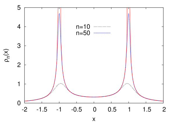
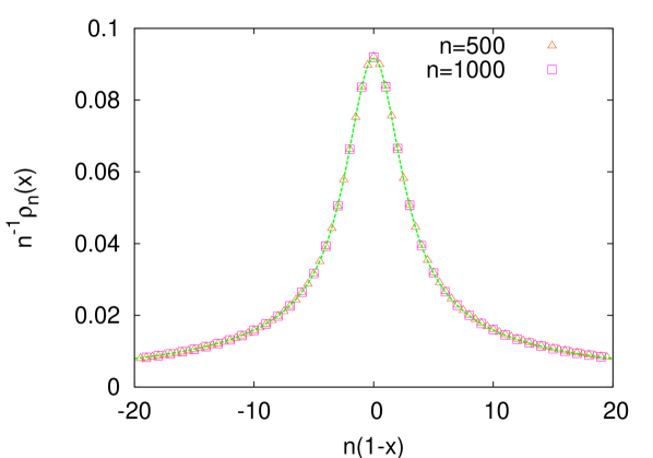
Figure 1: Left : Mean density of real roots $\rho_{n}(x)$ for Kac polynomials $K_{n}(x)$ (3) and $d=2$ as a function of $x$ for different values of $n=10,50$ (dotted lines). The solid line is the analytic expression $\rho_{\infty}(x)$ in Eq. (25) for $|x|<1$ and in Eq. (27) for $|x|>1$. Right : Plot of $n^{-1}\rho_{n}(x)$ as a function of $n(1-x)$ for $n=500,1000$ (and thus $x$ close to $\pm 1$). The dotted line is the function $\rho^{K}(y)$ in Eq. (31). There is no fitting parameter.

In the left panel of Fig. 1, we show a plot of the density of real roots $\rho_{n}(x)$ for $d=2$ computed from Eq. (21) for different values of $n=10$ and $50$. In the large $n$ limit, one clearly sees that the real roots of such polynomials are concentrated around $x=\pm 1$, where the density is diverging. This can be seen by computing $\rho_{n}(\pm 1)$ from Eq. (21)

$$\rho_{n}(\pm 1)=\frac{1}{\pi}\frac{\left((1+{\cal H}(n,1-d/2)){\cal H}(n,-d/2-1)-{\cal H}(n,-d/2)^{2}\right)^{\tfrac{1}{2}}}{1+{\cal H}(n,1-d/2)}\propto\frac{2n}{\pi(d+2)}\sqrt{\frac{d}{d+4}}\;,$$ (23)

where ${\cal H}(n,r)=\sum_{k=1}^{n}k^{-r}$ is a generalized harmonic number grad . To obtain the asymptotic behavior in the large $n$ limit of the above equation (23) we used ${\cal H}(n,r)\propto n^{1-r}/(1-r)$, for large $n$ and $r<1$.

Away from these singularities, $\rho_{n}(x)$ has a good limit when $n\to\infty$. However, one has to treat separately the cases $|x|<1$ and $|x|>1$. For $|x|<1$, the calculation is straightforward because $C_{n}(x,y)$ in Eq. (15) has a good limit $n\to\infty$ when $x,y<1$. This yields

$$\rho_{\infty}(x)=\frac{\left[{{\rm Li}_{-1-d/2}(x^{2})(1+{\rm Li}_{1-d/2}(x^{2}))-{\rm Li}^{2}_{-d/2}(x^{2})}\right]^{\tfrac{1}{2}}}{\pi|x|(1+{\rm Li}_{1-d/2}(x^{2}))}\quad,\quad|x|<1\;,$$ (24)

where ${\rm Li}_{n}(z)=\sum_{i=1}^{\infty}z^{i}/i^{n}$ is the polylogarithm function grad . In particular, one has $\rho_{\infty}(0)=1/\pi$ for all $d$, and $\rho_{\infty}(x)\sim(d/2)^{\tfrac{1}{2}}(2\pi((1-x)))^{-1}$ for $x\to 1^{-}$. For instance, one has for $|x|<1$

$$\rho_{\infty}(x)=\frac{1}{\pi(1-x^{2})}\quad{\rm in}\quad d=2\quad,\quad\rho_{\infty}(x)=\frac{1}{\pi(1-x^{2})}\sqrt{\frac{x^{8}+2x^{6}-4x^{4}+2x^{2}+1}{x^{8}-2x^{6}+3x^{4}-2x^{2}+1}}\quad{\rm in}\quad d=4\;.$$ (25)

For $|x|>1$, the analysis is different because the correlator $C_{n}(x,y)$ in Eq. (15) does not converge any more in the limit $n\to\infty$ when $x,y>1$. Instead, one has in that case (see also Ref. das )

$$C_{n}(x,y)=1+\sum_{i=1}^{n}i^{\tfrac{d-2}{2}}\;(xy)^{i}\propto\frac{n^{\tfrac{d-2}{2}}(xy)^{n+1}}{xy-1}\;,\;x,y>1\;.$$ (26)

This leads to the expression for the density $\rho_{\infty}(x)$ for $|x|>1$ :

$$\rho_{\infty}(x)=\frac{1}{\pi(x^{2}-1)}\;,$$ (27)

independently of $d$. To understand better the divergence of $\rho_{n}(x)$ around $x=\pm 1$ (23) when $n\gg 1$, we focus on $\rho_{n}(x)$ around $x=1$. In the limit $n\gg 1$ and $1-x\ll 1$ keeping $y=n(1-x)$ fixed, one shows in Appendix A (see also fyodorov ) that

$$\rho_{n}(x)=n\rho^{K}(n(1-x))\;,\;\rho^{K}(y)=\frac{1}{\pi}\sqrt{\frac{I_{d/2+1}(y)}{I_{d/2-1}(y)}-\left(\frac{I_{d/2}(y)}{I_{d/2-1}(y)}\right)^{2}}\;,$$ (28)

$$I_{m}(y)=\int_{0}^{1}dx\;x^{m}\exp{(-2yx)}\;.$$ (29)

One has $\rho^{K}(0)=\frac{2}{\pi}\frac{1}{d+2}\sqrt{\frac{d}{d+4}}$, recovering the large $n$ behavior in Eq. (23) and its asymptotic behaviors are given by (see Appendix A)

$$\rho^{K}(y)\sim\begin{cases}\frac{1}{2\pi y}\sqrt{\frac{d}{2}}\quad,\quad y\to+\infty\\ \frac{1}{2\pi|y|}\quad,\quad y\to-\infty\;.\end{cases}$$ (30)

For instance, one has

$$\rho^{K}(y)=\frac{1}{2\pi}\left(\frac{1}{y^{2}}-\frac{1}{\sinh^{2}{y}}\right)^{1/2}\quad,\quad{\rm{in}}\quad d=2\;.$$ (31)

In the right panel of Fig. 1, we show a plot of $n^{-1}\rho_{n}(x)$, where $\rho_{n}(x)$ is given in Eq. (116), as a function of $n(1-x)$ for $d=2$ and different large values of $n=500,1000$ together with the asymptotic results in Eq. (31) : we find a very good agreement with these analytic predictions (28, 31).

Having computed the mean density of real roots, we now focus on $\langle N_{n}([a,b])\rangle$. On the interval $[0,1]$ the main contribution to the mean number of real roots comes, for large $n$, from the vicinity of $x=1$. Therefore, to compute $\langle N_{n}[0,1]\rangle$ to leading order in $n$, one uses the scaling form for the density in Eq. (28), valid close to $x=1$, and the asymptotic behavior in Eq. (30) to obtain for $n\gg 1$

$$\langle N_{n}[0,1]\rangle=\langle N_{n}[-1,0]\rangle=\int_{0}^{n}\rho^{K}(y)dy+{\cal O}(1)=\frac{1}{2\pi}\sqrt{\frac{d}{2}}\log{n}+{\cal O}(1)\;,$$ (32)

where the corrections of order ${\cal O}(1)$ receive contributions from the whole interval $[0,1]$ (not only from the vicinity of $x=\pm 1$).

Similarly, one gets from Eq. (28) and Eq. (30):

$$\langle N_{n}[-\infty,-1]\rangle=\langle N_{n}[1,+\infty]\rangle=\int_{0}^{n}\rho^{K}(-y)dy+{\cal O}(1)=\frac{1}{2\pi}\log{n}+{\cal O}(1)\;,$$ (33)

which is independent of $d$ das . From Eqs (32, 33) we compute the total number of roots on the real axis :

$$\langle N_{n}([-\infty,+\infty])\rangle=\frac{1}{\pi}\left(1+\sqrt{\frac{d}{2}}\right)\log{n}+{\cal O}(1)\;,$$ (34)

thus recovering, in a way similar to the one used in Ref. edelman for $d=2$, the result of das . Notice that for $d=2$ the higher order terms of the large $n$ expansion in this formula (34) have been obtained by various authors (see for instance Ref. edelman ; wilkins ), although, to our knowledge, they have not been computed for $d\neq 2$.

In view of future purposes, we also compute $\langle N_{n}[0,x]\rangle$ in the asymptotic limit where $n\gg 1$, and $0<1-x\ll 1$ with $n(1-x)$ kept fixed :

$$\langle N_{n}[0,x]\rangle=\langle N_{n}[0,1]\rangle-\eta_{-}(n(1-x))\;,$$ (35)

$$\eta_{-}(y)=\int_{0}^{y}du\;\rho^{K}(u)\;,$$ (36)

such that $\eta_{-}(0)=0$ and with the asymptotic behavior obtained from Eq. (30)

$$\eta_{-}(y)\sim\frac{1}{2\pi}\sqrt{\frac{d}{2}}\log{y}\quad,\quad y\to\infty\;.$$ (37)

Similarly, we compute $\langle N_{n}[x,\infty]\rangle$ when $x>1$ and obtain for $n\gg 1$ and $0<x-1\ll 1$ keeping $y=n(x-1)$ fixed

$$\langle N_{n}[x,\infty]\rangle=\langle N_{n}[1,\infty]\rangle-\eta_{+}(n(x-1))\;,$$ (38)

$$\eta_{+}(y)=\int_{0}^{y}du\rho^{K}(-u)\;,$$ (39)

such that $\eta_{+}(0)=0$ and with the asymptotic behavior obtained from Eq. (30)

$$\eta_{+}(y)\sim\frac{1}{2\pi}\log{y}\quad,\quad y\to\infty\;.$$ (40)

We conclude this subsection by noting that, for $d=2$, the statistics of real roots of $K_{n}(x)$ is identical in the $4$ sub-intervals $[-\infty,-1],[-1,0],[0,1]$ and $[1,+\infty]$. Instead, for $d\neq 2$, the statistical behavior of real roots of $K_{n}(x)$ depend on $d$ in the two inner intervals, while it is identical to the case $d=2$ in the two outer ones. In addition, we will see below that the polynomials $K_{n}(x)$ (3) take independent values in these 4 subintervals.

III.1.2 Weyl polynomials

For Weyl polynomials $W_{n}(x)$ in Eq. (6), the expression of the correlation function (16) together with the expression for the density in Eq. (21) yields

$$\rho_{n}(x)=\frac{1}{\pi}\sqrt{1+\frac{x^{2n}(x^{2}-n-1)}{e^{x^{2}}\Gamma(n+1,x^{2})}-\frac{x^{4n+2}}{[e^{x^{2}}\Gamma(n+1,x^{2})]^{2}}}\;,$$ (41)

where $\Gamma(n,x)=\int_{x}^{\infty}dte^{-t}t^{n-1}$ is the incomplete gamma function grad . In Fig. 2, we show a plot of $\rho_{n}(x)$ (41) for different values of $n=50,100$ and $500$. One obtains straightforwardly, in the limit $n\to\infty$ the uniform density

$$\rho_{\infty}(x)=\frac{1}{\pi}\;.$$ (42)

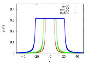
Figure 2: Mean density of real roots $\rho_{n}(x)$ given in Eq. (41) for Weyl polynomials $W_{n}(x)$ (6) as a function of $x$ for different values of $n=50,100$ and $500$.

For $n$ large but finite, the density is uniform like in Eq. (42) up to $|x|\sim\sqrt{n}$ above which it vanishes (see Fig. 2). Indeed, one shows in Appendix B that for $n\gg 1$, one has

$$\rho_{n}(x)\sim\begin{cases}\pi^{-1}\quad,\quad|x|\ll\sqrt{n}\;,\\ \tfrac{\sqrt{n}}{\pi x^{2}}\quad,\quad|x|\gg\sqrt{n}\;.\end{cases}$$ (43)

One notices that this behavior of the density of real roots for Weyl polynomials (43) is similar to the density of real eigenvalues for Ginibre random matrices edelman_ginibre , i.e. random $n\times n$ matices formed from i.i.d. Gaussian entries. Besides, from this scaling form (43) one obtains the number of real roots in the interval $[-x,x]$, $x>0$, in the large $n$ limit as

$$\langle N_{n}[-x,x]\rangle=\int_{-x}^{x}dt\rho_{n}(t)\sim\begin{cases}2x/\pi\;,\;x<\sqrt{n}\\ 2\sqrt{n}/\pi\;,\;x\geq\sqrt{n}\;,\end{cases}$$ (44)

from which one gets the total number of real roots for $n\gg 1$ (see also Ref. leboeuf )

$$\langle N_{n}[-\infty,+\infty]\rangle\sim\frac{2}{\pi}\,\sqrt{n}\;.$$ (45)

To our knowledge, the higher order terms in this large $n$ expansion are not known.

III.1.3 Binomial polynomials

For binomial polynomials, the computation of the density $\rho_{n}(x)$ is straightforward. Indeed, using Eq. (17) together with the formula for the density (21), one obtains

$$\rho_{n}(x)=\sqrt{n}\rho^{B}(x)\quad,\quad\rho^{B}(x)=\frac{1}{\pi(1+x^{2})}\;,$$ (46)

exactly for all $n>1$ edelman ; bleher .

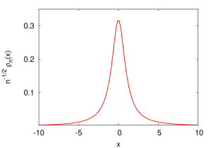
Figure 3: Scaled mean density of real roots $n^{-1/2}\rho_{n}(x)$ as a function of $x$ (46) for binomial polynomials $B_{n}(x)$ (7).

In Fig. 3, we show a plot of $\rho^{B}(x)$ as a function of $x$. This formula (46) yields

$$\langle N_{n}[a,b]\rangle=\int_{a}^{b}\,\rho_{n}(t)\,dt=\frac{\sqrt{n}}{\pi}(\operatorname{ArcTan}{b}-\operatorname{ArcTan}{a})\;,$$ (47)

from which one gets the very simple result (see for instance Ref. edelman )

$$\langle N_{n}[-\infty,+\infty]\rangle=\sqrt{n}\;,\;{\rm exactly\;}\;\forall n\;.$$ (48)

III.2 ”Gap probability” on the real axis

We now study another aspect of the statistical properties of the real roots of these polynomials and focus on the probability $P_{0}([a,b],n)$ that they have no real root on a given interval $[a,b]$. The interval under study will depend on the polynomials $K_{n}(x)$, $W_{n}(x)$ or $B_{n}(x)$.

III.2.1 Results from the correlation function

These polynomials, as a function of $x$, are Gaussian processes and therefore their zero-crossing properties are completely determined by the two-point correlators given in Eq. (15-17).

Generalized Kac polynomials: For these polynomials $K_{n}(x)$, given the singularity of the mean density $\rho_{n}(x)$ around $x=\pm 1$ (see Fig. 1), it is natural to study separately $P_{0}([0,x],n)$, for $x<1$, and $P_{0}([x,\infty],n)$ for $x>1$. We first focus on $P_{0}([0,x],n)$ and reparametrize $K_{n}(x)$ with a change of variable, $x=1-1/t$. One finds that the relevant scaling limit of ${C}_{n}(t,t^{\prime})$ is obtained for $t,t^{\prime},n\to\infty$ keeping $\tilde{t}=t/n$ and $\tilde{t}^{\prime}=t^{\prime}/n$ fixed. In that scaling limit the discrete sum in Eq. (15) can be viewed as a Riemann sum and one finds

$$C_{n}(x,y)\propto n^{d/2}I_{d/2-1}\left(\frac{1}{2\tilde{t}}+\frac{1}{2\tilde{t}^{\prime}}\right)\;,$$ (49)

where $I_{m}(y)$ is defined in Eq. (29). Thus the normalized correlator ${\hat{C}}_{n}(t,t^{\prime})\to{\cal C}(\tilde{t},\tilde{t}^{\prime})$ with the asymptotic behaviors (see Eq. (120))

$${\cal C}(\tilde{t},\tilde{t}^{\prime})\sim\begin{cases}\left(4\frac{{\tilde{t}\tilde{t}^{\prime}}}{(\tilde{t}+\tilde{t}^{\prime})^{2}}\right)^{\tfrac{d}{4}}\,,&\tilde{t},\tilde{t}^{\prime}\ll 1\\ 1\,,&\tilde{t},\tilde{t}^{\prime}\gg 1\;.\end{cases}$$ (50)

Thus this correlator is exactly the same as the one found for diffusion, ${\cal C}(\tilde{t},\tilde{t}^{\prime})=a(\tilde{t},\tilde{t}^{\prime})$ in Eq. (12). Since a Gaussian process is completely characterized by its two-point correlator, we conclude that the diffusion process and the random polynomial are essentially the same Gaussian process and hence have the same zero crossing properties. Therefore, in complete analogy with Eq. (2) we propose the scaling form for generalized Kac polynomials

$$P_{0}([0,x],n)={\cal A}^{-}_{d,n}n^{-\theta(d)}h^{-}(n(1-x))\;,$$ (51)

where ${\cal A}^{-}_{d,n}$, which is independent of $x$, is such that $\lim_{n\to\infty}\log{{\cal A}^{-}_{d,n}}/\log n=0$ and $h^{-}(y)\to 1$ for $y\ll 1$ whereas $h^{-}(y)\sim y^{\theta(d)}$ for $y\gg 1$, where $\theta(d)$ is the persistence exponent associated to the diffusion equation in dimension $d$. Defined in this way (51), $h^{-}(u)$ is a universal function (see below), although the amplitude ${\cal A}^{-}_{d,n}$ is not. Note that $n$ here plays the role of $L^{2}$ in diffusion problem while the variable $1-x$ is the analogue of the inverse time $1/t$.

Similarly, we focus on $P_{0}([x,\infty],n)$, $x>1$, and reparametrize the polynomial with a change of variable, $x=1+1/t$. One finds that the relevant scaling limit of ${C}_{n}(t,t^{\prime})$ is obtained for $t,t^{\prime},n\to\infty$ keeping $\tilde{t}=t/n$ and $\tilde{t}^{\prime}=t^{\prime}/n$ fixed and one obtains

$$C_{n}(x,y)\propto n^{d/2}I_{d/2-1}\left(-\frac{1}{2\tilde{t}}-\frac{1}{2\tilde{t}^{\prime}}\right)\;,$$ (52)

where $I_{m}(y)$ is defined in Eq. (29). Thus ${\hat{C}}_{n}(x,y)\to{\cal C}(\tilde{t},\tilde{t}^{\prime})$ with the asymptotic behaviors (see Eq. (120))

$${\cal C}(\tilde{t},\tilde{t}^{\prime})\sim\begin{cases}\left(4\frac{{\tilde{t}\tilde{t}^{\prime}}}{(\tilde{t}+\tilde{t}^{\prime})^{2}}\right)^{\tfrac{1}{2}}\,,&\tilde{t},\tilde{t}^{\prime}\ll 1\\ 1\,,&\tilde{t},\tilde{t}^{\prime}\gg 1\;,\end{cases}$$ (53)

independently of $d$. Therefore, in complete analogy with Eq. (2) we propose the scaling form for random polynomials

$$P_{0}([x,\infty],n)={\cal A}^{+}_{d,n}n^{-\theta(2)}h^{+}(n(x-1))\;,$$ (54)

where ${\cal A}^{+}_{d,n}$, which is independent of $x$ is such that $\lim_{n\to\infty}\log{{\cal A}^{+}_{d,n}}/\log n=0$ and $h^{+}(y)\to 1$ for $y\ll 1$ whereas $h^{-}(y)\sim y^{\theta(2)}$ for $y\gg 1$.

Using the correlator $\hat{C}_{n}(x,y)$, one shows the statistical independence of the real roots of $K_{n}(x)$ in the four sub-intervals $[-\infty,-1]$, $[-1,0]$, $[0,1]$ and $[1,+\infty]$. Consider for instance the intervals $[0,1]$ and $[1,+\infty]$. Given that the real roots in the interval $[0,+\infty]$ are concentrated, for $n\gg 1$, around $x=1$ we introduce $x=1-1/t$ and $y=1+1/t^{\prime}$ and consider the limit $t,t^{\prime},n\to\infty$. One easily obtains

$$\hat{C}_{n}(1-1/t,1+1/t^{\prime})\propto e^{-n/{\rm Max}(t,t^{\prime})}\;,$$ (55)

which decays to $0$ exponentially for large $n$. Therefore one concludes that the zeros of $K_{n}(x)$ in the sub-intervals $[0,1]$ and $[1,\infty]$ are essentially independent. In a similar way, one shows that the real roots of $K_{n}(x)$ on the four subintervals delimited by $\pm 1$ are statistically independent. Finally combining Eqs (51, 54) together with (55) one obtains the exact asymptotic result for the probability of no real root as

$$P_{0}([-\infty,\infty],n)\propto n^{-2(\theta(d)+\theta(2))}\;.$$ (56)

We conclude this paragraph by presenting a heuristic argument which allows to connect the zero crossing properties of the diffusion equation to the one of the real roots of $K_{n}(x)$. For that purpose, we consider the solution of the diffusion equation with random initial condition (11) and we focus on $\phi(0,t)$, without any loss of generality. Following Ref. hilhorst , one observes that the solid angle integration in that expression can be absorbed into a redefinition of the random field, yielding

$$\phi(0,t)=\frac{S_{d}^{1/2}}{(4\pi t)^{d/2}}\int_{0}^{L}dr\;r^{(d-1)/2}e^{-r^{2}/t}\Psi(r)\;,$$ (57)

where $S_{d}$ is the surface of the $d$-dimensional unit sphere and $\Psi(r)$ is given by hilhorst

$$\Psi(r)=S_{d}^{-1/2}r^{-\tfrac{1}{2}(d-1)}\lim_{\Delta r\to 0}\frac{1}{\Delta r}\int_{r<x<r+\Delta r}d{\mathbf{x}}\;\psi(\mathbf{x})\;,$$ (58)

which is thus a random Gaussian variable of zero mean and correlations $\langle\Psi(r)\Psi(r^{\prime})\rangle=\delta(r-r^{\prime})$. Performing the change of variable $u=r^{2}$ in Eq. (57), one obtains

$$\phi(0,t)\propto\int_{0}^{L^{2}}du\;u^{\tfrac{d-2}{4}}e^{-u/t}\tilde{\Psi}(u)\;,\;\langle\tilde{\Psi}(u)\tilde{\Psi}(u^{\prime})\rangle=\delta(u-u^{\prime})\;.$$ (59)

On the other hand, if we focus on the real zeros of $K_{n}(x)$ in the interval $[0,x]$ with $x<1$, we know that these zeros accumulate in the vicinity of $x=1$. Therefore, in terms of $x=1-1/t$ one has

$$K_{n}(x)\sim a_{0}+\sum_{i=1}^{n}i^{(d-2)/4}e^{-i/t}a_{i}\;.$$ (60)

By approximating the discrete sum in the above expression (60) by an integral, one sees that $K_{n}(x)$ is similar to the solution of the diffusion equation in Eq. (59) where $L^{2}$ is replaced by $n$ and $1-x$ by $1/t$. Therefore one understands qualitatively why the zero crossing properties of these two processes coincide.

Weyl polynomials: To analyse the correlation function in Eq. (16) in the large $n$ limit we write it as

$$C_{n}(x,y) = \langle W_{n}(x)W_{n}(y)\rangle=\sum_{i=0}^{n}\frac{(xy)^{i}}{i!}=e^{xy}\frac{\Gamma(n+1,xy)}{\Gamma(n+1)}\;,$$ (61)

where the last equality can easily be obtained using the recursion relation $\Gamma(n+1,z)=n\Gamma(n,z)+e^{-z}z^{n}$. The behavior of $\Gamma(n,z)$ for large $n$ is analysed in detail in Appendix B. From the results obtained in Eq. (124, 125), one sees that the correlation function $C_{n}(x,y)$ in Eq. (61) behaves differently for $xy<n$ and $xy>n$.

For $xy<n$, Eq. (124) shows that $\Gamma(n+1,xy)\to\Gamma(n+1)$ for large $n$ so that one finds that $\hat{C}_{n}(x,y)\to{\cal C}(x,y)$ with

$${\cal C}(x,y)=\exp{[-\tfrac{1}{2}(x-y)^{2}]}\;.$$ (62)

Interestingly Eq. (62) shows that inside the interval $[-\sqrt{n},\sqrt{n}]$, $W_{n}(x)$ is exactly the GSP characterizing the zero crossing properties of the diffusion field in the limit of infinite dimension $d\to\infty$ (14). Therefore one expects $P_{0}([-x,x],n)$, the probability that $W_{n}(x)$ has no real root in the interval $[-x,x]$, with $1\ll x\leq\sqrt{n}$, to behave as

$$P_{0}([-x,x],n)\propto\exp{(-2\theta_{\infty}x)}\;.$$ (63)

For $xy>n$, the behavior of $C_{n}(x,y)$ is quite different. Indeed, using the asymptotic behavior in Eq. (125), one shows that the relevant scaling limit is obtained for $x,y,n\to\infty$ keeping $\tilde{x}=x/\sqrt{n}$ and $\tilde{y}=y/\sqrt{n}$ fixed such that $\hat{C}_{n}(x,y)\to{\cal C}(\tilde{x},\tilde{y})$ with

$${\cal C}(\tilde{x},\tilde{y})=\frac{\sqrt{\tilde{x}^{2}-1}\sqrt{\tilde{y}^{2}-1}}{\tilde{x}\tilde{y}-1}\quad,\;\tilde{x}\tilde{y}\geq 1\;,\;.$$ (64)

Performing the change of variable $x\to\tilde{x}=\sqrt{n}+1/(\sqrt{n}\tilde{t})$ one easily obtains that ${\cal C}(\tilde{t},\tilde{t}^{\prime})$ behaves like in Eq. (53). Therefore, by analogy with Eq. (54), one deduces that, for $0<x-\sqrt{n}\ll 1$, $n\gg 1$ keeping $\sqrt{n}(x-\sqrt{n})$ fixed, one has

$$P_{0}([x,\infty],n)\propto n^{-\tfrac{\theta(2)}{2}}w(\sqrt{n}(x-\sqrt{n}))\;,$$ (65)

where $w(u)\sim c^{\rm st}$ for $u\ll 1$ and $w(u)\propto u^{\theta(2)}$ for $u\gg 1$. In addition, following the arguments presented above (see Eq. (55)), one shows that these two outer-intervals $[-\infty,-\sqrt{n}]$ and $[\sqrt{n},+\infty]$ are statistically independent, such that

$$P_{0}([-\infty,-\sqrt{n}]\cup[\sqrt{n},+\infty],n)\propto n^{-\theta(2)}\;.$$ (66)

However, given the behavior of the correlator ${\cal C}(x,y)$ for $xy>n$ in Eq. (62) the inner and outer intervals are not independent and the probability of no root on the real axis is not the product of the probabilities in Eq. (63) evaluated in $x=\sqrt{n}$ and the the one in Eq. (66) : the effect of these correlations will be discussed below.

Binomial polynomials: In that case, one can extract information directly from the correlation function in Eq. (17) by focusing in the limit $x,y\to 0$. In that limit the normalized correlation function $\hat{C}_{n}(x,y)$ is given by

$$\hat{C}_{n}(x,y)=\frac{(1+x\,y)^{n}}{[(1+x^{2})(1+y^{2})]^{\tfrac{n}{2}}}\sim\exp{\left[-\tfrac{n}{2}(x-y)^{2}\right]}\;,\;x,y\ll 1\;.$$ (67)

Thus in the large $n$ limit, the probability $P_{0}([a,b],n)$ that binomial polynomials have no real root in the interval $[a,b]$ with $a<b\ll 1$, $n^{-\tfrac{1}{2}}\ll b-a$ behaves like

$$P_{0}([a,b],n)\propto\exp{\left[-\theta_{\infty}\sqrt{n}(b-a)\right]}\;,\;a<b\ll 1\;,\;n^{-\tfrac{1}{2}}\ll b-a\;,$$ (68)

which is an exact statement. However it is a more difficult task to obtain the behavior of $P_{0}([a,b],n)$ for an arbitrary interval $[a,b]$ and eventually obtain the probability of no root on the entire real axis for this class of polynomials (7) : this will be achieved in the next sections.

To conclude this paragraph, we have shown that the analysis of the correlation function $C_{n}(x,y)$ yields important exact results for the gap probabilities. Indeed, for generalized Kac polynomials, we obtained the important results in Eq. (51) and Eq. (54) which yield the exact result in Eq. (56). For Weyl polynomials the study of the correlation function allowed us to obtain the results in Eq. (63) and Eq. (65). Finally, for Binomial polynomials we obtained, from the correlation funtion, the asymptotic behavior in Eq. (68), which will be useful in the following.

III.2.2 Mean-Field description : Poisson approximation

To calculate the gap probabilities and the associated scaling functions, we first develop a very simple mean field theory. This theory, albeit approximate as it neglects the correlations between zeros, is simple, intuitive and qualitatively correct. We will see later how one can improve systematically this mean field theory to get answers that are even quantitatively accurate. As a first step, we neglect the correlations between the real roots and simply consider that these roots are randomly and independently distributed on the real axis with some local density $\rho_{n}(x)$ at point $x$. Within this approximation the probability $P_{k}([a,b],n)$ that these polynomials have exactly $k$ real roots satisfies the equation

$$\frac{\partial P_{k+1}([a,b],n)}{\partial b}=\rho_{n}(b)[P_{k}([a,b],n)-P_{k+1}([a,b],n)]\;,$$ (69)

together with the normalization condition $\sum_{k\geq 0}P_{k}([a,b],n)=1$ and $P_{k}([a,b],n)=\delta_{k,0}$ when $a=b$. In the large $n$ limit (where one can omit the constraint $P_{k>n}([a,b],n)=0$), $P_{k}([a,b],n)$ is given by a non-homogeneous Poisson distribution

$$P_{k}([a,b],n)=\frac{\mu^{k}}{k!}\,e^{-\mu}\;,\;\mu=\langle N_{n}[a,b]\rangle=\int_{a}^{b}\rho_{n}(x)dx\;,$$ (70)

which clearly satisfies Eq. (69). In particular, this mean field approximation (70) yields the gap probability

$$P_{0}([a,b],n)=\exp{\left(-\langle{N}_{n}[a,b]\rangle\right)}=\exp{\left(-\int_{a}^{b}\rho_{n}(x)\;dx\right)}\;.$$ (71)

When applied to Generalized Kac polynomials $K_{n}(x)$, for which we obtained $\langle{N}_{n}[0,x]\rangle$ in Eq. (35), this mean-field approximation (71) yields in the scaling limit $n\to\infty$, $1-x\to 0$, $n(1-x)>0$ fixed

$$P_{0}([0,x],n)={\cal A}_{d,n}^{-}n^{-\tfrac{1}{2\pi}\sqrt{\tfrac{d}{2}}}\exp{\left[\eta_{-}(n(1-x))\right]}\;,$$ (72)

where, from Eq. (32), $\log{\cal A}_{d,n}^{-}=o(\log{n})$. This mean-field approximation thus yields the correct scaling from for $P_{0}([0,x],n)$ as in Eq. (51), with the non trivial predictions for the exponent and scaling function

$$\theta^{\rm MF}(d)=\frac{1}{2\pi}\sqrt{\frac{d}{2}}\hskip 5.69046pt,\hskip 5.69046pth^{-}(u)=\exp{\left(\int_{0}^{u}dy\rho^{K}(y)\right)}\;,$$ (73)

with the asymptotic behavior $h^{-}(u)\sim 1$ for $u\ll 1$ and, using the asymptotic behavior obtained in Eq. (37), $h^{-}(u)\sim u^{\theta^{\rm MF}(d)}$.

Similarly, this mean-field approximation applied to Weyl polynomials $W_{n}(x)$, for which we obtained $\langle{N}_{n}[-x,x]\rangle$ in Eq. (44), yields the scaling form

$$P_{0}([-x,x],n)\sim\begin{cases}\exp{(-2x/\pi)}\;,\;x<\sqrt{n}\\ \exp{(-2\sqrt{n}/\pi)}\;,\;x\geq\sqrt{n}\;.\end{cases}$$ (74)

Notice that this mean-field approximation gives an approximation of $\theta^{\rm MF}_{\infty}=\pi^{-1}=0.31831...$ (see Eq. (63)), which is consistent, using the relation $\theta(d)=2^{-3/2}\theta_{\infty}\sqrt{d}$ for large $d$, with Eq. (73).

Finally, if one uses this mean-field approximation to study binomial polynomials $B_{n}(x)$, one obains, using the expression $\langle{N}_{n}[a,b]\rangle$ given in Eq. (47)

$$P_{0}([a,b],n)=\exp{\left[-\frac{\sqrt{n}}{\pi}(\operatorname{ArcTan}{a}-\operatorname{ArcTan}{b})\right]}\;,$$ (75)

which again, according to Eq. (68), gives the mean-field approximation for $\theta^{\rm MF}_{\infty}=\pi^{-1}$, as above.

III.2.3 Beyond Mean-Field : a systematic approach

We will now show that this mean field approximation (71) can actually be improved systematically. For that purpose, one considers the probability $P_{k}([a,b],n)$ that such polynomials as in Eq. (3, 6, 7) have exactly $k$ real roots in the interval $[a,b]$. Following Ref. satya_partial , one introduces the generating function

$$\hat{P}_{n}(p,[a,b])=\sum_{k=0}^{\infty}p^{k}P_{k}([a,b],n)\;,$$ (76)

where $\hat{P}_{n}(p,[a,b])$ can be interpreted as a persistence probability with partial survival satya_partial . For a smooth process, it turns out that $\hat{\theta}_{n}(p,[a,b])=-\log{(\hat{P}_{n}(p,[a,b]))}$ depends continuously on $p$ : this was shown exactly for the random acceleration process (see Eq. (106) below) and approximately using the IIA - and further checked numerically - for the diffusion equation with random initial conditions satya_partial . Thus one has

$$\hat{\theta}_{n}(p,[a,b])=-\log{(\hat{P}_{n}(p,[a,b]))}=-\sum_{r=1}^{\infty}\frac{(\log{(p)})^{r}}{r!}\langle N^{r}_{n}([a,b])\rangle_{c}\;,$$ (77)

where the notation $\langle...\rangle_{c}$ stands for a connected average. Here we are interested in $\hat{P}_{n}(p=0,[a,b])=P_{0}([a,b],n)$ and the idea, given that $\hat{\theta}_{n}(p=1,[a,b])=0$ is to expand $\hat{\theta}_{n}(p,[a,b])$ around $p=1$ in an $\epsilon$-expansion with $p=1-\epsilon$. This yields

$$\hat{\theta}_{n}(1-\epsilon,[a,b])=\sum_{r=1}^{\infty}{\mathfrak{a}}_{r,n}([a,b])\epsilon^{r}\;,$$ (78)

where ${\mathfrak{a}}_{r,n}([a,b])$ are linear combinations of the cumulants $\langle N^{m}_{n}[a,b]\rangle_{c}$, with $m\leq r$. For instance,

$${\mathfrak{a}}_{1,n}([a,b])=\langle N_{n}[a,b]\rangle\;,\;{\mathfrak{a}}_{2,n}([a,b])=\tfrac{1}{2}\left(\langle N_{n}[a,b]\rangle-\langle N^{2}_{n}[a,b]\rangle_{c}\right)\;,$$ (79)

$${\mathfrak{a}}_{3,n}([a,b])=\left(\frac{\langle N_{n}[a,b]\rangle}{3}-\frac{\langle N^{2}_{n}[a,b]\rangle_{c}}{2}+\frac{\langle N^{3}_{n}[a,b]\rangle_{c}}{6}\right)\;.$$

Thus one sees that if one restricts the $\epsilon$-expansion in Eq. (78) to first order, and set $\epsilon=1$, one recovers the mean-field approximation (71), using ${\mathfrak{a}}_{1,n}([a,b])=\langle{N}_{n}[a,b]\rangle$. Higher order terms in this $\epsilon$-expansion allow to improve systematically this mean-field approach.

Kac polynomials for $d=2$: We first illustrate this $\epsilon$ expansion for Kac polynomials $K_{n}(x)$ for $d=2$ where we compute $\hat{\theta}_{n}(1-\epsilon,[0,x])$ up to order ${\cal O}(\epsilon^{2})$. In that purpose, we compute ${\mathfrak{a}}_{2,n}([0,x])$. In Appendix C, we show that in the scaling limit $(1-x)\to 0$, and $n\to\infty$ keeping the product $n(1-x)$ fixed one has, similarly to the Eq. (35) for the first moment,

$$\langle N^{2}_{n}[0,x]\rangle_{c}=\langle N^{2}_{n}[0,1]\rangle_{c}-\nu_{-}(n(1-x))$$ (80)

where $\nu_{-}(y)$, given in Eq. (141), is such that $\nu_{-}(y)\to 0$ for $y\ll 1$ and

$$\nu_{-}(y)\sim\left(\frac{1}{\pi}-\frac{2}{\pi^{2}}\right)\log{y}\;,\;y\gg 1\;.$$ (81)

Notice that $\langle N^{2}_{n}[0,1]\rangle_{c}$ in Eq. (80) has been computed in Ref. maslova , yielding for large $n$

$$\langle N^{2}_{n}[0,1]\rangle_{c}=\left(\frac{1}{\pi}-\frac{2}{\pi^{2}}\right)\log{n}+o(\log{n})\;,$$ (82)

although higher order terms in this large $n$ expansion are not known. Combining Eq. (78, 79, 80) together with the expression for $\nu_{-}(y)$ in Eq. (141), one obtains in the scaling limit

$$\hat{\theta}_{n}(1-\epsilon,[0,x])=\left(\epsilon+\tfrac{\epsilon^{2}}{2}\right)\langle N_{n}([0,1])\rangle-\tfrac{\epsilon^{2}}{2}\langle N_{n}([0,1])^{2}\rangle_{c}$$ (83)

$$-\epsilon\int_{0}^{y}du\,\rho^{K}(u)+\epsilon^{2}\int_{0}^{y}du_{1}\int_{u_{1}}^{\infty}du_{2}\left(\tilde{\cal K}(u_{1},u_{2})-\rho^{K}(u_{1})\rho^{K}(u_{2})\right)+{\cal O}(\epsilon^{3})\;,$$

with $y=n(1-x)$. In this Eq. (83), $\rho^{K}(u)$ is given in Eq. (31), and $\tilde{\cal K}(u_{1},u_{2})$, which we study in detail in Appendix C, is essentially the two-point correlation function of real roots inside the peak of the density around $x=1$ (see right panel of Fig. 1). Setting $\epsilon=1$ in this expression to order ${\cal O}(\epsilon^{2})$ (83) one obtains, for $d=2$

$$P_{0}([0,x],n)={\cal A}^{-}_{d,n}n^{-\theta(2)}h^{-}(n(x-1))\;,\;\theta(2)=\frac{\pi+4}{4\pi^{2}}=0.180899...\;,$$ (84)

$$h^{-}(y)=\exp{\left(\int_{0}^{y}du\,\rho^{K}(u)-\int_{0}^{y}du_{1}\int_{u_{1}}^{\infty}du_{2}\left(\tilde{\cal K}(u_{1},u_{2})-\rho^{K}(u_{1})\rho^{K}(u_{2})\right)\right)}\;,$$ (85)

with $\log{{\cal A}^{-}_{d,n}}=o(\log{n})$ (see Eqs (32, 82)). Note that the value of the exponent $\theta(2)$ up to second order as given in this Eq. (84) was computed in Ref. satya_partial . In the next sections, we will show, using numerics, that this second order calculation (84) is a true improvement upon the mean-field approximation (73).

Weyl polynomials: We now compute $\hat{\theta}_{n}(1-\epsilon,[-x,x])$, $x<\sqrt{n}$ for Weyl polynomials up to order ${\cal O}(\epsilon^{2})$. In that purpose we compute ${\mathfrak{a}}_{2,n}([-x,x])$. In Appendix D, one shows that for $x<\sqrt{n}$ fixed and $n\gg 1$, one has

$$\langle N^{2}_{n}[-x,x]\rangle_{c}=\nu(x)\;,$$ (86)

with $\nu(x)$ given in Eq. (163). Combining Eq. (78, 79, 86) together with the expression for $\nu(x)$ in Eq. (163), one obtains for large $n$

$$\hat{\theta}_{n}(1-\epsilon,[-x,x])=\epsilon\frac{2x}{\pi}+2\epsilon^{2}\int_{0}^{x}ds(s-x)(\tilde{\cal W}(s)-\pi^{-2})+{\cal O}(\epsilon^{3})\;,$$ (87)

where $\tilde{\cal W}(s)$, given in Eq. (160), is the two point correlation function of real roots in the interval $[-\sqrt{n},\sqrt{n}]$. Setting $\epsilon=1$ in this expression up to order ${\cal O}(\epsilon^{2})$ (87), one obtains, for $x<\sqrt{n}$

$$P_{0}([-x,x],n)=\exp{\left(-\frac{2x}{\pi}-\int_{0}^{2x}ds(s-2x)(\tilde{\cal W}(s)-\pi^{-2})\right)}\;.$$ (88)

Using Eq. (165), one obtains its large $x$ behavior as in Eq. (63) with the value of $\theta_{\infty}$ up to order ${\cal O}(\epsilon^{2})$

$$\theta_{\infty}=\frac{1}{\pi}-\int_{0}^{\infty}ds(\tilde{\cal W}(s)-\pi^{-2})=0.386471...\;,$$ (89)

which should be compared with the numerical value $\theta_{\infty,{\rm sim}}=0.417(3)$ newman_diffusion .

If we focus instead on the outer intervals $[-\infty,-\sqrt{n}]\cup[\sqrt{n},\infty]$, this $\epsilon$ expansion is essentially similar to the one performed for Kac polynomials and $d=2$, given the behavior of the correlator in Eq. (64). More interestingly, if we are interested in the computation of the probability of no root on the real axis, this $\epsilon$ expansion is able to take into account (perturbatively) the correlations between the inner and outer intervals, which, as discussed below Eq. (66), can be seen in the correlation function (62). Doing so, one obtains that

$$P_{0}([-\infty,\infty],n)=P_{0}([-\sqrt{n},\sqrt{n}],n)P_{0}([-\infty,-\sqrt{n}]\cup[\sqrt{n},\infty],n)\mathfrak{p}_{n}\;,$$ (90)

where the computation of $\mathfrak{p}_{n}$ is similar to the one carried out in Appendix D where the quantity ${\cal W}_{n}(t_{1},t_{2})$ in Eq. (154) involves $t_{1}\in[-\sqrt{n},\sqrt{n}]$ and $t_{2}\in[-\infty,-\sqrt{n}]\cup[\sqrt{n},\infty]$ such that $t_{1}t_{2}<1$. The computation up to order ${\cal O}(\epsilon^{2})$ shows that $\mathfrak{p}_{n}\propto n^{\tau}$ with $\tau>0$. Therefore, on the basis of this result together with Eqs (63, 66), one expects

$$P_{0}([-\infty,\infty],n)\sim n^{-\gamma}\exp{(-2\theta_{\infty}\sqrt{n})}\;,$$ (91)

where the exponent $\gamma$ is a priori unknown. Below, we will confront this statement with numerical simulations.

Binomial polynomials: We now focus on $\hat{\theta}_{n}(1-\epsilon,n)$ for binomial polynomials. In Ref. bleher , it was shown that for large $n$ and all $a,b>n^{-\tfrac{1}{2}}$

$$\langle N^{2}_{n}[a,b]\rangle_{c}\propto\beta_{2}\langle N_{n}[a,b]\rangle\;,$$ (92)

where $\beta_{2}$ is a constant, independent of $n,a$ and $b$. It has an analytic expression in term of an integral involving elementary functions, with $\beta_{2}=0.571731...$. This expression (92) yields in the large $n$ limit, ${\mathfrak{a}}_{2,n}([a,b])~{}=~{}(1/2~{}-~{}\beta_{2}~{})~{}\langle N_{n}[a,b]\rangle$ which together with the asymptotic behavior in Eq. (68) and the cumulant expansion of Eq. (78) allows to compute $\theta_{\infty}$ up to order ${\cal O}(\epsilon^{2})$. We have checked that this coincides with the one obtained in Eq. (89). More generally, one expects that for all integer $m>0$

$$\langle N^{m}_{n}[a,b]\rangle_{c}\propto\beta_{m}\langle N_{n}[a,b]\rangle\;,$$ (93)

where $\beta_{m}$ is a constant, independent of $n,a$ and $b$ and in Appendix E we explicitly show the mechanism leading to this relation (93) for $k=3$. From these relations (93) and the structure of the cumulant expansion in Eq. (78), one expects that $P_{0}([a,b],n)\propto\exp{[-\omega\langle N_{n}[a,b]\rangle]}$, where $\omega$ is a linear combination of the coefficients $\beta_{m}$. Finally, this expression has to match the exact asymptotic behavior of $P_{0}([a,b],n)$ for $a<b\ll 1$ and $n^{-\tfrac{1}{2}}\ll b-a$ derived in Eq. (68). Thus one has $\omega=\pi\theta_{\infty}$ so that one obtains the exact result

$$P_{0}([a,b],n)\propto\exp{\left[-\sqrt{n}\theta_{\infty}(\operatorname{ArcTan}{b}-\operatorname{ArcTan}{a})\right]}\;,$$ (94)

from which we obtain the exact expression for the probability of no real root for $B_{n}(x)$ in the large $n$ limit as

$$P_{0}([-\infty,+\infty],n)\propto\exp{\left(-\sqrt{n}\pi\theta_{\infty}\right)}\;.$$ (95)

Below, we check this analytical result (94) using numerical simulations.

III.2.4 Numerical results

Kac polynomials: We first focus on the interval $[0,1]$ and check numerically the scaling forms for $P_{0}([0,x],n)$ in Eq. (2) for $K_{n}(x)$ and for different values of $d$. In each case, this probability is obtained by averaging over $10^{4}$ realizations of the random variables $a_{i}$’s in Eq. (3), drawn independently from a Gaussian distribution of unit variance. In Ref. us_prl , we already presented numerical results for $P_{0}([0,x],n)$ in $d=2$ and we also checked that $P_{0}([0,x],n)\propto n^{-\theta(2)}$ with $\theta(2)=0.187(1)$. In the left panel of Fig. 4, we show a plot of $\log[P_{0}([0,x],n)/P_{0}([0,1],n)]$ for $d=2$ as a function of the scaled variable $n(1-x)$ for different values of $n$. According to Eq. (2), together with the good collapse of the curves for different values of $n$, this allows for a numerical computation of the scaling function $h^{-}(y)$. We have checked that different distributions of the random coefficients either $a_{i}=\pm 1$ or rectangular distribution yield the same scaling function $h^{-}(y)$, suggesting that this function is indeed universal. On the same figure, the dotted line is the result of Mean Field approximation (73), or first order in the $\epsilon$ expansion, and the solid line is the analytical result of the second order calculation obtained in Eq. (84). In both cases, the integrals involved were evaluated numerically using the Mathematica. As expected one observes on this plot that the Mean Field calculation is only in qualitative agreement with the numerical results, we recall in particular that $\theta_{\rm MF}(2)=1/2\pi=0.159155...$. Interestingly, one sees that the second order calculation is a clear improvement over the Mean Field calculation which is in quite good agreement with the numerical results for the scaling function, in particular, $\theta(2)=(\pi+4)/4\pi^{2}=0.180899...$. We have checked that this scaling (2) holds for other values of $d$. In the right panel of Fig. 4, we show a plot of $n^{\theta(3)}P_{0}([0,x],n)$ for $d=3$ and $\theta(3)=0.238(4)$ as a function of $n(1-x)$ for different degrees $n=256,512,1024$. Again, the value of $\theta(3)=0.238(4)$ for which one obtains the best collapse of the curves for different values of $n$ is in good agreement with the values of $\theta(3)$ found for the diffusion equation persist_diffusion ; newman_diffusion .

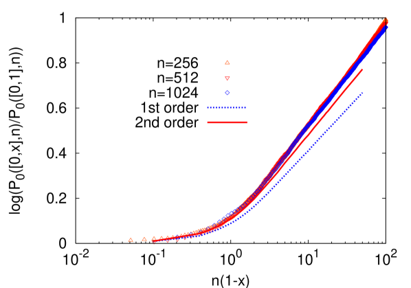
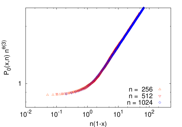
Figure 4: Left : Plot of $\log[P_{0}([0,x],n)/P_{0}([0,1],n)]$ for Kac polynomials $K_{n}(x)$ and $d=2$ as a function of $n(1-x)$ for different degrees $n=256,512,1024$. The dotted is the result of the Mean Field prediction (73) and the solid line the result of the second order calculation in the $\epsilon$ expansion (83). Right : Plot of $n^{\theta(3)}P_{0}([0,x],n)$ on a log-log scale for Kac polynomials $K_{n}(x)$ and $d=3$ with $\theta(3)=0.238(4)$ as a function of $n(1-x)$ for different degrees $n=256,512,1024$.

We have also checked numerically our results for the gap probability in the outer intervals (54). For that purpose, we notice that $P_{0}([x,\infty],n)=\overline{P}_{0}([0,1/x],n)$, which is easier to compute numerically, where $\overline{P}_{0}([a,b],n)$ is the gap probability associated to the polynomial $\overline{K}_{n}(x)$ defined such that $K_{n}(x)=x^{n}\overline{K}_{n}(1/x)$ with

$$\overline{K}_{n}(x)=\sum_{i=0}^{n-1}a_{n-i}(n-i)^{\tfrac{d-2}{4}}x^{i}+a_{0}\,x^{n}\;.$$ (96)

Thus, from Eq. (54) one expects that for $0<1-x\ll 1$, and $n\gg 1$, keeping the product $n(1-x)$ fixed one has

$$\overline{P}_{0}([0,x],n)\propto n^{-\theta(2)}h^{+}(n(1-x))\;,$$ (97)

independently of $d$. In Fig. 5, we show a plot of $n^{\theta(2)}\overline{P}_{0}([0,x],n)$ as a function of $n(1-x)$ for $d=3$ and for different values of $n=128,256,512,1024$. Again, the good collapse obtained for $\theta(2)=0.1875$ corroborates the validity of the scaling in Eqs (54, 97).

Figure 5: Plot of $n^{\theta(2)}\overline{P}_{0}([0,x],n)$ on a log-log scale, where $\overline{K}_{n}(x)$ is defined in Eq. (96) as a function of $n(1-x)$ for $d=3$ and for different values of $n=128,256,512,1024$.

Weyl polynomials: We first focus on the inner interval $[-\sqrt{n},\sqrt{n}]$ and compute numerically the gap probability $P_{0}([-x,x],n)$ for $x<\sqrt{n}$. Here also, this probability was computed by averaging over $10^{4}$ different realizations of the random coefficients $a_{i}$’s. In the left panel of Fig. 6, we show a plot of $[\log P_{0}([-x,x],n)]n^{-1/2}$ as a function of $x/\sqrt{n}<1$ for different values of $n=40,90$ and $150$. According to our prediction in Eq. (63), $P_{0}([-x,x],n)$ behaves exponentially for large $x$. From the slope of the straight line in the left panel of Fig. 6, one extracts $2\theta_{\infty}=0.845(3)$, in good agreement with previous numerical estimates from the persistence probability for the diffusion equation in large dimension persist_diffusion ; newman_diffusion . On the same figure, we have also plotted with a dotted line the result from the Mean Field approximation (74) and with a solid line the result up to second order in the $\epsilon$ expansion in Eq. (87). Again, the second order term allows to improve significantly the Mean Field prediction. We recall the estimate up to order ${\cal O}(\epsilon^{2})$, $2\theta_{\infty}=0.7729...$ from Eq. (89). We now focus on the outer intervals $[-\infty,-\sqrt{n}]$ and $[\sqrt{n},+\infty]$. In the right panel of Fig. 6, we plot $n^{\theta(2)}P_{0}([-x,-\sqrt{n}]\cup[\sqrt{n},x],n)$ as a function of $x/\sqrt{n}>1$ for different degrees $n=20,40$ and $90$. The fact that the curves for different $n$ collapse on a single master curve is in agreement with the scaling proposed in Eq. (66).

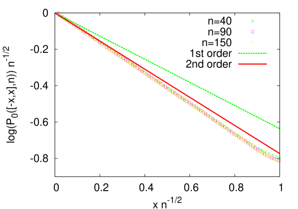
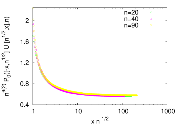
Figure 6: Left : Plot of $[\log P_{0}([-x,x],n)]n^{-1/2}$ for Weyl polynomials $W_{n}(x)$ (6) as a function of $x/\sqrt{n}<1$ for different values of $n=40,90$ and $150$. The dotted line is the result of the Mean Field approximation whereas the solid one is the result of the expansion up to order ${\cal O}(\epsilon^{2})$ in Eq. (87). Right : Plot of $n^{\theta(2)}P_{0}([-x,-\sqrt{n}]\cup[\sqrt{n},x],n)$ as a function of $x/\sqrt{n}>1$ for different degrees $n=20,40$ and $90$.

Finally, we computed the gap probability on the full real axis. In the right panel Fig. 7, we plot $[\log(n^{\gamma}P_{0}([-x,x],n))]n^{-1/2}$ as a function of $x/\sqrt{n}$ for different values of $n=40,90$ and $150$. The exponent $\gamma=0.10(1)$, which is the only fitting parameter is fixed to obtained the best collapse of the different curves in the large $x/\sqrt{n}$ limit. The solid line has a slope $-2\theta_{\infty}=0.845$, which is also the value reached by $\log(n^{\gamma}P_{0}([-x,x],n))n^{-1/2}$ for large $x$. This fact is in complete agreement with the scaling proposed in Eq. (91). The fact that $\gamma<\theta(2)$ arises from the correlations between the inner and outer intervals.

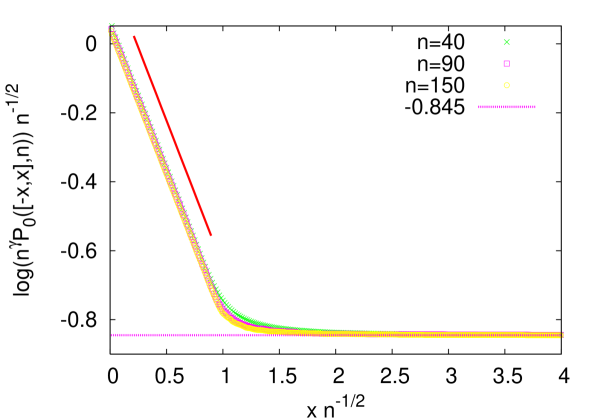
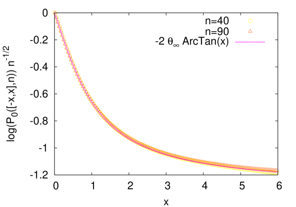
Figure 7: Left : Plot of $[\log(n^{\gamma}P_{0}([-x,x],n))]n^{-1/2}$ for Weyl polynomials $W_{n}(x)$ (6) as a function of $x/\sqrt{n}$ for different values of $n=40,90$ and $150$. Here $\gamma=0.10(1)$ and the solid line has slope $-0.845$. Right : Plot of $[\log P_{0}([-x,x],n)]n^{-1/2}$ for binomial polynomials $B_{n}(x)$ (7) as a function of $x$ for different values of $n=40$ and $90$. The solid line is the exact result in Eq. (94) with $\theta_{\infty}=0.42(1)$, which is the only fitting parameter here.

Binomial polynomials: Finally, we have checked the exact result in Eq. (94) for binomial polynomials (7). For that purpose, we have computed numerically $P_{0}([-x,x],n)$ by averaging over $10^{5}$ different realizations of the random coefficients $a_{i}$’s. In the right panel of Fig. 7, we show a plot of $[\log P_{0}([-x,x],n)]n^{-1/2}$ as a function of $x$ for different values of $n=40$ and $90$. The solid line is the analytic prediction from Eq. (94) with $\theta_{\infty}=0.42(1)$, consistent with our previous estimates from Weyl polynomials (see left panel of Fig. 7). The good agreement with the numerics confirms also the exact result for the probability that these polynomials have no real root on the real axis in Eq. (95).

III.3 Probability of $k$ real roots : large deviation function

We now generalize our analysis and study the probability $P_{k}([a,b],n)$ that such polynomials (3, 6, 7) have exactly $k$ real roots dembo in a given interval $[a,b]$.

III.3.1 Mean field approximation : Poisson approximation

One first considers the Mean Field approximation introduced above where one assumes that the real roots are totally independent and randomly distributed with density $\rho_{n}(x)$. This leads to Eq. (70)

$$P_{k}([a,b],n)=\frac{\langle N_{n}[a,b]\rangle^{k}}{k!}e^{-\langle N_{n}[a,b]\rangle}\;.$$ (98)

If we focus on the limit $n\gg k\gg 1$, keeping the ratio $y=k/\langle N_{n}[a,b]\rangle$ fixed, one has

$$\log P_{k}([a,b],n)\sim-\langle N_{n}[a,b]\rangle\;\varphi_{\rm MF}\left(\frac{k}{\langle N_{n}[a,b]\rangle}\right)\,,\,\varphi_{\rm MF}(y)=1+y\log{y}-y\;,$$ (99)

where we have used the Stirling’s formula $\log{(k!)}=(k+\tfrac{1}{2})\log k-k+{\cal O}(1)$. We will see below (through scaling analysis as well as numerics) that this Mean Field approximation provides the correct scaling form for $P_{k}([a,b],n)$ (although the exact computation of $\varphi(y)$ certainly demands a more sophisticated analysis). Let us present the consequences of this scaling form in Eq. (99) for the different polynomials under study.

Kac polynomials: Let us define $q_{k}(n)=P_{k}([0,1],n)$. In that case, we have seen in Eq. (32) that $\langle N_{n}([0,1])\rangle~{}\sim~{}\tfrac{1}{2\pi}\sqrt{\tfrac{d}{2}}\log n$ so that one expects the scaling form

$$\log q_{k}(n)\propto-\log{n}\,\varphi\left(2\pi\sqrt{\frac{2}{d}}\frac{k}{\log n}\right)\;.$$ (100)

For the special case of Kac polynomials ($d=2$), this scaling form, in the neighborhood of $k=\log n/2\pi$, is consistent with the rigorous result maslova that in this neighborhood $q_{k}(n)$ is a Gaussian with mean $\log n/2\pi$ and variance $V_{n}~{}\sim~{}(\tfrac{1}{\pi}~{}-~{}\tfrac{2}{\pi^{2}})\log n$ (82) in the large $n$ limit.

Weyl’s polynomials: Let us define $q_{k}(n)=P_{k}([-\infty,\infty],n)$. According to Eq. (45), which tells us that $\langle N_{n}[-\infty,\infty]\rangle\sim(2/\pi)\sqrt{n}$, and the scaling form in Eq. (99) one expects

$$\log q_{k}(n)\propto-\sqrt{n}\,\varphi\left(\frac{\pi}{2}\frac{k}{\sqrt{n}}\right)\;.$$ (101)

Binomial polynomials: Let us define similarly $q_{k}(n)=P_{k}([-\infty,+\infty],n)$. In that case, according to Eq. (48) which tells us that $\langle N_{n}[-\infty,\infty]\rangle=\sqrt{n}$, and the scaling form in Eq. (99) one expects

$$\log q_{k}(n)\propto-\sqrt{n}\,\varphi\left(\frac{k}{\sqrt{n}}\right)\;.$$ (102)

In the following, we will check these scaling forms (100-102) numerically.

III.3.2 A more rigorous approach for a smooth Gaussian stationary process

We illustrate this approach on the diffusion equation with random initial conditions (1), which is the underlying stochastic process describing the statistics of real roots of these random polynomials. We thus consider the probability $p_{k}(t,L)$ that the diffusing field $\phi({\mathbf{x}},t)$ crosses zero exactly $k$ times up to time $t$. Let us first consider the regime $1~{}\ll~{}t~{}\ll~{}L^{2}$. In this regime, $p_{k}(t,L)$ is given by the probability ${\cal P}_{k}(T)$ that $X(T)$ crosses zero exactly $k$ times where $X(T)$ is a GSP with correlations $a(|T-T^{\prime}|)=[{\rm cosh}(|T-T^{\prime}|/2)]^{-d/2}$, where $T=\log t$. Since, $a(T)=1-\tfrac{d}{16}T^{2}+o(T^{2})$ for small $T$, this GSP is a smooth process with a finite density of zero crossings given by the Rice’s formula $\mu=[-{a^{\prime\prime}(0)}]^{{1}/{2}}/\pi$ rice_formula . We propose the following scaling form for large $T$ and large $k$, with $k/T$ fixed

$$\log{{\cal P}_{k}(T)}=-T\varphi\left(\frac{k}{\mu T}\right).$$ (103)

To understand the origin of this scaling form, let us consider the generating function $\hat{\cal P}(p,T)=\sum_{k=0}^{\infty}p^{k}{\cal P}(k,T)$ as in Eq. (76). One can show satya_partial that $\hat{\cal P}(p,T)\sim\exp[-\hat{\theta}(p)T]$, where for a smooth GSP $\hat{\theta}(p)$ depends continuously on $p$. If the scaling in Eq. (103) holds, one gets by steepest descent method valid for large $T$, $\hat{\theta}(p)={\rm Min}_{x>0}[\mu x\log p-\varphi(x)]$. Inverting the Legendre transform we get

$$\varphi(x)={\rm Max}_{0\leq p\leq 2}[\mu x\log p+\hat{\theta}(p)]\;.$$ (104)

Notice that although $\hat{\theta}(p)$ is a priori defined on the interval $[0,1]$, the computation of $\varphi(x)$ involves an analytical continuation of $\hat{\theta}(p)$ on $[0,2]$. Going back to real time $t$, Eq. (103) then yields a rather unusual scaling form valid in the limit $1\ll t\ll L^{2}$

$$\log p_{k}(t,L)\sim-\log{t}\,\varphi\left(\tfrac{k}{\mu\log t}\right)\;.$$ (105)

In the opposite limit $t\gg L^{2}$, one simply replaces $t$ in (105) by $L^{2}$. Translating into random polynomials, this regime corresponds to $(1-x)\ll n^{-1}$ since one just replaces $t$ by $1/(1-x)$ and $L^{2}$ by the degree $n$ as discussed before. Hence, in this regime, we arrive at the announced scaling form for $q_{k}(n)$ in Eq. (100). This approach can be extended straightforwardly to the other classes of polynomials, yielding the scaling forms in Eq. (101, 102).

Of course, despite the exact formula (104), the function $\varphi(x)$ remains very hard to compute, simply because $\hat{\theta}(p)$ is, in many cases, unknown. However, for the random acceleration process (RAP), sometimes called in the literature “integrated brownian motion”

$$\frac{d^{2}\;x(t)}{d\,t^{2}}=\eta(t)\;,\;\langle\eta(t)\eta(t^{\prime})\rangle=\delta(t-t^{\prime})\;,$$ (106)

where $\eta(t)$ is a white noise for which $\mu_{\rm RAP}=\sqrt{3}/(2\pi)$, $\hat{\theta}_{\rm RAP}(p)$ has been computed exactly burkhardt ; desmedt , yielding $\hat{\theta}_{\rm RAP}(p)=\tfrac{1}{4}[1-\tfrac{6}{\pi}\sin^{-1}(\tfrac{p}{2})]$. By performing the Legendre transform (104) one obtains

$$\varphi_{\rm RAP}(x)=\frac{\sqrt{3}}{2\pi}x\log{\left(\frac{2x}{\sqrt{x^{2}+3}}\right)}+\frac{1}{4}\left(1-\frac{6}{\pi}{\rm ArcSin}\left(\frac{x}{\sqrt{x^{2}+3}}\right)\right)\;,$$ (107)

with the asymptotic behaviors

$$\varphi_{\rm RAP}(x)\sim\begin{cases}\tfrac{1}{4}+\tfrac{\sqrt{3}}{2\pi}x\log x\quad,\quad x\to 0\\ \tfrac{3\sqrt{3}}{16\pi}(x-1)^{2}\quad,\quad x\to 1\\ \tfrac{\sqrt{3}}{2\pi}x\log{2}\quad,\quad x\to\infty\;,\end{cases}$$ (108)

which gives back the exact result $\varphi_{\rm RAP}(0)=1/4$ sinai ; burkhardt_theta .

III.3.3 Numerical results

In Ref. us_prl , we have checked numerically the scaling form (105) for the diffusion equation with random initial conditions. Here, we have computed numerically these probabilities $q_{k}(n)$ for the different polynomials under study. This was done by averaging over $10^{4}$ different realizations of the random coefficients $a_{i}$’s. In the left panel of Fig. 8, we show a plot of $-[\log{q_{k}(n)}]/\log{n}$ as a function of $2\pi k/\log{n}$ for Kac polynomials (3) with $d=2$ and for different values of $n=20,40,80$ and $100$. This suggests that the different points fall on a single master curve, which is in rather good agreement with the scaling form proposed in Eq. (100). Similarly, in the right panel of Fig. 8, we show a plot of $-[\log{q_{k}(n)}]n^{-1/2}$ as a function of $k/\sqrt{n}$ for binomial polynomials (7) for different values of $n=31,63,127$ and $255$. Here also, the fact the points fall a single master curve is in good agreement with the scaling form in Eq. (102). We have also checked that a similar scaling, as in Eq. (101) holds for Weyl polynomials (6).

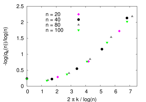
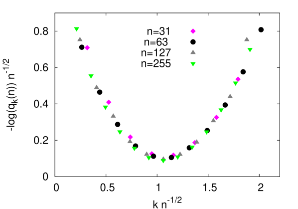
Figure 8: Left : Plot of $-\log(q_{k}(n)/\log{n})$ as a function of $2\pi k/\log{n}$ for Kac polynomials (3) with $d=2$ and for different values of $n=20,40,80$ and $100$. Right : Plot of $-\log{(q_{k}(n))}n^{-1/2}$ as a function of $k/\sqrt{n}$ for binomial polynomials (7) for different values of $n=31,63,127$ and $255$.

III.4 Distribution of the maximum of real roots

Up to now, we have mainly focused on the distribution of the minimum $\lambda_{\rm min}$ of the absolute values $\{|\lambda_{i}|\}$ of the real roots of these polynomials. Indeed, the gap probability $P_{0}([-x,x],n)$ is just the probability that $\lambda_{\rm min}$ is larger than $x>0$. We now instead focus on the distribution of the maximum $\lambda_{\rm max}$ of the $\{|\lambda_{i}|\}$.

III.4.1 Mean Field approximation

As a first approach, we consider the Mean Field or Poissonian approximation introduced above, where one neglects the correlations between the real roots. Then, for any random polynomial ${Q}_{n}(x)=\sum_{i=0}^{n}b_{i}x^{i}$, the probability that $\lambda_{\rm max}\leq x$ is simply the probability that ${Q}_{n}(x)$ has no real root in $[-\infty,-x]\cup[x,+\infty]$. Therefore, within the Mean Field approximation one has

$${\rm Proba.}\;(\lambda_{\rm max}\leq x,n)=\exp{\left(-2\int_{x}^{\infty}\rho_{n}(t)dt\right)}\;.$$ (109)

Taking the derivative of this expression (109) with respect to $x$, one obtains the probability distribution function (pdf) $p_{{\rm max}}(x,n)$ of the maximum $\lambda_{\rm max}$ as

$$p_{{\rm max}}(x,n)=2\rho_{n}(x)\exp{\left(-2\int_{x}^{\infty}\rho_{n}(t)dt\right)}\;.$$ (110)

To obtain the large $x$ behavior of $p_{{\rm max}}(x,n)$ one computes the one of $\rho_{n}(x)$ whose expression is given by

$$\rho_{n}(x)=\frac{\sqrt{c_{n}(x)(c_{n}^{\prime}(x)/x+c_{n}^{\prime\prime}(x))-[c_{n}^{\prime}(x)]^{2}}}{2\pi c_{n}(x)}\;,\;c_{n}(x)=\sum_{i=0}^{n}\langle b_{i}^{2}\rangle\,x^{2i}\;.$$ (111)

For large $x$, one has $c_{n}(x)=x^{2n}\langle b_{n}^{2}\rangle+x^{2n-2}\langle b_{n-1}^{2}\rangle+{\cal O}(x^{2n-4})$ which gives $\rho_{n}(x)\sim\sqrt{{\langle b_{n-1}^{2}\rangle}/{\langle b_{n}^{2}\rangle}}/(\pi x^{2})$. Finally, from Eq. (110), one obtains for $x\gg 1$

$$p_{{\rm max}}(x,n)\sim 2\rho_{n}(x)\sim\frac{2}{\pi x^{2}}\sqrt{\frac{\langle b_{n-1}^{2}\rangle}{\langle b_{n}^{2}\rangle}}\;.$$ (112)

III.4.2 Exact result for the tail

In fact, the tail of the distribution can be computed exactly by noting that

$${\rm Proba.}(\lambda_{\rm max}\leq x,n)=\overline{P}_{0}\left(\left[-\frac{1}{x},\frac{1}{x}\right],n\right)\,,$$ (113)

where $\overline{P}_{0}([a,b],n)$ is the gap probability associated to the polynomial $\overline{Q}_{n}(x)$ defined such that ${Q}_{n}(x)=x^{n}\overline{Q}_{n}(1/x)$. Similarly, we denote $\overline{\rho}_{n}(x)$ the mean density of real root associated to $\overline{Q}_{n}(x)$. From this exact identity (113), valid for all polynomials ${Q}_{n}(x)$ and all $n\geq 1$, one obtains the asymptotic behavior

$${\rm Proba.}(\lambda_{\rm max}\leq x,n)=1-2\frac{\overline{\rho}_{n}(0)}{x}+{o(x^{-1})}\,,$$ (114)

where we have simply used the definition of $\overline{\rho}_{n}(0)$, provided it is well defined, which is the case for Gaussian random polynomials. From this asymptotic behavior (114), one obtains the pdf $p_{{\rm max}}(x,n)$ of the maximum $\lambda_{\rm max}$ for large $x>0$ as

$$p_{{\rm max}}(x,n)\sim 2\frac{\overline{\rho}_{n}(0)}{x^{2}}\;,\;\overline{\rho}_{n}(0)=\frac{1}{\pi}\sqrt{\frac{\langle b_{n-1}^{2}\rangle}{\langle b_{n}^{2}\rangle}}$$ (115)

where we have used the formula (111) to compute $\overline{\rho}_{n}(0)$. For the various polynomials under consideration here, one thus obtains such a power law tail (115) with $\overline{\rho}_{n}(0)=\pi^{-1}((n-1)/n)^{\tfrac{d-2}{4}}$ for Kac polynomials, $\overline{\rho}_{n}(0)=\sqrt{n}/\pi$ for Weyl polynomials and binomial polynomials. This result shows in particular that the mean value of $\lambda_{\rm max}$ is not defined for these polynomials.

It is interesting to note that the Mean Field approximation (112) gives the exact result for this algebraic tail (115). This might be understood by noting that, apart from a short range repulsion, the real roots of these polynomials are actually weakly correlated. For instance, for Weyl polynomials, we show in Appendix D, see Eq. (162), that the two-point (connected) correlation function of the real roots inside the interval $[-\sqrt{n},\sqrt{n}]$ decays faster than exponentially at large distance (see also Ref. bleher for similar properties of $K_{n}(x)$ and $B_{n}(x)$). On the other hand, the marginal distribution of a single real root is nothing else but $\rho_{n}(x)/\langle N_{n}[-\infty,\infty]\rangle$ which decays algebraically $\rho_{n}(x)\sim 1/x^{2}$ for large $x$. Given that these real roots are weakly correlated, we expect that the distribution of the maximum of these real roots is given by a Fréchet distribution, which indeed has a power law tail, as we found here (115).

III.4.3 Numerical results

We have checked numerically this exact asymptotic behavior (115) for the three classes of random polynomials (3, 6, 7). In all the three cases the pdf of the maximum $\lambda_{\rm max}$ was obtained by averaging over $10^{5}$ different realizations of the random Gaussian variables $a_{i}$’s. In the left panel of Fig. 9, we show a plot of $p_{{\rm max}}(x,n)$ as a function of $x$ for Kac polynomials and $d=2$, for different values of $n=8,16$ and $32$. Notice that the exact result in Eq. (115), which is plotted here with a dotted line, is in principle true for all $n\geq 1$ so that it is not necessary to perform numerics for polynomials of large degree. This figure shows a good agreement between our analytic result and the numerics. Similarly, in the right panel of Fig. 9, we have plotted $p_{{\rm max}}(x,n)/\sqrt{n}$ for Weyl polynomials $W_{n}(x)$ and for different values of $n=8,16$ and $32$. Here again, the agreement with the analytical result in Eq. (115) is quite good.

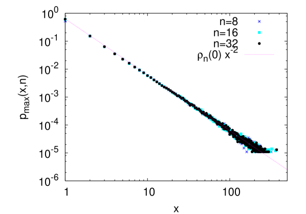
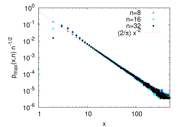
Figure 9: Left : $p_{{\rm max}}(x,n)$ for Kac polynomials $K_{n}(x)$ (3) and $d=2$ as a function of $x$ for different values of $n=8,16$ and $32$. The dotted line is the exact result for the tail of the distribution (115). Right : $p_{{\rm max}}(x,n)/\sqrt{n}$ for Weyl polynomials $W_{n}(x)$ (6) as a function of $x$ for different values of $n=8,16$ and $32$. The dotted line is the exact result for the tail of the distribution (115)

IV Conclusions and perspectives

In conclusion, we have investigated different statistical properties of the real roots of three different types of real random polynomials (3, 6, 7). In these three classes, the mean density of real roots exhibit a rich variety of behaviors, as shown in Figs 1-3. We have first focused on gap probabilities (56, 91, 95) which were shown to be closely related to the persistence probability for the diffusion equation with random initial conditions in dimension $d$ (1, 2). We proposed a Mean Field approximation to compute the exponents as well as the universal scaling functions describing these gap probabilities. Furthermore, we showed how to improve systematically this MF approximation (see Fig. 4, 6) using an $\epsilon$-expansion based on the so called persistence with partial survival. In the case of binomial polynomials $B_{n}(x)$ (7), this allows to obtain exact results for the gap probability (94). Our main results for the gap probability $q_{0}(n)$ on the full real axis are summarized in Fig. 10. We hope that these connections may help to obtain exact results for the exponent $\theta(d)$, which remains a challenge.

Figure 10: Summary of the main results for the probability of no root on the full real axis $q_{0}(n)$ for the three different classes of polynomials $K_{n}(x),W_{n}(x)$ and $B_{n}(x)$.

Besides, we extended our analysis to the probability that these random polynomials have exactly $k$ real roots in a given interval $[a,b]$. We have shown, in the three cases, that this probability has an interesting scaling form characterized by a large deviation function (100-102). We proposed a Mean Field approximation which reproduces qualitatively these scaling forms, which were further checked numerically (see Fig. 8). A similar question was asked in the past for Ginibre real matrices : what is the probability that such $n\times n$ matrices has exactly $k$ real roots ? Quite recently, in Ref. kanzieper_akemann , Akemann and Kanzieper obtained an exact formula for this probability. In that case, the mean number of real roots grows like $\sqrt{n}$ and our MF approximation would therefore suggest a scaling form for this probability similar to Eq. (101). It would be very interesting to extract the large deviation function from an asymptotic analysis of the exact result of Ref. kanzieper_akemann .

Finally, we computed the pdf of the largest real root of these random polynomials. We showed that for a wide class of random polynomials, this pdf has an algebraic tail with exponent $-2$ as shown in Eq. (115) and it would certainly be interesting to extend these results to the case of non-Gaussian random polynomials.

Appendix A Calculation of the mean density for generalized Kac’s polynomials

In this appendix, we give some details concerning the computation of the mean density and the mean number of real roots for Kac’s polynomials $K_{n}(x)$ (3).

A.1 Scaling form

The starting point of the calculation is the formula for the density $\rho_{n}(x)$ given in Eq. (21), which using Eq. (15) gives

$$\rho_{n}(x)=\frac{1}{\pi}\sqrt{\frac{s_{d/2+1,n}(x)}{1+x^{2}s_{d/2-1,n}(x)}-\left(\frac{s_{d/2,n}(x)}{1+s_{d/2-1}(x)}\right)^{2}}\;,$$ (116)

$$\text{with}\quad s_{k,n}(x)=\sum_{i=1}^{n}i^{k}x^{2i-2}\;.$$

In the limit $n\gg 1$, and $|1-x|\ll 1$ keeping $y=n(1-x)$ fixed, $s_{k,n}(x)$ can be viewed as a Riemann sum, thus

$$s_{k,n}(x)\sim n^{k+1}\int_{0}^{1}dxx^{k}e^{-2ux}\quad,\quad u=n(1-x)\;.$$ (117)

Finally using Eq. (117) together with Eq. (116) yield the formula (28) given in the text :

$$\rho_{n}(x)=n\rho^{K}(n(1-x))\;,\;\rho^{K}(y)=\frac{1}{\pi}\sqrt{\frac{I_{d/2+1}(y)}{I_{d/2-1}(y)}-\left(\frac{I_{d/2}(y)}{I_{d/2-1}(y)}\right)^{2}}\;,$$ (118)

$$I_{m}(y)=\int_{0}^{1}dx\;x^{m}\exp{(-2yx)}\;.$$ (119)

A.2 Asymptotic expansions

To compute the asymptotic behaviors of the function $\rho^{K}(y)$ in Eq. (28), one needs the asymptotic behaviors of $I_{m}(y)$ defined above (119).

A.2.1 The limit $y\to\infty$

In that limit, one writes $I_{m}(y)$ as

$$I_{m}(y) = y^{-1-m}\int_{0}^{y}duu^{m}e^{-2u}=y^{-1-m}\int_{0}^{\infty}duu^{m}e^{-2u}+{\cal O}(y^{m}e^{-2y})$$ (120)

$$= (2y)^{-1-m}\Gamma(1+m)+{\cal O}(y^{m}e^{-2y})\;,$$

which, together with Eq. (28), gives the first line of the formula given in Eq. (30) in the text.

A.2.2 The limit $y\to-\infty$

Because of several cancellations occurring in $\rho^{K}(y)$ in the limit $y\to-\infty$ one needs the three first terms in the asymptotic behavior of $I_{m}(y)$ in that limit :

$$I_{m}(y) = |u|^{-1-m}\int_{0}^{|y|}du\;u^{m}e^{2u}$$ (121)

$$= e^{2|y|}\left(\frac{1}{2|y|}-\frac{m}{4y^{2}}+\frac{m(m-1)}{8|y|^{3}}+{\cal O}(y^{-4})\right)\;,$$

which after a tedious but straightforward calculations, using Eq. (28), gives the second line of the formula given in Eq. (30) in the text.

Appendix B Calculation of the mean density for real Weyl’s polynomials

In this section, we present the details of the calculation leading to the scaling form given in Eq. (43). We start with the expression for the mean density given in Eq. (41) with $x=u\sqrt{n}$:

$$\rho_{n}(x)=\rho_{n}(\sqrt{n}u)=\frac{1}{\pi}\sqrt{1+\frac{n^{n+1}u^{2n}(u^{2}-1-n^{-1})}{e^{nu^{2}}\Gamma(n+1,nu^{2})}-\frac{n^{2n+1}u^{4n+2}}{(e^{nu^{2}}\Gamma(n+1,nu^{2}))^{2}}}\;.$$ (122)

We want to obtain the limit $n\to\infty$, keeping $u$ fixed, in the above equation (122) . For that purpose, we need the large $n$ behavior of $\Gamma(n,nu^{2})$ for large $n$ and $u$ fixed. One writes

$$\Gamma(n,nu^{2})=n^{n}\int_{u^{2}}^{\infty}\frac{dx}{x}\;e^{-n(x-\log{x})}=n^{n}\int_{\log{u^{2}}}^{\infty}dy\;e^{-nf(y)}\quad,\quad f(y)=y-\log{y}\;,$$ (123)

and under this form (123) we can now perform a saddle-point calculation. The function $f(y)$ has a single minimum at $y=1$ and therefore we expect that the large $n$ behavior of the expression in Eq. (123) will depend on the sign of $u-1$. For $u<1$ the minimum of $f(y)$ lies in the interval of integration in Eq. (123) and one gets a result independent of $u$

$$\Gamma(n+1,nu^{2})=\sqrt{2\pi}n^{n+1/2}e^{-n}\left(1+{\cal O}(n^{-1/2})\right)\quad,\quad u<1\;.$$ (124)

On the other hand, for $u>1$ the minimum of $f(y)$ in Eq. (123) lies outside the interval of integration and one gets instead

$$\Gamma(n+1,nu^{2})=n^{n-1}e^{-nu^{2}}\frac{u^{2n}}{u^{2}-1}\left(1-\frac{1}{n}\frac{u^{2}}{(u^{2}-1)^{2}}+{\cal O}(n^{-2})\right)\quad,\quad u>1\;.$$ (125)

Using the asymptotic expansion for $u<1$ (124) together with Eq. (122) one obtains straightforwardly that for $u<1$ fixed and large $n$

$$\rho_{n}(\sqrt{n}u)=\frac{1}{\pi}+{\cal O}(n^{-1/2})\quad,\quad u<1\;,$$ (126)

yielding, in the limit $n\to\infty$ the expression (43) given in the text. Similarly, using Eq. (125) together with Eq. (122), one gets for $u>1$ fixed and large $n$

$$\rho_{n}(\sqrt{n}u)={\cal O}(n^{-1})\quad,\quad u>1\;,$$ (127)

yielding, in the limit $n\to\infty$ the expression (43) given in the text.

Appendix C Computation of $\langle N^{2}_{n}([0,x])\rangle_{c}$ for Kac’s polynomials and $d=2$

C.1 Scaling form

In this appendix, we give the details of the computation of $\langle N^{2}_{n}([0,x])\rangle$ which lead to formula (80) given in the text. We start from the general formula valid for all $n$ bendat (see also bleher )

$$\langle N^{2}_{n}([0,x])\rangle=\int_{0}^{x}dt\rho_{n}(t)+\int_{0}^{x}dt_{1}\int_{0}^{x}dt_{2}{\cal K}_{n,2}(t_{1},t_{2})\;,$$ (128)

where ${\cal K}_{n,2}(t_{1},t_{2})$ is the $2$-point correlation function of real roots of $K_{n}(x)$, given by

$${\cal K}_{n,2}(t_{1},t_{2})=\frac{1}{4\pi^{2}\sqrt{\det\Delta_{n}(t_{1},t_{2})}}\int_{-\infty}^{\infty}\int_{-\infty}^{\infty}|y_{1}y_{2}|e^{-\tfrac{1}{2}(Y\Omega_{n}(t_{1},t_{2}),Y)}dy_{1}dy_{2}\;,$$ (129)

where $Y=(y_{1},y_{2})$, $\Delta_{n}(t_{1},t_{2})$ is the $4\times 4$ covariance matrix of $(K_{n}(t_{1}),K_{n}^{\prime}(t_{1}),K_{n}(t_{2}),K^{\prime}_{n}(t_{2}))$ and $\Omega_{n}(t_{1},t_{2})$ is the $2\times 2$ matrix obtained by removing the first and the third rows and columns from $\Delta_{n}(t_{1},t_{2})^{-1}$. In the limit $0<1-t_{1}\ll 1$, $0<1-t_{2}\ll 1$ and $n\to\infty$, keeping $u_{1}=n(1-t_{1})$, $u_{2}=n(1-t_{2})$ fixed one has

$$\langle K_{n}(t_{1})K_{n}(t_{2})\rangle=ng(u_{1}+u_{2})\;,\;g(x)=\frac{1-e^{-x}}{x}\;,$$

$$\langle K_{n}(t_{1})K^{\prime}_{n}(t_{2})\rangle=\langle K^{\prime}_{n}(t_{1})K_{n}(t_{2})\rangle=-n^{2}g^{\prime}(u_{1}+u_{2})\;,$$

$$\langle K^{\prime}_{n}(t_{1})K^{\prime}_{n}(t_{2})\rangle=n^{3}g^{\prime\prime}(u_{1}+u_{2})\;.$$ (130)

Using these relations (130), one obtains the matrix $\Delta_{n}(t_{1},t_{2})$ in this scaling limit as

$$\Delta_{n}(t_{1},t_{2})=\begin{pmatrix}n\,g(2u_{1})&-n^{2}\,g^{\prime}(2u_{1})&n\,g(u_{1}+u_{2})&-n^{2}\,g^{\prime}(u_{1}+u_{2})\\ -n^{2}\,g^{\prime}(2u_{1})&n^{3}\,g^{\prime\prime}(2u_{1})&-n^{2}\,g^{\prime}(u_{1}+u_{2})&n^{3}\,g^{\prime\prime}(u_{1}+u_{2})\\ n\,g(u_{1}+u_{2}&-n^{2}\,g^{\prime}(u_{1}+u_{2})&n\,g(2u_{2})&-n^{2}\,g^{\prime}(2u_{2})\\ -n^{2}\,g^{\prime}(u_{1}+u_{2})&n^{3}\,g^{\prime\prime}(u_{1}+u_{2})&-n^{2}\,g^{\prime}(2u_{2})&n^{3}\,g^{\prime\prime}(2u_{2})\end{pmatrix}\;,$$ (131)

from which one gets

$$\det\Delta_{n}(t_{1},t_{2})=n^{8}\det\tilde{\Delta}(u_{1},u_{2})\;,$$ (132)

$$\tilde{\Delta}(u_{1},u_{2})=\begin{pmatrix}g(2u_{1})&-g^{\prime}(2u_{1})&g(u_{1}+u_{2})&-g^{\prime}(u_{1}+u_{2})\\ -g^{\prime}(2u_{1})&g^{\prime\prime}(2u_{1})&-g^{\prime}(u_{1}+u_{2})&g^{\prime\prime}(u_{1}+u_{2})\\ g(u_{1}+u_{2}&-g^{\prime}(u_{1}+u_{2})&g(2u_{2})&-g^{\prime}(2u_{2})\\ -g^{\prime}(u_{1}+u_{2})&g^{\prime\prime}(u_{1}+u_{2})&-g^{\prime}(2u_{2})&g^{\prime\prime}(2u_{2})\end{pmatrix}\;.$$ (133)

From the structure of $\Delta_{n}(t_{1},t_{2})$ in the scaling limit (131), one obtains the one of $\Omega_{n}(t_{1},t_{2})$ in Eq. (129) as

$$\Omega_{n}(t_{1},t_{2})=n^{-3}\tilde{\Omega}(u_{1},u_{2})\;,$$ (134)

$$\tilde{\Omega}(u_{1},u_{2})=\begin{pmatrix}A(u_{1},u_{2})&B(u_{1},u_{2})\\ B(u_{1},u_{2})&C(u_{1},u_{2})\end{pmatrix}\;,$$ (135)

where $\tilde{\Omega}(u_{1},u_{2})$, is obtained by removing the first and the third rows and columns from $\tilde{\Delta}(u_{1},u_{2})^{-1}$. The functions $A(u_{1},u_{2}),B(u_{1},u_{2}),C(u_{1},u_{2})$ have complicated expressions not given here which can be easily computed e.g. using Mathematica. Using the scaling forms (132, 134) one obtains ${\cal K}_{n,2}(t_{1},t_{2})$ in Eq. (129) in the scaling limit as

$${\cal K}_{n,2}(t_{1},t_{2})=n^{2}\tilde{\cal K}(u_{1},u_{2})$$ (136)

$$\tilde{\cal K}=\frac{(\det\tilde{\Delta})^{-{1}/{2}}}{\pi^{2}AC(1-(\delta)^{2})}\left(1+\frac{\delta}{\sqrt{1-(\delta)^{2}}}\operatorname{ArcSin}\delta\right)\;,\;\delta=\frac{B}{\sqrt{A\,C}}\;.$$ (137)

where we used the notation $\tilde{\Delta}\equiv\tilde{\Delta}(u_{1},u_{2})$ and the expression bleher (see also Ref. bendat )

$$\int_{-\infty}^{\infty}\int_{-\infty}^{\infty}|y_{1}y_{2}|e^{-\tfrac{1}{2}(Ay_{1}^{2}+2By_{1}y_{2}+Cy_{2}^{2})}dy_{1}dy_{2}=\frac{4}{AC(1-(\delta)^{2})}\left(1+\frac{\delta}{\sqrt{1-(\delta)^{2}}}\operatorname{ArcSin}\delta\right)$$ (138)

Using this scaling form (136), together with the one for the density in Eq. (28), one obtains $\langle N_{n}([0,x])^{2}\rangle_{c}$ in the limit $0<(1-x)\ll 1$, with $n\to\infty$ keeping $y=n(1-x)$ fixed as

$$\langle N_{n}([0,x])^{2}\rangle_{c}\sim\int_{y}^{n}\rho^{K}(u)du+\int_{y}^{n}du_{1}\int_{y}^{n}du_{2}\,(\tilde{\cal K}(u_{1},u_{2})-\rho^{K}(u_{1})\rho^{K}(u_{2}))\;.$$ (139)

Alternatively, one can write Eq. (139) in the large $n$ limit as

$$\langle N_{n}([0,x])^{2}\rangle-\langle N_{n}([0,1])^{2}\rangle=-\nu_{-}(n(1-x))$$ (140)

$$\nu_{-}(y)=\int_{0}^{y}du\rho^{K}(u)+2\int_{0}^{y}du_{1}\int_{u_{1}}^{\infty}du_{2}\,(\tilde{\cal K}(u_{1},u_{2})-\rho^{K}(u_{1})\rho^{K}(u_{2}))\;.$$ (141)

C.2 Large argument behavior of $\nu_{-}(y)$

To compute $\nu_{-}(y)$ in the large $y$ limit, one compute $d{\nu_{-}}(y)/dy$ from Eq. (141)

$$\frac{d\nu_{-}(y)}{dy}=\rho^{K}(y)+2\int_{y}^{\infty}du_{2}(\tilde{\cal K}(y,u_{2})-\rho^{K}(y)\rho^{K}(u_{2}))\;.$$ (142)

The large $y$ behavior of $\rho^{K}(y)$ has been computed previously (30). To extract the large $y$ behavior of $d{\nu_{-}}(y)/dy$, one thus needs to compute the behavior of $\tilde{\cal K}(u_{1},u_{2})$ for $u_{1},u_{2}\gg 1$. We first analyse the behavior $\tilde{\Delta}(u_{1},u_{2})$ in Eq. (133) for $u_{1},u_{2}\gg 1$. This yields

$$\tilde{\Delta}(u_{1},u_{2})\sim\begin{pmatrix}\frac{1}{2u_{1}}&\frac{1}{4u_{1}^{2}}&\frac{1}{u_{1}+u_{2}}&\frac{1}{(u_{1}+u_{2})^{2}}\\ \frac{1}{4u_{1}^{2}}&\frac{1}{4u_{1}^{3}}&\frac{1}{(u_{1}+u_{2})^{2}}&\frac{2}{(u_{1}+u_{2})^{3}}\\ \frac{1}{u_{1}+u_{2}}&\frac{1}{(u_{1}+u_{2})^{2}}&\frac{1}{2u_{2}}&\frac{1}{4u_{2}^{2}}\\ \frac{1}{(u_{1}+u_{2})^{2}}&\frac{2}{(u_{1}+u_{2})^{3}}&\frac{1}{4u_{2}^{2}}&\frac{1}{4u_{2}^{3}}\end{pmatrix}\;,$$ (143)

from which one gets

$$\det\tilde{\Delta}(u_{1},u_{2})\sim\frac{1}{256(u_{1}u_{2})^{4}}\left(\frac{u_{1}-u_{2}}{u_{1}+u_{2}}\right)^{8}\;.$$ (144)

From Eq. (143), one gets the behavior of the matrix $\tilde{\Omega}$ in Eq. (135) as

$$A(u_{1},u_{2})\sim 8u_{1}^{3}\left(\frac{u_{1}+u_{2}}{u_{1}-u_{2}}\right)^{4}$$ (145)

$$B(u_{1},u_{2})\sim 16\frac{u_{1}^{2}u_{2}^{2}}{u_{1}+u_{2}}\left(\frac{u_{1}+u_{2}}{u_{1}-u_{2}}\right)^{4}$$ (146)

$$C(u_{1},u_{2})\sim 8u_{2}^{3}\left(\frac{u_{1}+u_{2}}{u_{1}-u_{2}}\right)^{4}$$ (147)

which gives $\delta=B/\sqrt{AC}$ as

$$\delta(u_{1},u_{2})\sim\frac{2\sqrt{u_{1}u_{2}}}{u_{1}+u_{2}}$$ (148)

Finally, using Eq. (145-148) together with Eq. (30) in $d=2$ one gets

$$\tilde{\cal K}(u_{1},u_{2})-\rho^{K}(u_{1})\rho^{K}(u_{2})\sim-\frac{1}{\pi^{2}(u_{1}+u_{2})^{2}}+\frac{1}{2\pi^{2}\sqrt{u_{1}u_{2}}}\frac{|u_{1}-u_{2}|}{(u_{1}+u_{2})^{2}}\operatorname{ArcSin}{\frac{2\sqrt{u_{1}u_{2}}}{u_{1}+u_{2}}}\;.$$ (149)

Therefore, from Eq. (142), one gets

$$\frac{d\nu_{-}(y)}{dy}\sim\frac{1}{y}\left(\frac{2}{\pi^{2}}-\frac{1}{\pi}\right)+{\cal O}(y^{-2})\;,$$ (150)

where we have used the identity

$$\int_{1}^{\infty}\frac{dv}{\sqrt{v}}\frac{v-1}{(v+1)^{2}}\operatorname{ArcSin}\left(\frac{2\sqrt{v}}{v+1}\right)=\frac{\pi}{2}-1\;.$$ (151)

Finally, one gets from Eq. (150) that

$$\nu_{-}(y)\sim\left(\frac{2}{\pi^{2}}-\frac{1}{\pi}\right)\log{y}+{\cal O}(1)\;.$$ (152)

Appendix D Computation of $\langle N^{2}_{n}([-x,x])\rangle_{c}$ for Weyl polynomials

D.1 Scaling form

In this appendix we give the detail of the computation of $\langle N_{n}([-x,x])^{2}\rangle$ which leads to formula (86) in the text. Here again we start from the general formula valid for all $n$, similarly to Eq. (128)

$$\langle N^{2}_{n}([-x,x])\rangle=\int_{-x}^{x}dt\rho_{n}(t)+\int_{-x}^{x}dt_{1}\int_{-x}^{x}dt_{2}{\cal W}_{n,2}(t_{1},t_{2})\;,$$ (153)

where ${\cal W}_{n,2}(t_{1},t_{2})$ is the $2$-point correlation function of the real roots of $W_{n}(x)$, given by formula (129) where $K_{n}(x)$ is replaced by $W_{n}(x)$:

$${\cal W}_{n,2}(t_{1},t_{2})=\frac{1}{4\pi^{2}\sqrt{\det\Delta_{n}(t_{1},t_{2})}}\int_{-\infty}^{\infty}\int_{-\infty}^{\infty}|y_{1}y_{2}|e^{-\tfrac{1}{2}(Y\Omega_{n}(t_{1},t_{2}),Y)}dy_{1}dy_{2}\;,$$ (154)

where $Y=(y_{1},y_{2})$, $\Delta_{n}(t_{1},t_{2})$ is the $4\times 4$ covariance matrix of $(W_{n}(t_{1}),W_{n}^{\prime}(t_{1}),W_{n}(t_{2}),W^{\prime}_{n}(t_{2}))$ and $\Omega_{n}(t_{1},t_{2})$ is the $2\times 2$ matrix obtained by removing the first and the third rows and columns from $\Delta_{n}(t_{1},t_{2})^{-1}$. In the limit $n\to\infty$, keeping $t_{1}<\sqrt{n}$, $t_{2}<\sqrt{n}$ fixed one has

$$\langle W_{n}(t_{1})W_{n}(t_{2})\rangle=e^{t_{1}t_{2}}\;,$$

$$\langle W^{\prime}_{n}(t_{1})W_{n}(t_{2})\rangle=t_{2}e^{t_{1}t_{2}}\;,$$

$$\langle W_{n}(t_{1})W^{\prime}_{n}(t_{2})\rangle=t_{1}e^{t_{1}t_{2}}\;,$$

$$\langle W^{\prime}_{n}(t_{1})W^{\prime}_{n}(t_{2})\rangle=(1+t_{1}t_{2})e^{t_{1}t_{2}}\;,$$ (155)

from which we obtain $\Delta_{n}(t_{1},t_{2})=\tilde{\Delta}(t_{1},t_{2})$ as

$$\tilde{\Delta}(t_{1},t_{2})=\begin{pmatrix}e^{t_{1}^{2}}&t_{1}e^{t_{1}^{2}}&e^{t_{1}t_{2}}&t_{1}e^{t_{1}t_{2}}\\ t_{1}e^{t_{1}^{2}}&(1+t_{1}^{2})e^{t_{1}^{2}}&t_{2}e^{t_{1}t_{2}}&(1+t_{1}t_{2})e^{t_{1}t_{2}})\\ e^{t_{1}t_{2}}&t_{2}e^{t_{1}t_{2}}&e^{t_{2}^{2}}&t_{2}e^{t_{2}^{2}}\\ t_{1}e^{t_{1}t_{2}}&(1+t_{1}t_{2})e^{t_{1}t_{2}}&t_{2}e^{t_{2}^{2}}&(1+t_{2}^{2})e^{t_{2}^{2}}\end{pmatrix}\;.$$ (156)

The determinant is easily obtained as

$$\det\tilde{\Delta}(t_{1},t_{2})=e^{(t_{1}+t_{2})^{2}}\left(4\sinh^{2}{\left(\frac{(t_{1}-t_{2})^{2}}{2}\right)}-(t_{1}-t_{2})^{4}\right)$$ (157)

From $\tilde{\Delta}(t_{1},t_{2})$ in Eq. (156), one obtains $\Omega_{n}(t_{t},t_{2})=\tilde{\Omega}(t_{1},t_{2})$ for large $n$ as

$$\tilde{\Omega}(t_{1},t_{2})=\begin{pmatrix}D(t_{1},t_{2}&E(t_{1},t_{2}))\\ E(t_{2},t_{2})&F(t_{1},t_{2})\end{pmatrix}$$ (158)

with

$$D(t_{1},t_{2})=\frac{e^{t_{1}^{2}+2t_{2}^{2}}}{\tilde{\Delta}(t_{1},t_{2})}(1-e^{-(t_{1}-t_{2})^{2}}(1+(t_{1}-t_{2})^{2}))\;,$$

$$E(t_{1},t_{2})=\frac{e^{3t_{1}t_{2}}}{\tilde{\Delta}(t_{1},t_{2})}(1-e^{(t_{1}-t_{2})^{2}}(1-(t_{1}-t_{2})^{2}))\;,$$

$$F(t_{1},t_{2})=\frac{e^{2t_{1}^{2}+t_{2}^{2}}}{\tilde{\Delta}(t_{1},t_{2})}(1-e^{-(t_{1}-t_{2})^{2}}(1+(t_{1}-t_{2})^{2}))\;.$$ (159)

Finally, using these expressions (159) together with the formula in Eq. (138), one obtains from Eq. (154) that ${\cal W}_{n,2}(t_{1},t_{2})=\tilde{\cal W}(t_{1}-t_{2})$ with

$$\tilde{\cal W}(s)=\frac{1}{\pi^{2}}\frac{((1-e^{-s^{2}})^{2}-s^{4}e^{-s^{2}})^{\tfrac{1}{2}}}{1-e^{-s^{2}}}\left(1+\frac{\delta(s)}{\sqrt{1-(\delta(s))^{2}}}\operatorname{ArcSin}\delta(s)\right)\;,$$ (160)

with

$$\delta(s)=\frac{e^{-s^{2}/2}(e^{-s^{2}}+s^{2}-1)}{1-e^{-s^{2}}-s^{2}e^{-s^{2}}}\;.$$ (161)

Notice that $\tilde{\cal W}(s)$ is the two point correlation function of real zeros of $W_{n}(x)$. Interestingly, this correlation function in Eq. (160) coincides (up to a multiplicative prefactor $\pi^{-2}$) with the correlation of straightened zeros of $B_{n}(x)$ obtained in bleher . Its asymptotic behaviors are given by

$$\tilde{\cal W}(s)\sim\begin{cases}\tfrac{|s|}{4\pi}\;,\;s\to 0\\ \tfrac{1}{\pi^{2}}+\tfrac{s^{4}e^{-s^{2}}}{2\pi^{2}}\;,\;s\to\infty\end{cases}$$ (162)

Finally, using the expression (153) together with Eq. (154) one has for $0<x<\sqrt{n}$, in the limit $n\to\infty$

$$\langle N^{2}_{n}([-x,x])\rangle_{c}=\nu(x)\;,$$

$$\nu(x)=\frac{2x}{\pi}+2\int_{0}^{2x}ds(2x-s)(\tilde{\cal W}(s)-\pi^{-2})\;.$$ (163)

D.2 Large argument behavior of $\nu(x)$

To analyse the large $x$ behavior of $\nu(x)$, one computes $d\nu(x)/dx$ and gets immediately

$$\lim_{x\to\infty}\frac{d\nu(x)}{dx}=\frac{2}{\pi}+4\int_{0}^{\infty}ds(\tilde{\cal W}(s)-\pi^{-2})$$ (164)

such that

$$\nu(x)\propto 2\nu_{\infty}x\;,\;x\gg 1$$ (165)

with $\nu_{\infty}=0.181988...$, which leads to the value of $\theta_{\infty}$ up to order ${\cal O}(\epsilon^{2})$ given in Eq. (89).

Appendix E Computation of $\langle N^{3}_{n}([a,b])\rangle_{c}$ for binomial polynomials

In this appendix, we give the detailed calculation of $\langle N^{3}_{n}([a,b])\rangle_{c}$ which leads to the formula (93) given in the text, for $m=3$. We start with the general formula (see for instance Ref. bleher ):

$$\langle N^{3}_{n}([a,b])\rangle_{c}=\langle N_{n}[a,b]\rangle+3\langle N^{2}_{n}[a,b]\rangle_{c}$$ (166)

$$+\int_{a}^{b}dt_{1}\int_{a}^{b}dt_{2}\int_{a}^{b}dt_{3}\left({\cal B}_{n,3}(t_{1},t_{2},t_{3})-3{\cal B}_{n,2}(t_{1},t_{2})\rho_{n}(t_{3})+\rho_{n}(t_{1})\rho_{n}(t_{2})\rho_{n}(t_{3})\right)\;,$$ (167)

where ${\cal B}_{n,m}$ is the $m$-point correlation function of real roots of $B_{n}(x)$. In Eq. (166), ${\cal B}_{n,2}(t_{1},t_{2})$ is given by the formula (129) where $K_{n}(x)$ is replaced by $B_{n}(x)$ and ${\cal B}_{n,3}(t_{1},t_{2},t_{3})$ is formally given by (see for instance Ref. bleher )

$${\cal B}_{n,3}(t_{1},t_{2},t_{3})=\int_{-\infty}^{\infty}dy_{1}\int_{-\infty}^{\infty}dy_{2}\int_{-\infty}^{\infty}dy_{3}|y_{1}y_{2}y_{3}|D_{n,3}(0,y_{1},0,y_{2},0,y_{3};t_{1},t_{2},t_{3})\;,$$ (168)

where $D_{n,3}(x_{1},y_{1},x_{2},y_{2},x_{3},y_{3})$ is the joint distribution density of $(B_{n}(t_{1}),B^{\prime}_{n}(t_{1}),(B_{n}(t_{2}),B^{\prime}_{n}(t_{2}),(B_{n}(t_{3}),B^{\prime}_{n}(t_{3}))$. According to Eq. (92), the two terms in (166) have the desired form (93) for large $n$. To study the triple integral in Eq. (167) in the large $n$ limit, we will use the results obtained in Ref. bleher :

$$\lim_{n\to\infty}\left[\frac{{\cal B}_{n,2}(t_{1},t_{2})}{\rho_{n}(t_{1})\rho_{n}(t_{2})}\right]_{t_{i}=\langle N[0,s_{i}]\rangle^{-1}}=b_{2}(s_{1},s_{2})\equiv b_{2}(s_{1}-s_{2})\;,$$ (169)

where $\langle N[0,s_{i}]\rangle^{-1}$ is the inverse function of $\langle N[0,s_{i}]\rangle$. Similarly

$$\lim_{n\to\infty}\left[\frac{{\cal B}_{n,3}(t_{1},t_{2},t_{3})}{\rho_{n}(t_{1})\rho_{n}(t_{2})\rho_{n}(t_{3})}\right]_{t_{i}=\langle N[0,s_{i}]\rangle^{-1}}=b_{3}(s_{1},s_{2},s_{3})\equiv b_{3}(s_{1}-s_{2},s_{2}-s_{3})\;,$$ (170)

where $b_{2}(u)$ and $b_{3}(u,v)$ are well defined functions, with a quite complicated expression not given here (see Ref. bleher for more detail). Given these results (169, 170), it is natural to perform the change of variable $s_{i}=\langle N_{n}[0,t_{i}]\rangle$ in Eq. (167), which yields

$$\int_{0}^{x}dt_{1}\int_{0}^{x}dt_{2}\int_{0}^{x}dt_{3}\left({\cal B}_{n,3}(t_{1},t_{2},t_{3})-3{\cal B}_{n,2}(t_{1},t_{2})\rho_{n}(t_{3})+\rho_{n}(t_{1})\rho_{n}(t_{2})\rho_{n}(t_{3})\right)$$ (171)

$$=\int_{\langle N_{n}[0,a]\rangle}^{\langle N_{n}[0,b]\rangle}ds_{1}\int_{\langle N_{n}[0,a]\rangle}^{\langle N_{n}[0,b]\rangle}ds_{2}\int_{\langle N_{n}[0,a]\rangle}^{\langle N_{n}[0,b]\rangle}ds_{3}\left(b_{3}(s_{1}-s_{2},s_{2}-s_{3})-3b_{2}(s_{1}-s_{2})+2\right)\;.$$ (172)

Performing the change of variables $s_{i}\to s_{i}-\langle N_{n}[0,a]\rangle$, one has

$$\int_{0}^{x}dt_{1}\int_{0}^{x}dt_{2}\int_{0}^{x}dt_{3}\left({\cal B}_{n,3}(t_{1},t_{2},t_{3})-3{\cal B}_{n,2}(t_{1},t_{2})\rho_{n}(t_{3})+\rho_{n}(t_{1})\rho_{n}(t_{2})\rho_{n}(t_{3})\right)$$ (173)

$$=\int_{0}^{\langle N_{n}[a,b]\rangle}ds_{1}\int_{0}^{\langle N_{n}[a,b]\rangle}ds_{2}\int_{0}^{\langle N_{n}[a,b]\rangle}ds_{3}\left(b_{3}(s_{1}-s_{2},s_{2}-s_{3})-3b_{2}(s_{1}-s_{2})+2\right)\;.$$ (174)

Given that $\langle N_{n}[a,b]\rangle\propto\sqrt{n}$ in the large $n$ limit for $a,b>n^{-1/2}$, one gets the multiple integral in Eq. (173) in the large $n$ limit as

$$\int_{0}^{\langle N_{n}[a,b]\rangle}ds_{1}\int_{0}^{\langle N_{n}[a,b]\rangle}ds_{2}\int_{0}^{\langle N_{n}[a,b]\rangle}ds_{3}\left(b_{3}(s_{1}-s_{2},s_{2}-s_{3})-3b_{2}(s_{1}-s_{2})+2\right)$$

$$\sim\sigma\langle N_{n}[a,b]\rangle\;,$$ (175)

with $\sigma=3\int_{-\infty}^{0}du\int_{-\infty}^{0}dv\left(b_{3}(u,v)-3b_{2}(v)+2\right)$, provided this double integral over $u,v$ is well defined (which we can only assume here given the complicated expression of $b_{3}(u,v)$).

Finally, combining Eq. (166, 167, 92) together with Eq. (175) one obtains that

$$\langle N^{3}_{n}[a,b]\rangle_{c}\propto\beta_{3}\langle N_{n}[a,b]\rangle\;,$$ (176)

with $a_{3}=1+3a_{2}+\sigma$. Notice that the crucial point in the derivation of this relation is the fact that $\langle N_{n}[a,b]\rangle\propto\sqrt{n}$ for any fixed $a,b>n^{-1/2}$. One expects a similar mechanism to hold for higher values of $m$, yielding Eq. (93) in the text.

$$\langle N^{m}_{n}[a,b]\rangle_{c}\propto\beta_{m}\langle N_{n}[a,b]\rangle\;.$$ (177)

References

- (1) S.N. Majumdar, Persistence in nonequilibrium systems, Curr. Sci., 77, 370 (1999).
- (2) M. Marcos-Martin, D. Beysens, J. P. Bouchaud, C. Godrèche, and I. Yekutieli, Self-diffusion and ‘visited’ surface in the droplet condensation problem (breath figures), Physica 214D, 396 (1995).
- (3) W. Y. Tam, R. Zeitak, K. Y. Szeto and J. Stavans, First-passage exponent in two-dimensional soap froth, Phys. Rev. Lett. 78, 1588 (1997).
- (4) D. B. Dougherty, I. Lyubinetsky, E. D. Williams, M. Constantin, C. Dasgupta and S. Das Sarma, Experimental persistence probability for fluctuating steps, Phys. Rev. Lett. 89, 136102 (2002).
- (5) G. P. Wong, R. W. Mair, R. L. Walsworth and D. G. Cory, Measurement of persistence in 1D diffusion, Phys. Rev. Lett. 86, 4156 (2001).
- (6) S. N. Majumdar, C. Sire, A. J. Bray, S. J. Cornell, Phys. Rev. Lett. 77, Nontrivial exponent for simple diffusion, 2867 (1996); B. Derrida, V. Hakim and R. Zeitak, Persistent spins in the linear diffusion approximation of phase ordering and zeros of stationary Gaussian processes, ibid. 2871.
- (7) T. J. Newman and W. Loinaz, Critical dimensions of the diffusion equation, Phys. Rev. Lett. 86, 2712 (2001).
- (8) D. S. Palmer, Properties of random functions, Proc. Camb. Phil. Soc. 52, 672 (1956).
- (9) A. Bloch and G. Pólya, On the roots of certain algebraic equations, Proc. London Math. Soc. (3) 33, 102 (1932).
- (10) A. T. Bharucha-Reid and M. Sambandham, Random Polynomials, Academic Press, New York, 1986.
- (11) K. Farahmand, in Topics in random polynomials, Pitman research notes in mathematics series 393, (Longman, Harlow) (1998).
- (12) A. Edelman and E. Kostlan, How many zeros of random polynomials are real ?, Bull. Amer. Math. Soc. 32, 1 (1995).
- (13) E. Bogomolny, O. Bohigas and P. Leboeuf, Distribution of roots of random polynomials, Phys. Rev. Lett. 68, 2726 (1992); Quantum chaotic dynamics and random polynomials, J. Stat. Phys. 85, 639 (1996).
- (14) G. Schehr and S.N. Majumdar, Statistics of the number of zero crossings: from random polynomials to the diffusion equation, Phys. Rev. Lett. 99, 060603 (2007).
- (15) M. Kac, On the average number of real roots of a random algebraic equation, Bull. Amer. Math. Soc. 49, 314 (1943); Erratum: Bull. Amer. Math. Soc. 49, 938 (1943).
- (16) M. Das, Real zeros of a class od random algebraic polynomials, J. Indian Math. Soc. 36, 53 (1972).
- (17) M. L. Mehta, Random matrices, Academic Press, New York, (1991).
- (18) A. Dembo, B. Poonen, Q.-M. Shao, O. Zeitouni, Random polynomials having few or no real zeros, J. Amer. Math. Soc. 15, 857 (2002).
- (19) Y. Castin, Z. Hadzibabic, S. Stock, J. Dalibard and S. Stringari, Quantized vortices in the ideal Bose gas: a physical realization of random polynomials, Phys. Rev. Lett. 96, 040405 (2006).
- (20) P. Bleher and X. Di, Correlations between zeros of a random polynomial, J. Stat. Phys. 88, 269 (1997).
- (21) S. N. Majumdar and A. J. Bray, Persistence with Partial Survival, Phys. Rev. Lett. 81, 2626 (1998).
- (22) D. Slepian, The one-sided barrier problem for Gaussian noise, Bell Syst. Tech. J. 41, 463 (1962).
- (23) J.A. McFadden, The axis-crossing intervals of random functions – II, IRE Trans. Inform. Theor IT-4, 14 (1957).
- (24) H.J. Hilhorst, Persistence exponent of the diffusion equation in epsilon dimensions, Physica A, 277, 124 (2000).
- (25) G. C. M. A. Ehrhardt and A. J. Bray, Series expansion calculation of persistence exponents, Phys. Rev. Lett 88, 070601 (2002).
- (26) S.O. Rice, Mathematical analysis of random noise, Bell Syst. Tech. J., 23, 282 (1944).
- (27) I. S Gradshteyn and I. M. Ryzhik, Tables of integrals, series and products, Academic Press (1980).
- (28) A.P. Aldous and Y.V. Fyodorov, Real roots of random polynomials: universality close to accumulation points, J. Phys. A: Math. Gen. 37, 1231 (2004).
- (29) J.E. Wilkins, An asymptotic expansion for the expected number of real zeros of a random polynomial, Proc. Am. Math. Soc. 42, 1249 (1988).
- (30) A. Edelman, E. Kostlan and M. Schub, How many eigenvalues of a random matrix are real ?, J. Amer. Math. Soc. 7, 247 (1994).
- (31) P. Leboeuf, Random Analytic Chaotic Eigenstates, J. Stat. Phys. 95, 651 (1999).
- (32) N.B. Maslova, On the distribution of the number of real roots of random polynomials, Theor. Proba. Appl. 19, 461 (1974).
- (33) T. W. Burkhardt, Dynamics of inelastic collapse, Phys. Rev. E 63, 011111 (2001).
- (34) G. De Smedt, C. Godrèche, J.M. Luck, Partial survival and inelastic collapse for a randomly accelerated particle, Europhys. Lett. 53, 438 (2001).
- (35) Y.G. Sinai, Distribution of some functionals of the integral of a random walk, Theor. Math. Phys. 90, 219 (1992).
- (36) T.W. Burkhardt, Semiflexible polymer in the half plane and statistics of the integral of a Brownian curve, J. Phys. A : Math. Gen. 26, L1157 (1993).
- (37) E. Kanzieper and G. Akemann, Statistics of real eigenvalues in Ginibre’s ensemble of random real matrices, Phys. Rev. Lett. 95, 230201 (2005); G. Akemann and E. Kanzieper, Integrable structure of Ginibre’s ensemble of real random matrices and a Pfaffian integration theorem, J. Stat. Phys. 129 1159 (2007).
- (38) J.S. Bendat, Principles and Applications of Random Noise Theory, Wiley, New York, (1958).