Quantum Metrology Subject to Instrumentation Constraints

Abstract

Maximizing the precision in estimating parameters in a quantum system subject to instrumentation constraints is cast as a convex optimization problem. We account for prior knowledge about the parameter range by developing a worst-case and average case objective for optimizing the precision. Focusing on the single parameter case, we show that the optimization problems are linear programs. For the average case the solution to the linear program can be expressed analytically and involves a simple search: finding the largest element in a list. An example is presented which compares what is possible under constraints against the ideal with no constraints, the Quantum Fisher Information.

I Introduction

The theoretical limit on the accuracy of parameter estimation in quantum metrology applications has been examined in depth, e.g., Holevo:82 ; BraunsteinC:94 ; SarovarM:06 ; GLM:06 ; BFCG:07 ; ShajiC:07 . These studies reveal that special preparation of the instrumentation – the probe – can achieve an asymptotic variance smaller than the Cramér-Rao lower bound Cramer:46 , often referred to as the Quantum Fisher Information, abbreviate here as QFI. In addition, the unique quantum property of entanglement can increase the parameter estimation convergence rate for $N$ identical, independent experiments from the shot-noise limit of $1/\sqrt{N}$ to the Heisenberg limit of $1/N$.

It is reasonable to expect, with or without entanglement, that the QFI will not be obtained with imperfect and limited instrumentation resources, i.e., not all states can be prepared and not all measurement schemes are possible. Under these conditions what exactly is the best that can be done?

In this paper we present an approach which maximizes the parameter estimation accuracy in the presence of limits on instrumentation, The method is based on the convex optimization approach to optimal experiment design as developed in BoydV:04 and as applied to quantum tomography in KosutWR:04 . Incorporating prior knowledge of the parameter range, we develop a worst-case and average case objective for optimizing the precision. Focusing on the single parameter case, we show that the optimization problems are linear programs. For the average case the solution to the linear program can be expressed analytically and involves a simple search, i.e., finding the largest element in a list. This means that an enormous number of combinations of state and sensor configurations can be efficiently evaluated.

II Optimal Experiment Design

Consider a quantum system dependent on an unknown scalar real parameter $\theta$ which is known a priori to be in a set $\Theta=\left\{\,\theta\,\left|\,\theta_{\min}\leq\theta\leq\theta_{\max}\,\right.\right\}$. The parameter $\theta$ is to be estimated using data from repeated independent, identical experiments. In each experiment the system can be put in any one of $k=1,\ldots,{N_{\rm config}}$ configurations. These are the available settings of input states and measurements. Each experiment in configuration $k$ results in one of ${N_{\rm out}}$ outcomes with probability $p_{i|k}(\theta),\ i=1,\ldots,{N_{\rm out}}$. Let $N_{i|k}(\theta)$ denote the number of times outcome $i$ is obtained from $N_{k}$ identical experiments in configuration $k$. Thus, ${\bf E}{N_{i|k}(\theta)}=N_{k}p_{i|k}(\theta),\ \sum_{i=1}^{N_{\rm out}}\ N_{i|k}(\theta)=N_{k}$ where ${\bf E}$ is the expected value operator with respect to the probability distribution $p_{i|k}(\theta)$. Let $N$ denote the total number of experiments and $\lambda_{k}$ the distribution of experiments in configuration $k$. Thus, $\lambda_{k}=N_{k}/N\ \Rightarrow\ \sum_{k=1}^{N_{\rm config}}\ \lambda_{k}={\bf 1}^{T}\lambda=1$. The problem is to select the distribution of experiments per configuration, $\lambda_{k},k=1,\ldots,{N_{\rm config}}$, or equivalently the number of experiments per configuration, $N_{k}$, so as to obtain an estimate of $\theta\in\Theta$ with the best accuracy from $N$ experiments. The “best” attainable estimation accuracy is defined here as the smallest possible Cramér-Rao bound on the estimation variance Cramer:46 .

Specifically, if ${\widehat{\theta}}_{N}$ is an unbiased estimate of $\theta$ from $N$ data, then the estimation error variance satisfies,

$$\begin{array}[]{l}NF(\lambda,\theta)\ {\bf E}{({\widehat{\theta}}_{N}-\theta)^{2}}\geq 1\\ F(\lambda,\theta)=\lambda^{T}g(\theta)=\sum_{k=1}^{N_{\rm config}}\ \lambda_{k}g_{k}(\theta)\\ g_{k}(\theta)=\sum_{{i}=1}^{N_{\rm out}}\ \Big{(}\nabla_{\theta}\ p_{i|k}(\theta)\Big{)}^{2}/p_{i|k}(\theta)\end{array}$$ (1)

To achieve the best accuracy we will select $\lambda$ so as to maximize a measure of the size of the Fisher Information, $F(\lambda,\theta)$. To account for the knowledge that $\theta\in\Theta$ we will consider two experiment design objectives for selecting $\lambda$: average case and worst-case.

$$\begin{array}[]{c}\mbox{\bf Average-Case Experiment Design}\\ \begin{array}[]{ll}\mbox{maximize}&F_{\rm ac}(\lambda)=\lambda^{T}g_{\rm avg}\\ \mbox{subject to}&{\bf 1}^{T}\lambda=1,\ \mbox{$N\lambda$ is a vector of integers}\end{array}\end{array}$$ (2)

with $g_{\rm avg}=\int p(\theta)g(\theta)d\theta$ where $p(\theta)$ is the probability density associated with $\theta\in\Theta$. Although the objective function (average Fisher information) is linear in $\lambda$, the integer constraint on $\lambda$ makes the optimization problem hard. Utilizing the optimal experiment design method presented in (BoydV:04, , §7.5), the integer constraint is relaxed to the linear inequality $\lambda\geq 0$. In addition, suppose we take a finite number of samples from the set $\Theta$, say, $\left\{\,\theta_{r}\,\left|\,r=1,\ldots,{N_{\theta}}\,\right.\right\}$ Then the non-convex integer optimization (2) is approximated by,

$$\begin{array}[]{ll}\mbox{maximize}&F_{\rm ac}(\lambda)=\lambda^{T}g_{\rm avg},\;g_{\rm avg}=\sum_{r}\ p(\theta_{r})g(\theta_{r})\\ \mbox{subject to}&{\bf 1}^{T}\lambda=1,\ \lambda\geq 0\end{array}$$ (3)

This is a convex optimization problem in $\lambda$, in fact, it is a linear program (LP). However, a particular advantage of this formulation (3), is that the solution is given explicitly by,

$$\begin{array}[]{c}\widehat{\lambda}_{k}=\left\{\begin{array}[]{ll}1&k=\arg\max_{k^{\prime}}\ \sum_{r}\ p(\theta_{r})g_{k^{\prime}}(\theta_{r})\\ 0&\mbox{otherwise}\end{array}\right.\end{array}$$ (4)

with the optimal objective $F_{\rm ac}(\widehat{\lambda})=\max_{k}\ \sum_{r}\ p(\theta_{r})g_{k}(\theta_{r})$. It is possible that there is more than one optimal distribution because $\max_{k}$ may not be unique. However, due to limits on numerical precision, it is more likely that there are other choices which give similar results to the optimal objective.

$$\begin{array}[]{c}\mbox{\bf Worst-Case Experiment Design}\\ \begin{array}[]{ll}\mbox{maximize}&F_{\rm wc}(\lambda)=\min_{\theta\in\Theta}\ \lambda^{T}g(\theta)\\ \mbox{subject to}&{\bf 1}^{T}\lambda=1,\ \mbox{$N\lambda$ is a vector of integers}\end{array}\end{array}$$ (5)

As in the average-case, relaxing the integer constraint and approximating the objective function over a set of $\theta$ sampled from the known set $\Theta$ gives the optimization problem:

$$\begin{array}[]{ll}\mbox{maximize}&F_{\rm wc}(\lambda)=\min_{r}\ \lambda^{T}g(\theta_{r})\\ \mbox{subject to}&{\bf 1}^{T}\lambda=1,\ \lambda\geq 0\end{array}$$ (6)

This is also an LP in $\lambda$, but unlike the average-case, there is no explicit solution. However, it can be solved efficiently for a very large number of configurations ${N_{\rm config}}$. A potential advantage of the average-case solution over the worst-case solution is that only a single configuration is required. As we will see in the example to follow, the two distributions can be quite different even though the Fisher information is similar.

The solution to both of the relaxed and approximated problems (3),(6) provide upper and lower bounds to the unknown solution of each with the integer constraint active. Specifically, let $\lambda^{\rm opt}$ denote a solution to either (3) or (6) with the integer constraint. Let $\widehat{\lambda}$ be a solution to the relaxed (LP) versions. From the latter we can determine a nearby solution which satisfies the integer constraint, e.g., set $\lambda^{\rm rnd}={\bf round}(\widehat{\lambda})$. Then, $F_{\rm ac}(\widehat{\lambda})\leq F_{\rm ac}(\lambda^{\rm opt})\leq F_{\rm ac}(\lambda^{\rm rnd})$ and $N_{k}=N\lambda_{k}^{\rm rnd}$ is the number of experiments to repeat in configuration $k$.

III Quantum system parameter estimation

$\framebox{$\displaystyle\begin{array}[]{c}\mbox{Input}\\ \rho(\beta)\end{array}$}\rightarrow\framebox{$\displaystyle\begin{array}[]{c}\mbox{OSR}\\ Q(\theta)\end{array}$}\rightarrow\framebox{$\displaystyle\begin{array}[]{c}\mbox{POVM}\\ M(\phi)\end{array}$}\rightarrow\framebox{$\displaystyle\begin{array}[]{c}\mbox{Outcomes}\\ \mbox{\small$1,\ldots,{N_{\rm out}}$}\end{array}$}$

Figure 1: Quantum system for estimating parameter $\theta$.

For the quantum system depicted in Figure 1, the quantum channel, $Q(\theta)$, depends on the parameter $\theta\in\Theta$, the input state, $\rho(\beta)$, is dependent on the input configuration parameter $\beta$, and the POVM elements, $M_{i}(\phi),\ i=1,\ldots,{N_{\rm out}}$ with $\sum_{i}M_{i}(\phi)=I$, depend on the configuration parameter $\phi$. Suppose that $Q(\theta)$ can be described in terms of the Kraus Operator Sum Representation (OSR) with elements $Q_{k}(\theta)$. Then the outcome probabilities are:

$$\begin{array}[]{rcl}p_{i}(\phi,\beta,\theta)&=&{\rm Tr}\ M_{i}(\phi)\sigma(\theta,\beta),\ i=1,\ldots,{N_{\rm out}}\\ \sigma(\theta,\beta)&=&\textstyle\sum_{k}Q_{k}(\theta)\rho(\beta)Q_{k}(\theta)^{\dagger}\end{array}$$ (7)

The state $\sigma(\theta,\beta)$ is the output of the quantum channel $Q(\theta)$ and the input to the POVM. Suppose that the input and POVM configuration parameters can be selected, respectively, from $\left\{\,\beta_{\ell}\,\left|\,\ell=1,\ldots,{N_{\rm input}}\,\right.\right\}$ and $\left\{\,\phi_{k}\,\left|\,k=1,\ldots,{N_{\rm povm}}\,\right.\right\}$. Hence, under the stated conditions, the worst-case experiment design problem (6) becomes,

$$\begin{array}[]{ll}\mbox{maximize}&{\displaystyle\min_{r=1,\ldots,{N_{\theta}}}}\textstyle\sum_{k=1}^{N_{\rm povm}}\sum_{\ell=1}^{N_{\rm input}}\ \lambda_{k\ell}\ g(\phi_{k},\beta_{\ell},\theta_{r})\\ \mbox{subject to}&\lambda_{k\ell}\geq 0,\ \textstyle\sum_{k=1}^{N_{\rm povm}}\sum_{\ell=1}^{N_{\rm input}}\lambda_{k\ell}=1\\ &g(\phi,\beta,\theta)=\textstyle\sum_{i=1}^{N_{\rm out}}\left(\nabla_{\theta}\ p_{i}(\phi,\beta,\theta)\right)^{2}/p_{i}(\phi,\beta,\theta)\end{array}$$ (8)

Similarly, the average-case experiment design problem (3) becomes,

$$\begin{array}[]{ll}\mbox{maximize}&\textstyle\sum_{k=1}^{N_{\rm povm}}\sum_{\ell=1}^{N_{\rm input}}\lambda_{k\ell}\ g_{\rm avg}(\phi_{k},\beta_{\ell})\\ \mbox{subject to}&\lambda_{k\ell}\geq 0,\ \textstyle\sum_{k=1}^{N_{\rm povm}}\textstyle\sum_{\ell=1}^{N_{\rm input}}\lambda_{k\ell}=1\\ &g_{\rm avg}(\phi_{k},\beta_{\ell})=\sum_{r=1}^{N_{\theta}}p(\theta_{r})g(\phi_{k},\beta_{\ell},\theta_{r})\end{array}$$ (9)

The worst-case distribution, $\lambda^{\rm wc}$, is obtained by solving the LP (8). Following (4), the average-case distribution, $\lambda^{\rm ac}$, which solves (9) is explicitly,

$$\lambda^{\rm ac}_{k\ell}=\left\{\begin{array}[]{ll}1&k,\ell={\displaystyle\arg\max_{k^{\prime},\ell^{\prime}}}\ g_{\rm avg}(\phi_{k^{\prime}},\beta_{\ell^{\prime}})\\ 0&\mbox{otherwise}\end{array}\right.$$ (10)

Solutions to (8) and (9), respectively, $\lambda^{\rm wc}$ and $\lambda^{\rm ac}$, can be used to evaluate the worst-case and average-case levels of Fisher information as a function of the uncertain parameter $\theta\in\Theta$:

$$F(\lambda^{\rm wc},\theta) = \textstyle\sum_{k=1}^{N_{\rm povm}}\textstyle\sum_{\ell=1}^{N_{\rm input}}\ \lambda^{\rm wc}_{k\ell}\ g(\phi_{k},\beta_{\ell},\theta)$$ (11)

$$F(\lambda^{\rm ac},\theta) = \lambda^{\rm ac}_{k\ell}\ g(\phi_{k},\beta_{\ell},\theta)$$ (12)

In addition, as benchmarks for each $\theta\in\Theta$, we can compute the maximum possible, subject to the constraints on the input and measurement scheme, and the QFI which is the maximum possible with no measurement constraints: the POVMs do not depend upon a configuration parameter as in (7). The maximum subject to the constraints is,

$$F_{\max}(\theta)=\max_{k,\ell}g(\phi_{k},\beta_{\ell},\theta)$$ (13)

For the single parameter system of Figure 1, the QFI is given by, Holevo:82 ; BraunsteinC:94 ,

$$\begin{array}[]{rcl}&&F_{\rm QFI}(\theta,\beta)={\rm Tr}\ S(\theta,\beta)^{2}\sigma(\theta,\beta)\\ &&S(\theta,\beta)\sigma(\theta,\beta)+\sigma(\theta,\beta)S(\theta,\beta)=2\nabla_{\theta}\ \sigma(\theta,\beta)\end{array}$$ (14)

with $\sigma(\theta,\beta)$ from (7) and $S(\theta,\beta)$ the solution to the above (matrix) Lyapunov equation. $F_{\rm QFI}(\theta,\beta)$, generally depends on the unknown parameter value $\theta$, and in this case also on the input configuration parameter $\beta$. As developed in Holevo:82 ; BraunsteinC:94 ; SarovarM:06 ; GLM:06 ; BFCG:07 ; ShajiC:07 , for a unitary channel of the form $U(\theta)=\exp(-i\theta H_{0})$, there is a $\theta$-dependent pure state input $\mbox{\boldmath$|$}\psi(\theta)\mbox{\boldmath$\rangle$}$ such that the QFI is explicitly,

$$F_{\rm QFI}(\theta)=\left(\lambda_{\max}(H_{0})-\lambda_{\min}(H_{0})\right)^{2}$$ (15)

with $\lambda_{\max},\ \lambda_{\min}$ here denoting the maximum and minimum eigenvalues of the Hamiltonian $H_{0}$.

We ought to mention that the form of the system shown in Figure 1 is not the most general. For example, the “OSR” block might depend jointly on both $\theta$ and a configuration parameter $\alpha$. The method, however, remains the same.

IV Example: perturbed unitary channel

To illustrate the optimization methods we assume the quantum channel in Figure 1 is a unitary channel whose output is corrupted by amplitude damping. The unitary part is $U(\theta)=\exp(-i\theta H_{0})$, with $H_{0}=\frac{1}{\sqrt{2}}\tiny{\left[\begin{array}[]{cc}1&1\\ 1&-1\end{array}\right]}$ and with the unknown parameter $\theta$ uniformly distributed in the set, $\Theta=\left\{\,\theta\,\left|\,0.2\leq\theta/(\pi/2)\leq 0.8\,\right.\right\}$. The amplitude damping channel can be described by an OSR with two elements (see, e.g., NielsenC:00 ), $A_{1}(\gamma)=\tiny{\left[\begin{array}[]{cc}1&0\\ 0&\sqrt{1-\gamma}\end{array}\right]},$ $A_{2}(\gamma)=\tiny{\left[\begin{array}[]{cc}0&\sqrt{\gamma}\\ 0&0\end{array}\right]}$ with $\gamma$ the probability of dissipation. It follows that the OSR of $Q(\theta)$ in Figure 1 has two elements, $Q_{k}(\theta)=A_{k}(\gamma)U(\theta),\ k=1,2$.

The available input for the experiment is the $2\times 1$ pure state $\mbox{\boldmath$|$}\psi(\beta)\mbox{\boldmath$\rangle$}$ which can be adjusted via an angle $\beta$ as: $\mbox{\boldmath$|$}\psi(\beta)\mbox{\boldmath$\rangle$}=\cos\beta\mbox{\boldmath$|$}0\mbox{\boldmath$\rangle$}+\sin\beta\mbox{\boldmath$|$}1\mbox{\boldmath$\rangle$},\;0\leq\beta\leq\pi$. The POVMs can be adjusted via an angle $\phi$ as:

$$\left.\begin{array}[]{rcl}M_{1}(\phi)&=&\mbox{\boldmath$|$}z(\phi)\mbox{\boldmath$\rangle$}\mbox{\boldmath$\langle$}z(\phi)\mbox{\boldmath$|$}\\ M_{2}(\phi)&=&I_{2}-M_{1}(\phi)\\ \mbox{\boldmath$|$}z(\phi)\mbox{\boldmath$\rangle$}&=&\cos\phi\mbox{\boldmath$|$}0\mbox{\boldmath$\rangle$}+\sin\phi\mbox{\boldmath$|$}1\mbox{\boldmath$\rangle$}\end{array}\right\}\;0\leq\phi\leq\pi$$

We determine the Fisher information for two amplitude damping probabilities: $\gamma\in\left\{0,\ 0.25\right\}$ with ${N_{\theta}}=100$ uniformly spaced samples of $\theta\in\Theta$. The POVM and input configuration angles $\beta,\phi$ are selected from their allowable ranges with ${N_{\rm input}}=10$ and ${N_{\rm povm}}=10$ uniformly spaced samples for each of the following three configuration constraints:

1. POVM configured $(0\leq\phi\leq\pi)$, input fixed $(\beta=0)$

2. POVM fixed $(\phi=0)$, input configured $(0\leq\beta\leq\pi)$

3. POVM & input configured $(0\leq\beta\leq\pi,\ 0\leq\phi\leq\pi)$

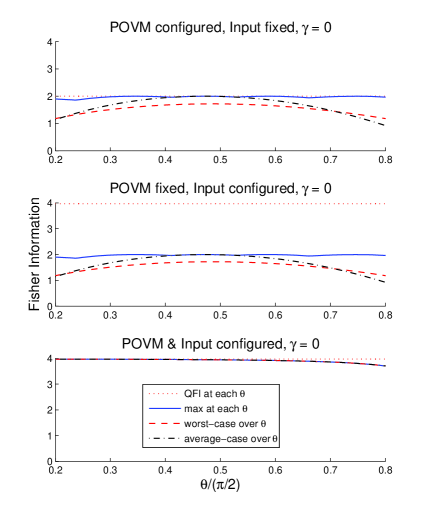
Figure 2: Comparison of configuration constraints with $\gamma=0$

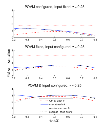
Figure 3: Comparison of configuration constraints with $\gamma=0.25$

Figures 2-3 show the Fisher information as a function of the parameter $\theta$ for the two values of amplitude damping and the three configuration constraints. In each figure the dotted lines are the QFI for each $\theta$ (14). Note that the absolute maximum for the QFI is achieved only for $\gamma=0$ (unitary channel) and using (15) with $H_{0}$ as given above gives $F_{\rm QFI}(\theta)=4$. The solid lines are the maximum achievable for each value of $\theta$ that maximizes the Fisher information under the configuration constraints (13). The dashed lines are what is achieved by using the worst-case distribution of experiments (11), and the dot-dash lines are the average-case distribution of experiments (12).

In all cases, the constrained Fisher information $F(\lambda^{\rm ac},\theta)$, and $F(\lambda^{\rm wc},\theta)$ are relatively close, sometimes nearly coincident to the maximum possible, $F_{\rm max}(\theta)$, and all are lower than the QFI. When both POVM and input are jointly configured the constrained information begins to approach $F_{\rm max}(\theta)$. The curves for the case where only the POVM is configured are generally below those where only the input is configured.

$\gamma$	Configured	Average-Case			Worst-Case
		$\phi/\pi$	$\beta/\pi$	$\lambda^{\rm ac}$	$\phi/\pi$	$\beta/\pi$	$\lambda^{\rm wc}$
0	POVM	.89	0	1	.44	0	.57
	Input	0	.89	1	0	.44	.57
					0	.78	.43
	POVM & Input	.89	.89	1	.89	.89	.89
0.25	POVM	.44	0	1	.78	0	1
	Input	0	.33	1	0	0	.14
					0	.33	.72
					0	1	.14
	POVM & Input	.89	.33	1	.89	.33	.80
					.89	.89	.20

Table 1: Optimal distributions

The numerically non-zero elements of the worst-case and average-case optimal distributions for all the cases are shown in Table 1. By construction, only one input configuration is required for the average-case distribution (10). The worst-case distribution requires up to 3 configurations when $\gamma=0.25$. In this example the configuration angles remain relatively unchanged exhibiting some robustness to the amplitude damping probability $\gamma$. The worst-case distributions change more significantly. Given the relatively close levels of Fisher information for $\theta\in\Theta$, it would seem more prudent to use the single-setting of input and POVM obtained from the average-case optimization. In most experiments there is a penalty in terms of time to reset the configurations.

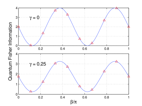
Figure 4: QFI vs. input configuration parameter $\beta$ for $\gamma\in\left\{0,0.25\right\}$. $\triangle$ are the ${N_{\rm input}}=10$ available.

In this example the available input configurations effect the QFI. The solid lines in Figure 4 show the QFI for each value of $\gamma$ vs. the input configuration angle $\beta$ for a large number of samples in the range. The QFI in this case is independent of $\theta$. The triangles show the ${N_{\rm input}}=10$ available values. The solid lines indicate that multiple inputs can achieve the bound whereas the restricted set forces a unique maximum which does not necessarily occur at the true maximum. For example, as seen in the top plot for $\gamma=0$, the constrained maximum is near the global maximum ($F_{\rm QFI}(\theta)=4$). This is achieved only in the case with $\gamma=0$ and clearly over bounds the plot for $\gamma=0.25$. As might be expected, a perturbation of the unitary channel, in this case via amplitude damping, makes it harder to attain the maximum possible QFI. Observe also that if the inputs were further constrained, say $\beta/\pi\in\left\{0,0.2,0.5,0.8\right\}$, then the achieved QFI would not be nearly as close to the maximum possible. The analysis of this examples thus provides the designer with information about the limit of performance of the system. If the potential performance increase over what is available under the constraints on instrumentation is significant, then a more flexible instrumentation might be considered worthwhile.

V Conclusion

We have shown that maximizing the precision in estimating a single parameter in a quantum system subject to input and POVM constraints reduces to a linear program for both what is defined here as a worst-case and average-case objective. For the average-case, the solution to the linear program can be expressed analytically and involves a simple search, i.e., find the largest element of an easily computed vector. Both solutions provide different levels of Fisher information over the range of anticipated parameter variation. Comparing these constrained solutions to the best possible under the constraints as well as to the QFI gives an indication of the performance limitations imposed by the constraints.

Future efforts will consider the effect of entanglement and multi-parameter estimation.

References

- (1) A. S. Holevo, Probabilistic and Statistical Aspects of Quantum Theory (North-Holland, Amsterdam, 1982).
- (2) S. Braunstein and C. Caves, Phys. Rev. Lett. 72, 3439 (1994).
- (3) M. Sarovar and G. J. Milburn, J. Phys. A: Math. Gen. 39, 8487 (2006).
- (4) V. Giovannetti, S. Lloyd, and L. Maccone, Phys. Rev. Lett. 96, 010401 (2006).
- (5) S. Boixo, S. Flammia, C. Caves, and J. Geremia, Phys. Rev. Lett. 98, 090401 (2007).
- (6) A. Shaji and C. M. Caves, Phys. Rev. A 76, 032111 (2007).
- (7) H. Cramér, Mathematical Methods of Statistics (Princeton Press, Princeton, NJ, 1946).
- (8) S. Boyd and L. Vandenberghe, Convex Optimization (Cambridge University Press, Cambridge, UK, 2004).
- (9) R. L. Kosut, I. A. Walmsley, and H. Rabitz, quant-ph/0411093 (2004).
- (10) M.A. Nielsen and I.L. Chuang, Quantum Computation and Quantum Information (Cambridge University Press, Cambridge, UK, 2000).