Numerical evolution of radiative Robinson-Trautman spacetimes

Abstract

The evolution of spheroids of matter emitting gravitational waves and null radiation field is studied in the realm of radiative Robinson-Trautman spacetimes. The null radiation field is expected in realistic gravitational collapse, and can be either an incoherent superposition of waves of electromagnetic, neutrino or massless scalar fields. We have constructed the initial data identified as representing the exterior spacetime of uniform and non-uniform spheroids of matter. By imposing that the radiation field is a decreasing function of the retarded time, the Schwarzschild solution is the asymptotic configuration after an intermediate Vaidya phase. The main consequence of the joint emission of gravitational waves and the null radiation field is the enhancement of the amplitude of the emitted gravitational waves. Another important issue we have touched is the mass extraction of the bounded configuration through the emission of both types of radiation.

I Introduction

An outstanding problem of classical general relativity is the gravitational wave emission from the collapse of bounded distributions of matter to form black holesmtw . The knowledge of the underlying physical processes in which the nonlinearities of the field equations play a determinant role will be very useful in connection to the current efforts toward the detection of gravitational waves. Realistic models of collapse must include rotation as well as the emission of radiationbaiotti due to processes involving the matter fields inside the bounded source, therefore constituting a formidable problem to be tackled numericallybonazzola . In particular it will be of enormous importance to know the amount of mass radiated away by gravitational waves, the generated wave fronts and the influence of other radiative fields, such as electromagnetic and neutrino fields, on the emission of gravitational waves.

Recently, we have studied the full dynamics of Robinson-Trautman (RT) spacetimesrt that can be interpreted as describing the exterior spacetime of a collapsing bounded source emitting gravitational wavesoliv1 . The process stops when the stationary final configuration, the Schwarzschild black hole, is formed, and this happens for all smooth initial data. An interesting possibility in extending this model is to include a null radiation field that can represent an incoherent superposition of electromagnetic waves, neutrino or massless scalar fields. Therefore, our objective here is to evolve the class of Robinson-Trautman geometries filled with pure radiation fieldrt_radiation that correspond to the exterior spacetimes of spheroids of matter which are astrophysically reasonable distributions of matter.

The paper is organized as follows. In Section 2 we present the equations governing the evolution of radiative Robinson-Trautman spacetimes, along with the invariant characterization of gravitational waves through the Peeling theorem. In Section 3 we derive the initial data for Robinson-Trautman that represent the exterior spacetime of uniform and non-uniform spheroids of matter. The procedure of integrating the set of nonlinear equations through the Galerkin method is outlined in Section 4. Although not presenting the details here, we have improved the implementation of the Galerkin method in which the issues of accuracy and convergence were discussed in Ref. oliv3 . Section 5 is devoted to the presentation and discussion of the dynamics of the model and the gravitational wave patterns. The issue of mass loss due to emission of gravitational waves is discussed in Section 6, where we suggest the validity of a non-extensive relation between the fraction of mass extracted and the mass of the formed black hole. Finally, in Section 6 we present a summary of the main results as well as future perspectives. The linear approximation of the field equations is included in the appendix. Throughout the paper we use units such that $8\pi G=c=1$.

II Basic aspects of the radiative Robinson-Trautman spacetimes

The Robinson-Trautman metric can be expressed as

$$ds^{2} = \left(\lambda(u,\theta)-\frac{2m_{0}}{r}+2r\frac{\dot{K}}{K}\right)du^{2}+2dudr$$ (1)

$$-r^{2}K^{2}(u,\theta)(d\theta^{2}+\sin^{2}\theta d\phi^{2}),$$

where $u$ is a null coordinate such that $u={\rm constant}$ denotes null hypersurfaces generated by the rays of the gravitational field, and that foliates the spacetime globally; $r$ is an affine parameter defined along the null geodesics determined by the vector $\partial/\partial r$ and $m_{0}$ is a constant. The angular coordinates $(\theta,\phi)$ span the spacelike surfaces $u=$ constant, $r=$ constant commonly known as the 2-surfaces. In the above expression dot means derivative with respect to $u$ and $\lambda(u,\theta)$ is the Gaussian curvature of the 2-surfaces. Note that we are assuming axially symmetric spacetimes admitting the Killing vector $\partial/\partial\phi$.

The Einstein equations for the Robinson-Trautman spacetimes filled with a pure radiation field are reduced to

$$\lambda(u,\theta)=\frac{1}{K^{2}}-\frac{K_{\theta\theta}}{K^{3}}+\frac{K_{\theta}^{2}}{K^{4}}-\frac{K_{\theta}}{K^{3}}\cot\theta$$ (2)

$$-6m_{0}\frac{\dot{K}}{K}+\frac{(\lambda_{\theta}\sin\theta)_{\theta}}{2K^{2}\sin\theta}=E^{2}(u,\theta),$$ (3)

where the subscript $\theta$ denotes derivative with respect to the angle $\theta$. The function $E^{2}(u,\theta)$ appears in the energy-momentum tensor of the pure radiation field as

$$T_{\mu\nu}=\frac{E^{2}(u,\theta)}{r^{2}}\,l_{\mu}l_{\nu},$$ (4)

where $l_{\mu}=\delta_{\mu}^{0}$ is a null vector aligned along the degenerate principal null direction. The vacuum RT spacetime is recovered if $E(u,\theta)=0$, and the case in which the energy density does not depend on $\theta$ corresponds to the pure homogeneous radiation field.

The structure of the field equations is typical of the characteristic evolution scheme: Eq. (2) is a constraint or a hypersurface equation that defines $\lambda(u,\theta)$, and Eq. (3) or the RT equation governs the dynamics of the gravitational field. In other words, from the initial data $K(u_{0},\theta)$ the constraint equation determines $\lambda(u_{0},\theta)$, and after fixing the function $E^{2}(u,\theta)$, the RT allows to evolve the initial data. Therefore, this equation will be the basis of our analysis of the gravitational wave emission together with a radiation field.

Several important works have been devoted to the evolution of the vacuum RT spacetimes focusing on the issue of the existence of solutions for the full nonlinear equation. The most general analysis on the existence and asymptotic behavior of the vacuum RT equation was given by Chrusciel and Singletonchru . They have proved that for sufficiently smooth initial data the spacetime exists globally for positive retarded times, and converges asymptotically to the Schwarzschild metric. Bicák and Perjésbicakperjes extended the Chrusciel-Singleton analysis considering the pure homogeneous radiation field, and established that for sufficiently smooth initial data the RT spacetime approaches asymptotically to the Vaidya solutionvaidya . In fact the spherically symmetric Vaidya metric is a particular solution of the field equations (2) and (3). Then, by assuming that $K(u,\theta)=K(u)$, it follows from Eq. (2) that $\lambda(u,\theta)=K^{-2}(u)$, and the RT equation yields

$$K(u,\theta)=K(u)\propto\exp\left(-\frac{1}{6m_{0}}\,\int E^{2}(u)du\right).$$

The usual form of the Vaidya metric is recovered after a suitable change of coordinates, $u\rightarrow\bar{u}=\int du/K(u)$, for which the following expression for the mass function emerges

$$M_{Vaidya}(\bar{u})=m_{0}K^{3}(\bar{u}).$$ (5)

By assuming further that the bounded collapsing matter emits radiation for some time until the Schwarzschild final configuration is settled down, its mass will be given by $M_{Schw}=m_{0}K_{f}^{3}$, where $K_{f}$ is the final value of $K(u,\theta)$.

It will be important to exhibit a suitable expression for the total mass-energy content of the RT spacetimes which we identify as the Bondi mass. To accomplish such task it is necessary to perform a coordinate transformation to a coordinate system in which the metric coefficients satisfy the Bondi-Sachs boundary conditions (notice that in the RT coordinate system the presence of the term $2r\dot{K}/K$ does not fulfill the appropriate boundary conditions). We basically generalize the procedure outlined by Foster and Newmanfn to treat the linearized problem, whose details can be found in Ref. oliv2 ; gonnakramer . The result of interest is that Bondi’s mass function can be written for any $u$ as $M(u,\theta)=m_{0}K^{3}(u,\theta)+\rm{corrections}$, where the correction terms are proportional to the first and second Bondi-time derivatives of the news function; furthermore at the initial null surface $u=u_{0}$ these correction terms can be set to zero by properly eliminating an arbitrary function of $\theta$ appearing in the coordinate transformations from RT coordinates to Bondi’s coordinates. Thus, the total Bondi mass of the system at $u=u_{0}$ is given by

$$M(u_{0})=\frac{1}{2}m_{0}\,\int_{0}^{\pi}\,K^{3}(u_{0},\theta)\,\sin\theta d\theta.$$ (6)

As a matter of fact, this expression will be very important to our analysis of the mass extraction by gravitational waves.

The invariant characterization of gravitational waves in RT spacetimes relies on the Peeling theorem, which is based on the algebraic structure of the vacuum curvature tensor of the geometry (1). The Peeling theorempeeling states that the vacuum Riemann or the Weyl tensor of a gravitationally radiative spacetime generated by a bounded source expanded in powers of $1/r$ has the general form

$$R_{ABCD}=\frac{N_{ABCD}}{r}+\frac{III_{ABCD}}{r^{2}}+\frac{D_{ABCD}}{r^{3}}+...$$ (7)

where $r$ is the parameter distance along the null vector field $\partial/\partial r$, and the curvature tensor is evaluated in an appropriate tetrad basisoliv1 . The quantities $D_{ABCD}$, $III_{ABCD}$ and $N_{ABCD}$ are of algebraic type D, type III and type N in the Petrov classificationpetrov and have the vector field ${\partial}/{\partial}r$ as a principal null direction. The above equation contains the information about the radiation zone, that is, for large values of the distance parameter $r$ the vacuum Riemann tensor is dominated by $N_{ABCD}/r$, which is Petrov type $N$. In other words, the field looks like a gravitational wave at large distances, in which the wave fronts are the $u$=const. surfaces with ${\partial}/{\partial}r$ its propagation vector. In this vein, the non-vanishing of the scalars $N_{ABCD}$ is taken as an invariant criterion for the presence of gravitational waves in the wave zone.

For the RT spacetimes filled with a pure radiation field the non-vanishing components of the Weyl tensor are

$$W_{2323}=-W_{0101}=2W_{0212}=-\frac{2m_{0}}{r^{3}},$$

$$W_{0323}=\frac{\lambda_{\theta}}{2Kr^{2}}$$

$$W_{0303}=-\frac{D(u,\theta)}{r}-\frac{A(u,\theta)+E^{2}(u,\theta)}{r^{2}},$$ (8)

$$W_{0202}=-\frac{D(u,\theta)}{r}+\frac{A(u,\theta)-E^{2}(u,\theta)}{r^{2}},$$

where the functions $A(u,\theta)$ and $D(u,\theta)$ are given by

$$A(u,\theta)=\frac{1}{4K^{2}}\left(\lambda_{\theta\theta}-2\frac{\lambda_{\theta}K_{\theta}}{K}-\lambda_{\theta}\cot\theta\right)$$ (9)

$$D(u,\theta)=\frac{1}{2K^{2}}\frac{\partial}{\partial u}\left[\frac{K_{\theta\theta}}{K}-\frac{K_{\theta}}{K}\cot\theta-2\left(\frac{K_{\theta}}{K}\right)^{2}\right].$$ (10)

Therefore the function $D(u,\theta)$ characterizes the wave zone and allows us to determine the evolution of the angular pattern of the emitted waves. It is important to remark that Gönna and Kramergonnakramer have demonstrated, after performing a suitable coordinate transformation to the Bondi variables, that the news function of the RT metric is directly related to $D(u,\theta)$. Notice that both expressions are the same as found in the vacuum case, but the influence of the radiation field on the gravitational wave amplitude is indirect since the evolution of $K(u,\theta)$ is altered by the inclusion of $E(u,\theta)$.

III Initial data: spheroids in RT spacetimes

A very important task is the construction of physically plausible initial data $K(u_{0},\theta)$ for the RT equation. We have chosen the family of prolate or oblate spheroids due to their astrophysical relevance, and also motivated by the works of Lin et allin and Shapiro and Teukolskyshapiro that have analyzed the collapse of gas spheroids in Newtonian and relativistic situations, respectively. Eardleyeardley_spheroids have focused on the collapse of marginally bound spheroids and the efficiency of the gravitational wave emission in this process. In order to construct the initial data correspondent to spheroids, we follow the procedure outlined in Ref. oliv5 . We start with the oblate spheroid initial data whose initial step is to consider the oblate spheroidal coordinates $(\zeta,\theta,\phi)$ defined by

$$x = a\sqrt{\zeta^{2}+1}\sin\theta\cos\phi$$

$$y = a\sqrt{\zeta^{2}+1}\sin\theta\sin\phi$$ (11)

$$z = a\zeta\cos\theta$$

where $a$ is a constant, $(x,y,z)$ are the usual cartesian coordinates and $\zeta\geq 0$, $0\leq\theta\leq\pi$ and $0\leq\phi\leq 2\pi$. Notice that the surfaces $\zeta=$constant represent oblate spheroids described by $\frac{x^{2}+y^{2}}{a^{2}(1+\zeta^{2})}+\frac{z^{2}}{a^{2}\zeta^{2}}=1$.

The flat line element of the spatial surface $\Sigma$ is ${}^{(3)}ds^{2}=dx^{2}+dy^{2}+dz^{2}$ expressed in the above set of coordinates becomes ${}^{(3)}ds^{2}=a^{2}\Big{[}(\zeta^{2}+\cos^{2}\theta)\Big{(}\frac{d\zeta^{2}}{1+\zeta^{2}}+d\theta^{2}\Big{)}+(1+\zeta^{2})\sin^{2}\theta d\phi^{2}\Big{]}.$ Then, as the next step $\Sigma$ is taken as the spacelike surface of initial data with geometry defined by the following line element

$${}^{(3)}ds^{2} = K^{2}(\zeta,\theta)\Big{[}(\zeta^{2}+\cos^{2}\theta)\Big{(}\frac{d\zeta^{2}}{1+\zeta^{2}}+d\theta^{2}\Big{)}+$$ (12)

$$(1+\zeta^{2})\sin^{2}\theta d\phi^{2}\Big{]}.$$

We assume time-symmetric initial data such that the vacuum Hamiltonian constraintyork becomes

$$\nabla^{2}\,\Psi=0,$$ (13)

where $K=\Psi^{2}(\zeta,\theta)$ and $\nabla^{2}$ is the flat space Laplace operator in oblate spheroidal coordinates. The simplest solution of this equation is $\Psi$=constant that implies $K$=constant describing the Schwarzschild configuration. The general solution of this equation can expanded as a series of the product of Legendre polynomials of first and second kindlebedev . By imposing suitable boundary conditions we obtain the following non-flat solution of (13) that represents the exterior region of an oblate with uniform mass distribution

$$\Psi(\zeta,\theta)=\sqrt{a}\Big{[}1+\frac{B_{0}}{2a}\Big{(}\alpha(\zeta)+\frac{1}{2}\beta(\zeta)P_{2}(\cos\theta)\Big{)}\Big{]},$$ (14)

where $\alpha(\zeta)=\arctan(1/\zeta)$, $\beta(\zeta)=(1+3\zeta^{2})\arctan(1/\zeta)-3\zeta$, $P_{2}(\cos\theta)$ is the second-order Legendre polynomial and $B_{0}$ is a constant. The physical meaning of $B_{0}$ becomes clear after rewriting the metric (12) with the above solution for large $\zeta$ (which implies in $r\approx a\zeta$), or

$${}^{(3)}ds^{2}=\Big{(}1+\frac{B_{0}}{2r}+{\cal{O}}(r^{-3})\Big{)}^{4}ds^{2}_{\rm{flat}}.$$ (15)

Therefore $B_{0}$ is identified as the mass of the oblate spheroid as measured by an observer at infinity.

At this point we can extract the initial data for the RT dynamics. Notice that the conformal function (14) evaluated at $\zeta=\zeta_{0}$=constant contains all the information on the initial data correspondent to the exterior region of an oblate spheroid. Then, since the degrees of freedom of the vacuum gravitational field are contained in the conformal structure of 2-spheres embedded in a 3-spacelike surface, as established by D’Inverno and Stacheldinverno that studied the initial formulation of characteristic surfaces, we are led to adopt the following initial data

$$K(\zeta_{0},\theta)=a\Big{[}1+\frac{B_{0}}{2a}\Big{(}\alpha_{0}+\frac{1}{2}\beta_{0}P_{2}(\cos\theta)\Big{)}\Big{]}^{2},$$ (16)

with $\alpha_{0}=\alpha(\zeta_{0})$ and $\beta_{0}=\beta(\zeta_{0})$.

A similar procedure can be done in order to derive the initial data representing the exterior spacetime of a uniform prolate spheroid. Now we start by introducing prolate spheroidal coordinates $(\xi,\theta,\phi)$arfken $x=a\sqrt{\xi^{2}-1}\sin\theta\cos\phi$, $y=a\sqrt{\xi^{2}-1}\sin\theta\sin\phi$, $z=a\xi\cos\theta$, in which $\xi\geq 1$ and the surfaces $\xi=\xi_{0}$=constant define prolate spheroidal spheroids with foci at the points $(0,0,\pm a)$. After a straightforward calculation following the same steps for the case of the oblate spheroids we obtainlebedev

$$K(\xi_{0},\theta)=a\Big{[}1+\frac{B_{0}}{2a}\Big{(}\bar{\alpha}_{0}-\frac{1}{2}\bar{\beta}_{0}P_{2}(\cos\theta)\Big{)}\Big{]}^{2},$$ (17)

where $\bar{\alpha}_{0}=1/2\ln[(\xi_{0}+1)/(\xi_{0}-1)]$ and $\bar{\beta}_{0}=1/2(3\xi_{0}^{2}-1)\ln[(\xi_{0}+1)/(\xi_{0}-1)]-3\xi_{0}$.

It is possible to go further and establish a more general initial data that can be interpreted as describing the exterior spacetime of a spheroid endowed with a non-uniform distribution of matter. It can be shown that if one considers a prolate spheroid, for instance, the initial data can be generically expressed as

$$K(\xi_{0},\theta) = a\Big{[}1+\frac{B_{0}}{2a}\Big{(}\bar{\alpha}_{0}-\frac{1}{2}\bar{\beta}_{0}P_{2}(\cos\theta)\Big{)}+$$ (18)

$$\sum_{n=0}^{\infty}\,a_{n}P_{n}(\cos\theta)\Big{]}^{2},$$

where the closed expression for the additional term depends upon the way the matter inside the spheroid is distributed. When studying the consequences of such an initial data we will choose a suitable exact function of $\theta$ instead the above generic expression.

So far the initial data we have derived describe the vacuum exterior spacetime of bounded matter distributions. The derivation of the initial data for non-vacuum exterior spacetimes is a considerable difficult task due to the fact that we have to solve nonlinear constraint equationsyork instead of the Laplace equation whose analytical solution could be obtained. In this situation we assume that the same initial data as derived previously is extended to describe the exterior spacetime filled with pure radiation field, such that this model can account the collapse of a spheroid mass distribution emitting non-gravitational radiation.

IV Nonlinear approach: implementing the Galerkin method

In order to integrate numerically the field equations (2) and (3) we have applied the Galerkin methodgalerkin . For the sake of completeness we briefly outline here the procedure found in Refs. oliv1 ; oliv3 and improved in Ref. oliv3 . Accordingly, the first step to establish the following Galerkin decomposition

$$K_{a}^{2}(u,x)=A_{0}^{2}\,{\rm e}^{Q(u,x)}=A_{0}^{2}\,{\exp}\left(\sum_{k=0}^{N}\,b_{k}(u)P_{k}(x)\right),$$ (19)

where a new variable $x=\cos\theta$ was introduced; $N$ is the order of the truncation, and $b_{k}(u)$, $k=0,1,...,N$ are the modal coefficients. The Legendre polynomials $P_{k}(x)$ were chosen as the set of basis functions of the projective space, whose internal product is

$$\left<P_{j}(x),P_{k}(x)\right>\equiv\int_{-1}^{1}\,P_{j}(x)P_{k}(x)\,dx=\frac{2\,\delta_{kj}}{2k+1}.$$

The next step is to substitute Eq. (19) into Eq. (2) to obtain an approximate expression for $\lambda(u,x)$,

$$\lambda_{a}(u,x)=\frac{{\rm e}^{-Q(u,x)}}{A_{0}^{2}}\,\left(1+\sum_{k=0}^{N}\,\frac{1}{2}k(k+1)b_{k}(u)P_{k}(x)\right).$$ (20)

Eqs. (19) and (20) are now inserted into the RT equation (3) yielding the residual equation

$${\rm{Res}}(u,x) = 6\,m_{0}\,\sum_{k=0}^{N}\,\dot{b}_{k}(u)P_{k}(x)-\frac{1}{A_{0}^{2}}{\rm e}^{-Q(u,x)}\,\times$$ (21)

$$[(1-x^{2})\,\lambda_{a}^{\prime}]^{\prime}+2E^{2}(u,x),$$

where the prime denotes derivative with respect to $x$. In general the residual equation approaches to zero when $N\rightarrow\infty$ meaning that the decomposition (19) tends to the exact $K(u,x)$. The Galerkin method establishes that the projection of the residual equation onto each basis function $P_{n}(x)$ vanishes, or $\left<{\rm{Res}}(u,x),P_{n}(x)\right>=0$. These relations can be cast in the following way

$$\dot{b}_{n}(u) = \frac{(2n+1)}{12m_{0}A_{0}^{2}}\,\left<{\rm e}^{-Q(u,x)}\,[(1-x^{2})\,\lambda^{\prime}]^{\prime},P_{n}(x)\right>$$ (22)

$$-\frac{(2n+1)}{6m_{0}}\left<E^{2}(u,x),P_{n}(x)\right>,$$

where $n=0,1,2..,N$. Therefore, the dynamics of RT spacetimes is reduced to a system of ($N+1$) ordinary differential equations for the modal coefficients, or simply a dynamical system. It is worth of mentioning that the issues of accuracy and efficiency of the dynamical system approach are discussed in Ref. oliv3 .

To integrate the dynamical system (22) we need to provide the initial conditions $b_{k}(u_{0})$, $k=0,1,2,..,N$ that represent the initial data $K(u_{0},x)$ constructed in the last Section (Eqs. (16), (17) and (18)). These initial values are obtained from the Galerkin decomposition of $K(u_{0},x)$ (cf. Eq. (19)), which yields

$$b_{j}(u_{0})=\frac{2\left<\ln K(u_{0},x),P_{j}\right>}{\left<P_{j},P_{j}\right>}.$$ (23)

As we have mentioned in the last Section the simplest form for the initial data correspond to the Schwarzschild solution $K(u_{0},x)={\rm{constant}}$ that is described exactly using the above decomposition in which the only non-vanishing modal coefficient is $b_{0}$. In order to illustrate the effect of increasing the truncation order $N$ we have exhibited the plots of the relative error, $R.E.$, between the approximate and exact expressions for the prolate spheroid described by Eq. (17), that is

$$R.E.=\left|\frac{K(u_{0},x)-K_{a}(u_{0},x)}{K(u_{0},x)}\right|.$$

Note that even for a small truncation order $N=4$ the error is acceptable. In the numerical experiments of the next Section we have fixed $N=14$.

Figure 1: Plot of the relative error between the approximate and exact initial data corresponding to a prolate spheroid for $a=1,\xi_{0}=1.01$ and $B_{0}=2$. The curves correspond to truncations orders $N=4,8,14,20$. Notice that even for the modest truncation $N=4$ the error is acceptable.

V Numerical results

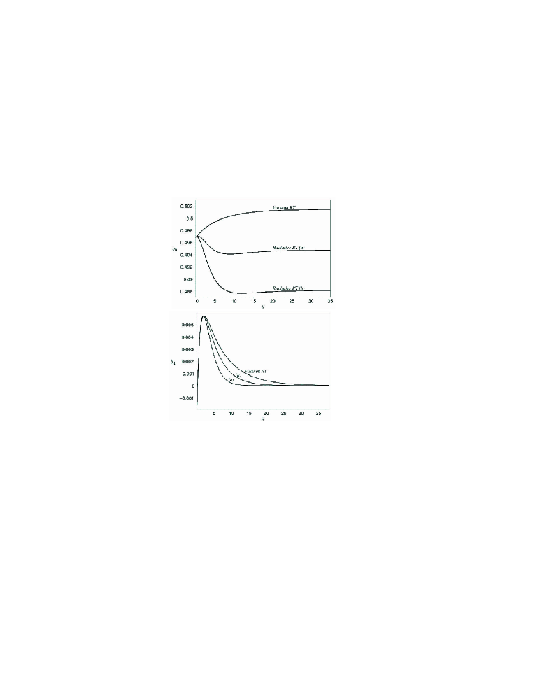
Figure 2: Evolution the modal coefficients $b_{0}(u)$ and $b_{4}(u)$ for the prolate spheroid with $a=1$, $B_{0}=0.1$ and $\xi_{0}=1.01$ for the vacuum and non-vacuum cases. We have considered the homogeneous radiative field $E^{2}(u)=E_{0}^{2}u{\rm{e}}^{-0.5u}$, where for the first and second figures (a) $E_{0}^{2}=0.05,2.0$ and (b) $E_{0}^{2}=0.1,5.0$, respectively.

As we have shown to integrate the set of equation (22) it is necessary to specify the initial conditions determined by the initial data $K(u_{0},x)$ (cf. Eq. 23), and the function $E(u,x)$. We start with uniform spheroid initial data emitting homogeneous radiation (non-gravitational). It is reasonable to impose that $E(u)$ is an arbitrary decreasing function of the retarded time $u$. Amongst several possible choiceshisckock for $E(u)$ we may select $E^{2}(u)=E_{0}^{2}u^{\alpha}\exp(-\beta u)$, where $E_{0}$, $\alpha$ and $\beta$ are positive constants; in particular if $\alpha\neq 0$ we describe a pulsed radiation. For any function $E(u)$ it is important to remark that the influence of the radiation field is basically due to the term $\left<2E^{2}(u),P_{n}(x)\right>=4E^{2}(u)\delta_{n0}$ (see Eq. (22)) that only appears explicitly in the equation for $b_{0}(u)$; the influence on other modal coefficients is indirect through the nonlinear couplings between $b_{0}(u)$ and the remaining ones.

Let us consider the initial conditions $b_{k}(0)$, $k=0,1,..,N$ that correspond to the prolate spheroid described by Eq. (17). By inspecting this expression only even Legendre polynomials are present, and therefore only the even modal coefficients are initially distinct form zero. According to our previous work on the dynamics of vacuum RT spacetimesoliv1 , we have shown that the odd modal coefficients remain unaltered while the even modal coefficients tend to zero asymptotically. The exception is $b_{0}(u)$ that approaches to a constant value, consequently characterizing the Schwarzschild solution as the end state, which in agreement with the analytical works of Chrushiel and Singletonchru . The Schwarzschild mass of the final configuration is given by

$$M_{BH}=m_{0}A_{0}^{3}{\rm{e}}^{\frac{3}{2}b_{0}(u_{f})},$$ (24)

where $b_{0}(u_{f})$ is the asymptotic value of the zeroth modal coefficient, and $u_{f}$ is large but finite. The final mass $M_{BH}$ is always smaller than the initial mass $M(u_{0})$ as should be expected since part of the initial mass is carried away by gravitational waves. We will return to this issue in Section 6.

We have performed several numerical experiments using the set of equation (22) with truncation order $N=14$, and homogeneous radiation field $E^{2}(u)$ with distinct values of $E_{0}$, $\alpha$ and $\beta$. Physically, we have introduced a non-gravitational way of extracting mass that was discussed for the first time by Stachelstachel , but it can be also seem from the linearized formula of mass loss (A). In this way we expect that the mass of the final configuration be smaller than the similar one formed in the absence of the homogeneous radiation field. As a matter of fact, the numerical results have confirmed this feature; the Schwarzschild solution is the asymptotic configuration, that is $b_{2k}\rightarrow 0$, $k\geq 1$, $b_{0}\rightarrow b_{0}(u_{f})={\rm{constant}}$ and smaller than found in the vacuum case. Another important consequence of the homogeneous radiation field is that the approach to the Schwarzschild solution occurs faster than in the vacuum case. In Fig. 2 we have illustrated these features with the plots of the modal coefficients $b_{0}(u)$ and $b_{4}(u)$.

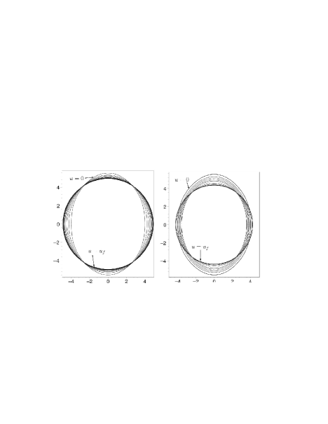
Figure 3: Dynamics of all modal coefficients through the two-dimensional plots of $K(u,x)$ starting from the prolate spheroid initial data ($a=1,B_{0}=0.5,\xi_{0}=1.05$) at $u_{0}=0$, and for several times until the Schwarzschild final configuration (represented by a circle) is formed. The first graph refers to the vacuum RT spacetimes, while the second includes the homogeneous radiation field $E^{2}(u)=4.0\exp(-0.5u)$. One of the effects of the homogeneous radiation field is to produce a Schwarzschild configuration with smaller mass (smaller circle).

The dynamics of all modes together is shown in Fig. 3 for the vacuum and non-vacuum cases. Both graphs consist in sequences of polar plots of $K_{a}(u,x)=A_{0}\exp\left(1/2\sum_{k=0}^{N}\,b_{k}(u)\,P_{k}(x)\right)$ for times $u$ until the Schwarzschild configuration (represented by a circle) is settled down. As expected, the presence of radiation produces a smaller circle due to the additional mass extracted.

The emission of gravitational waves constitutes the central physical aspect of the radiative Robinson-Trautman spacetimes. As we have seen the invariant characterization of the presence of gravitational waves was established on the basis of the Peeling theorem, where $D(u,\theta)$ given by Eq. (10) contains all information about the angular and time dependence of the gravitational wave amplitude in the wave zone. This function can be conveniently expressed in terms of $x=\cos\theta$ and $Q(u,x)$ by

$$D(u,x)=\frac{1}{4A_{0}^{2}}{\rm e}^{-Q(u,x)}(1-x^{2})\,\frac{\partial}{\partial u}\left(Q^{\prime\prime}-\frac{1}{2}Q^{\prime 2}\right)$$ (25)

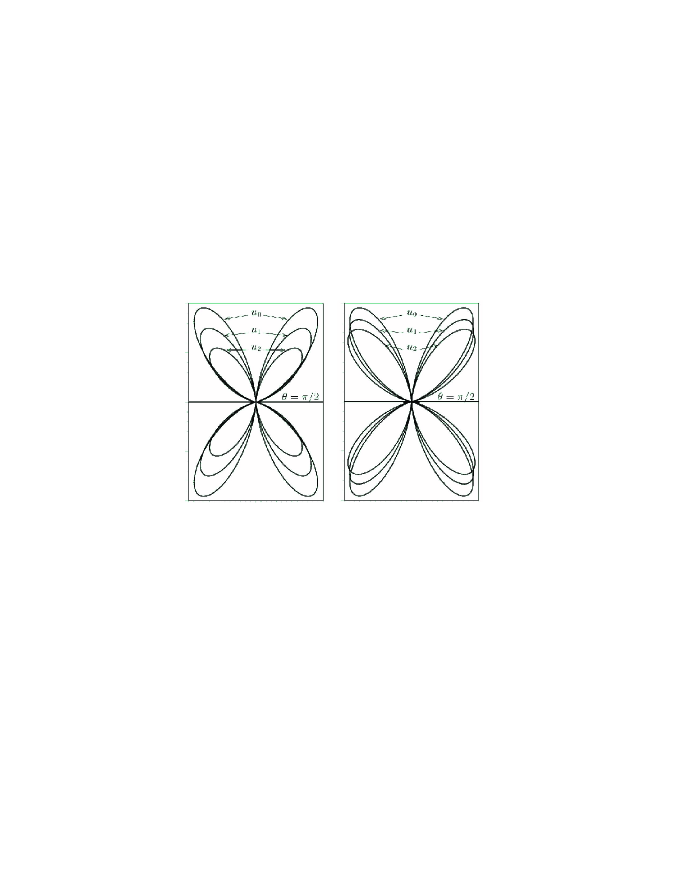
Figure 4: Polar plots showing the evolution of the angular pattern of gravitational waves emitted at the radiation zone for the vacuum (left panel) and non-vacuum cases (right panel), where the quadrupole mode is dominant. The arrows indicate the first instants denoted by $u_{0}=0,u_{1}=0.06,u_{2}=0.18$ in which the angular pattern of $D(u,x)$ were evaluated. The homogeneous radiation field described by $E^{2}(u)=E_{0}^{2}\exp(-0.5u)$ with $E_{0}^{2}=20$ does not affect the pattern of gravitational waves but increases the peaks as indicated above. In both cases the initial conditions correspond to a prolate spheroid with $a=1,\xi_{0}=1.01,B_{0}=0.1$.

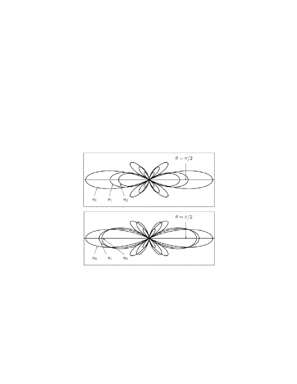
Figure 5: Polar plots showing the evolution of the angular pattern of gravitational waves emitted by an oblate spheroid (16) for vacuum (upper panel) and non-vacuum cases (lower panel). The structure now resembles of that octupole pattern, and as in the case of the prolate spheroid the homogeneous radiation field increases the peaks of gravitation waves. Again the arrows indicates distinct instants $u_{0}=0,u_{1}=0.3,u_{2}=0.6$.

The angular distribution $D(u,x)$ at each instant $u$ is determined from the Galerkin decomposition $Q(u,x)=\sum_{k=1}^{N}\,b_{k}(u)P_{k}(x)$ along with the dynamical system for the modal coefficients. Although not appearing explicitly in the above expression, the radiation field alters the behavior of the modal coefficients and consequently the function $D(u,x)$.

A very useful way of depicting pattern of the gravitational waves at the radiation zone is through by polar plots of $D(u,x)$. In Fig. 4 we present such polar plots evaluated at the initial stages of evolution (as indicated by the arrows) and corresponding to the prolate spheroid initial data (17) for the cases of vacuum and homogeneous radiation field $E^{2}(u)=E_{0}^{2}\exp(-0.5u)$. The patterns of emitted waves have symmetry of reflection by the plane $\theta=\pi/2$ ($x=0$), which is a direct consequence of the absence of all odd modes $b_{2k+1}$. Indeed, the symmetry of the pattern is consistent with the final configuration being a Schwarzschild solution at rest with respect to a distant observer, since no net momentum is carried out by the gravitational waves. In Fig. 5 similar plots are depicted taken into account oblate spheroids initial data.

Two interesting aspects are worth of remarking. The first is the predominant quadrupole structure of the pattern of gravitational waves, and the second is the influence of the homogeneous radiation field that does not alter the pattern of gravitational waves but enhance the amplitude of the peaks. To explain this result we might remember that the radiation field induces a faster decay of the modal coefficients (cf. Fig. 2), and consequently produces higher values of $\dot{b}_{k}$. From Eq. (25), $D(u,x)$ depends directly on the derivatives of the modal coefficients, and therefore its value will be eventually increased. In order to show quantitatively the amplification of the gravitational wave amplitude due to the radiation field, we have evaluated the total flux of gravitational radiation in the wave zone at each instant, which is proportional to

$$\sigma(u)=\int_{-1}^{1}\,|D(u,x)|dx,$$ (26)

according to a distant observer. In Fig. 6 $\sigma(u)$ is plotted for the vacuum and non-vacuum RT spacetimes indicated by the labels (a), (b) and (c) for increasing values of $E_{0}$ taking into account that $E^{2}(u)=E^{2}_{0}u\exp(-0.5u)$.

Figure 6: Influence of the radiation field $E^{2}(u)=E_{0}^{2}u\exp(-0.5u)$ on the behavior of the flux of emitted gravitational waves. We have selected $E_{0}^{2}=3.0,4.0,5.0$ in (a), (b) and (c), respectively. The initial data is the prolate spheroid (17) with $a=1,\xi_{0}=1.01,B_{0}=1.0$.

(a)

(b)

(c)

Figure 7: (a) Behavior of $b_{1}(u)$ indicating that its asymptotic value is distinct from zero. The initial data are non-uniform oblate spheroids characterized by $\zeta_{0}=1,B_{0}=1$ and $\sum_{n=0}^{\infty}\,a_{n}P_{n}(x)=A_{0}\exp(-(x-0.3)^{2})$, where $(i)A_{0}=0.7,(ii)A_{0}=0.2,(iii)A_{0}=0.05$. (b) Plots of the final configuration $K_{a}(x)\equiv\exp(1/2\sum\,b_{k}(u_{f})P_{k}(x))$. These curves are quite well fitted by the analytical expression (27) after choosing appropriate values for $K_{0}$ and $\mu$. In (c) we present the rms error between $K_{a}$ and $K(x)$ for each value of $A_{0}$.

We now turn our attention to a more general initial data that represent the exterior spacetime of a non-uniform prolate spheroid given by Eq. (18). Before discussing the numerical results, it is intuitive to expect that the collapse will proceed in a non-uniform way, meaning that distinct parts of the spheroid will collapse faster/slower than others. As a consequence, the pattern of gravitational waves should not display the same symmetry of reflection by the plane $\theta=\pi/2$ ($x=0$) produced in the case of an uniform spheroid (cf. Figs. 4 and 5). In this case there will be a net flux of momentum carried out by gravitational waves that would be responsible for the recoil of the spheroid.

In order to study more quantitatively this feature, we consider, for the sake of convenience, that the last expression present on the rhs of Eq. (18) is written as $\sum_{n=0}^{\infty}\,a_{n}P_{n}(x)=A_{0}\exp(-(x-x_{0})^{2})$, and that reflects somehow the description of the non-uniformity of the distribution of matter inside the spheroid, or alternatively, a perturbation of the uniform distribution. As a consequence, the Galerkin decomposition yields that all modal coefficients $b_{k}(0)$ are initially distinct from zero. We have first evolved the dynamical system (22) for the vacuum RT spacetimes ($E(u,x)=0$), and contrary to what we have found previously, all modal coefficients tend to constant values asymptotically (for large $u$) as illustrated in Fig. 7(a) with the plot of the modal coefficient $b_{1}(u)$. In Fig. 7(b) we have depicted some of the numerically resulting configurations $K_{a}(x)=\exp\left(1/2\sum_{k=0}^{N}\,b_{k}(u_{f})\,P_{k}(x)\right)$. In order to identify these stationary configurations we recall that the other possible static solution of the RT equation is

$$K(x)=\frac{K_{0}}{\cosh\mu+x\sinh\mu},$$ (27)

where $K_{0}$ and $\mu$ are constants. This solution was found by Bondi et albondi and represents a boosted black hole traveling with velocity $v=\tanh\mu$ along the symmetry axes. The total mass of this configuration is

$$M_{0}=m_{\rm{rest}}\cosh\mu=\frac{m_{\rm{rest}}}{\sqrt{1-v^{2}}},$$ (28)

where $m_{\rm{rest}}=m_{0}K_{0}^{3}$ is the rest mass ($\mu=0$) with respect to a distant observer. Fig. 7(c) shows the rms error between each numerical solution of Fig. 7(b) and the exact solution (27) after convenient choices of $K_{0}$ and $\mu$. Therefore, if all modes are initially excited the asymptotic solution is a boosted black hole.

It is interesting to notice that in the present situation the bounded source is accelerated from the rest at $u=0$ until the emission of gravitational waves finishes. According to Fig. 8, the pattern of gravitational waves exhibits two prominent lobes whose symmetry line is the direction of recoil; also the inclination of the lobes increases with time (cf. Fig. 8)) together with the decrease of their amplitudes. These features are typical of the pattern of waves emitted by an accelerated point particle and are known to form a pattern of bremsstrahlung radiationbremss .

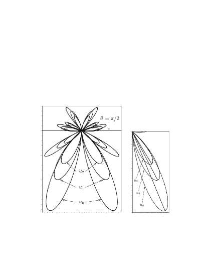
Figure 8: The graph on the left shows the polar plot of $D(u,x)$ exhibiting a typical bremsstrahlung pattern of the gravitational radiation, whereas the detail of one of the lobes evaluated at $u=0$, $u=0.06$ and $u=0.18$ is depicted on the right. Note that two effects are present: the amplitude of the gravitational waves decreases, and the inclination of the lobe changes forming a slightly less sharp forward cone in the direction of motion, as expected from the usual bremsstrahlung radiation.

The final task is to consider inhomogeneous radiation fields which seems to be more consistent in the realm of non-uniform spheroids. Although an inhomogeneous radiation field might arise as a consequence of general internal processes inside the spheroid where the non-uniform matter distribution may play a relevant role, we have not found any physically realistic function to describe such form of radiation. Nonetheless, we can make some considerations about this situation. The dynamics of the modal coefficients will be directly affected by an inhomogeneous radiation field, as it can be seen from the projection $\left<E^{2}(u,x),P_{n}(x)\right>$ that in general does not vanish for any $n$. Possibly, the decay of the modal coefficients to their final values will done faster than in the absence of radiation, as in the case of homogeneous radiation. Besides the additional mechanism of extracting mass of the spheroid provided by the radiation field, there will be also a additional contribution to the total balance of linear momentum. Therefore, the final configuration will be in general a boosted black hole with the following characteristics: its mass is smaller and its velocity can be greater or smaller, respectively, than the mass and velocity of the corresponding boosted black hole found without radiation. Concerning the pattern of gravitational waves, we expect that contrary to the homogeneous case, the inhomogeneous radiation field will change the produced pattern of waves.

VI The mass loss

We have already studied the issue of mass loss due to the emission of gravitational waves beforeoliv1 ; oliv2 ; oliv5 in the realm of vacuum Robinson-Trautman spacetimes. The problem consisted in determining numerically the relation between the fraction of mass lost $\Delta$, or the efficiency of the process, with the final mass of the configuration $M_{BH}$. Here $\Delta$ is defined byeardley_gw

$$\Delta\equiv\frac{|M(u_{0})-M_{BH}|}{M(u_{0})},$$ (29)

where $M(u_{0})$ is the initial mass evaluated according to Eq. (6). As the main result we have shown that the set of numerically generated points $(M_{BH},\Delta)$ can described by the following expression inspired from the Tsallis statisticstsallis ,

$$\Delta=\Delta_{\rm{max}}(1-y^{-\gamma})^{\frac{1}{1-q}},$$ (30)

where $y=M_{BH}/m_{0}A_{0}^{3}$, $\Delta_{\rm{max}}$ is the maximum efficiency, $\gamma$ and $q$ are the other parameters of the distribution law. We have found that for distinct initial data the best fit required that $q\approx 0.5$, the values of $\gamma$ and $\Delta_{\rm{max}}$ depend on the particular choice of the initial data. Here the idea is to revise these results using our improved numerical methodoliv3 , to present some analytical work concerning the relation between $M_{BH}$ and $\Delta$, and to study the consequences of introducing a radiation field.

Before presenting the analytical and numerical results it is important to stress that Eq. (30) may not be considered an artificial relation connecting $\Delta$ and $M_{BH}$. To support this point of view we recall that a black hole can be understood as thermodynamical system in equilibrium, therefore it is a state of maximum entropy. The question we address is the following: given an initial data $K(u_{0},x)$ now viewed as a ”non-equilibrium thermodynamical state”, how much mass must be extracted through gravitational waves such that ”thermodynamical equilibrium” or the black hole formation is achieved? The empirical answer to this question is given by Eq. (30). Nevertheless, the choice of this function is inspired in two aspects: non-extensive relations involving thermodynamical quantities are typical of systems in which a long-range interaction such as gravitation is the relevant onetsallis2 , and the black hole entropy is a non-extensive quantitymaddox .

(a)

(b)

Figure 9: (a) Log-linear plots of the best fit between the points obtained numerically and the non-extensive function (30). The initial data correspond to uniform oblate spheroids with $a=1$, $\zeta=1.0$ (circle), $\zeta=0.5$ (diamond), $\zeta=0.01$ (box), and $B_{0}$ is the free parameter. The best fit required $q\simeq 0.5003$, $q\simeq 0.5007$ and $q\simeq 0.5024$, respectively. (b) Plots of the fraction of mass loss considering uniform prolate spheroids as the initial data whose exterior is vacuum RT and homogeneous radiation field $E^{2}(u)=E_{0}^{2}\exp(-0.5u)$ for (a) $E^{2}_{0}=0.001$, (b) $E^{2}_{0}=0.01$ and (c) $E^{2}_{0}=0.05$. In both cases $y=M_{BH}/m_{0}A_{0}^{3}$.

Let us consider the regime of small mass extraction or equivalently $\Delta\ll\Delta_{\rm{max}}$. As a matter of fact this regime can be approximately described by the linearized equations (cf. Appendix A). Therefore, by setting $E^{2}(u,x)=0$ into the equation that governs the loss of mass (Eq. (A)), $\Delta$ can be calculated analytically:

$$\Delta\simeq\frac{3}{2}(\epsilon_{0}(0)-\epsilon_{0}(u_{f}))+\frac{3}{8}\sum_{k}\,\frac{\epsilon_{k}^{2}(0)}{2k+1}$$ (31)

where $\epsilon(u_{f})$ is the final value of $\epsilon_{0}(u)$. Notice that $\Delta\sim{\cal{O}}(\epsilon^{2})$ implying that $\delta\epsilon_{0}=\epsilon_{0}(u_{f})-\epsilon_{0}(0)\sim{\cal{O}}(\epsilon^{2})$ (indeed, the linear approximation dictates that $\delta\epsilon_{0}=0$). On the other hand, $y=M_{BH}/m_{0}A_{0}^{3}\approx 1+3/2\epsilon_{0}(u_{f})\sim 1+{\cal{O}}(\epsilon)$. Combining these results it follows that

$$y-1\propto\Delta^{1/2}\Rightarrow y\approx 1+{\rm{const.}\Delta^{1/2}}.$$ (32)

By noticing that the nonextensive relation (30) renders $y\approx 1+(\Delta/\Delta_{\rm{max}})^{1-q}/\gamma$ in the limit $\Delta\ll\Delta_{\rm{max}}$, we conclude that $q=0.5$, which is reproduced by the numerical result. Therefore, no matter is the initial data the parameter the regime of very small efficiency dictates that $q=0.5$.

In Fig. 9(a) we have depicted the plots of the points $(M_{BH},\Delta)$ generated numerically with the corresponding best fits of the function (30) (continuous lines). The oblate spheroid (16) was taken as the initial data where $B_{0}$ is the free parameter while $a=1$ and $\zeta=0.01,0.5$ and $1.0$. Note that $\zeta$ is associated to the oblateness through $f=1-\zeta/\sqrt{1+\zeta^{2}}$, a measure of how much the initial distribution of matter deviates from the sphere. Therefore, according to Fig. 9(a) the maximum efficiency attained increases with the oblateness (or decreases with $\zeta$) as should be expected. The numerical values obtained for the maximum efficiency are $\Delta_{\rm{max}}\simeq 0.01038,0.0510,0.2417$, respectively for $\zeta=1.0,0.5,0.01$. It is worth noting that the last maximum efficiency is quite high due to the abnormally enlarged degree of oblateness. For sake of comparation, in the realm of our Solar System the highest oblateness belong to Saturn with $f_{\rm Saturn}\simeq 0.097$ ($\zeta\simeq 2.08$), and Jupiter $f_{\rm Jupiter}\simeq 0.065$ ($\zeta\simeq 2.64$), which are quite small.

We have noticed that one of the most important consequences of the radiation field is to enhance the emission of gravitational waves, increasing, as a consequence the mass loss. The numerical relation between $M_{BH}$ and $\Delta$ is shown in Fig. 9(b), where we have considered for the homogeneous radiation field $E^{2}(u)=E_{0}^{2}\exp(-0.5u)$. The effect of increasing $E_{0}$ is indicated by the successive deviations of the points corresponding to the vacuum case. Although we could not find a function to fit the data, it is possible to estimate analytically the fraction of mass extracted in the late stages dominated by the radiation field, which is described by the Vaidya solution. For the sake of simplicity we consider that asymptotically $\epsilon_{k}\rightarrow 0$, $k\geq 1$ and $\epsilon_{0}\rightarrow$ constant. The late time behavior of $\epsilon_{0}(u)$ can be described approximately by the linear approach such that $\dot{\epsilon}_{0}\approx-1/3m_{0}E^{2}(u)$, which yields, $\delta\epsilon_{0}\approx-E_{0}^{2}/3m_{0}\beta$. It can be shown that the fraction of mass loss is $\Delta\approx 1-\exp(-E_{0}^{2}/2m_{0}\beta)$, which is in agreement with the numerical data as shown in Table 1.

$E^{2}_{0}$	$\Delta_{\rm{teoretical}}$	$\Delta_{\rm{numerical}}$	Relative Error
1	0.0951625820	0.09516258230	$0.315~{}10^{-8}$
0.5	0.0487705755	0.04877057574	$0.492~{}10^{-8}$
0.1	0.0099501663	0.00995016651	$0.213~{}10^{-7}$
0.05	0.0049875208	0.00498752109	$0.577~{}10^{-7}$
0.01	0.0009995002	0.00099950043	$0.230~{}10^{-6}$
0.005	0.0004998750	0.00049987530	$0.600~{}10^{-6}$
0.001	0.0000999950	0.00009999560	$0.599~{}10^{-7}$

VII Final remarks

In this paper we have studied the dynamics of the exterior spacetime of a bounded source emitting gravitational waves and a null radiation field characterized by the function $E(u,\theta)$ (cf. Eq. 4). The joint emission gravitational and some other type of radiation must be expected in a realistic non-spherical collapse. In order to provide a simple model with such features, we have derived the initial data that represent the exterior spacetimes of uniform and non-uniform spheroids of matter in the realm of Robinson-Trautman geometries.

Basically, the main implication of introducing the null radiation field is to produce a faster approach to the final configuration if compared with the case of vacuum ($E(u,\theta)=0$), provided that $E(u,\theta)$ is regular and decays with the retarded time $u$. Indeed, as a consequence of this rapid relaxation towards the stationary configuration, the amplitude of the emitted gravitational waves is enhanced as illustrated in Figs. 4 and 5. In Fig. 6 a more quantitative view of this effect is exhibited. A similar feature can be found, for instance, in the process of formation of supernova in which asymmetric distribution of neutrinos can produce a growth in the gravitational wave emissionneutrino_gw .

The angular distribution of gravitational radiation at the wave zone bestows important information about the initial data and the final configuration. In this vein, distinct initial data will produce distinct pattern of emitted waves, and this fact is clear from Fig. 4 and 5 whose initial data are uniform prolate and oblate spheroids; also the pattern of Fig. 8 is due to non-uniform prolate spheroid. On the other hand, if the pattern has symmetry of reflection by the plane $\theta=\pi/2$ the final configuration will be the Schwarzschild black hole, but if such symmetry is not present as shown in Fig. 8, a boosted black hole will be the end state. As we have seen, the emission of gravitational waves transport a net amount of linear momentum, which is responsible for the recoil of the isolated source due to energy-momentum conservation. In this process the matter source is accelerated producing typical pattern of bremsstrahlungbremss radiation of gravitational waves. The recoil of the remnant (a black hole or a pulsar) resulting from a non-spherical collapse is expected, and has been studied largely in the literature, mainly in the context of supernova explosionssmbh . In particular, according to Eardleyeardley_gw pure gravitational wave recoil in the collapse applies only to the case of collapse to a black hole.

We have also revised the important issue of mass extraction due to the emission of gravitational waves in the realm of vacuum RT spacetimes. Our improved code has confirmed our previous numerical result concerning the non-extensive relation between the fraction of mass extracted and the black hole mass. As a new result we have derived analytically that $q=0.5$, which was confirmed by the numerical experiments.

Finally, the next step of our investigation will be to consider the dynamics of more general axisymmetric spacetimes described in the Bondi problem, where a numerical code based on the Galerkin method is under development. One of our interests is the mass loss due to gravitational wave extraction.

The authors acknowledge the financial support of the Brazilian agencies CNPq and CAPES. We are also grateful to Dr. I. D. Soares for useful comments.

Appendix A Exact solution of the field equations: linear approximation

It is useful to study the linear regime of the field equations of RT spacetimes endowed with radiation field, which is a direct generalization of the Foster and Newmanfn solution for the vacuum case. Basically, we follow the approach of Foster and Newman by assuming that $K(u,\theta)$ is approximated as

$$K^{2}(u,\theta)\simeq A^{2}_{0}\,\left[1+\sum_{n=0}\,\epsilon_{n}(u)\,P_{n}(\cos\,\theta)\right],$$ (33)

where $A_{0}$ is a constant, $|\epsilon_{n}|\ll 1$ and $P_{n}(\cos\,\theta)$ is the Legendre polynomial of order $n$. For the vacuum case Foster and Newman have chosen $n\geq 2$ without loss of generality, since $n=0$ and $n=1$ both represent spheres (considering, of course, the submanifold $r^{2}\,K^{2}\,(d\theta^{2}+\sin^{2}\,\theta\,d\phi^{2})$) that in the latter case has its center displaced at a distance $\epsilon_{1}\,A_{0}$ along the axis of revolution. The linearized field equations are reduced to

$$\sum_{k=0}\,\dot{\epsilon_{n}}\,P_{n}(\cos\,\theta)=-\sum_{n=0}\,k_{n}\epsilon_{n}\,P_{n}(\cos\,\theta)-\frac{E^{2}(u,\theta)}{3m_{0}},$$ (34)

where $k_{n}=\frac{A_{0}^{-4}}{12\,m_{0}}\,(n+2)!/(n-2)!$ is positive for all $n\geq 2$. Let us consider first the homogeneous radiation field, $E^{2}(u,\theta)=E^{2}(u)$, for which the above equation can be rearranged as

$$\dot{\epsilon_{0}}(u)=-\frac{1}{3m_{0}}E^{2}(u),\;\;\dot{\epsilon_{n}}(u)=-k_{n}\epsilon_{n}(u).$$ (35)

The second equation renders immediately $\epsilon_{n}(u)=\epsilon_{n}(0)\,\exp(-k_{n}u)$, $\epsilon_{n}(0)$ being the initial value of $\epsilon_{n}$ evaluated on the hypersurface $u=u_{0}=0$. From this analytical solution all coefficients $\epsilon_{n}\rightarrow 0$ as $u\rightarrow\infty$, which is the same outcome of the vacuum RT geometries. The zeroth mode behaves as $\epsilon_{0}(u)=\epsilon_{0}(0)-\frac{1}{3m_{0}}\,\int_{u_{0}}^{u}\,E^{2}(u)du$, indicating the approach to the Vaidya spacetime asymptotically. In this case, the corresponding line element that characterizes the Vaidya geometry can be obtained after the same coordinate transformation indicated in Section 2.

By considering an inhomogeneous radiation field, we may set $E^{2}(u,\theta)=\sum_{j=0}^{\infty}\,f_{j}(u)P_{j}(\cos\theta)$ to model a physically reasonable form for the energy density of the radiation. Taking into account this expression into Eq. (34), the equations for each mode $\epsilon_{n}(u)$ can be integrated yielding

$$\epsilon_{n}(u)=\epsilon_{n}(0){\rm{e}}^{-k_{n}u}-\frac{1}{3m_{0}}{\rm{e}}^{-k_{n}u}\,\int_{u_{0}}^{u}\,f_{n}(u){\rm{e}}^{k_{n}u}du.$$ (36)

If $n=0$ the solution corresponding to the homogeneous radiation case provided $E^{2}(u)=f_{0}(u)$ is recovered. Again, we also may set $f_{1}(u)=0$ without loss of generality. For those modes $n\geq 2$, the first term on the rhs vanishes in the limit $u\rightarrow\infty$, and the long term behavior of $\epsilon_{n}(u)$ is governed by the second term. It is possible to know the outcome of this asymptotic limit without specifying the functions $f_{n}(u)$, $n\geq 2$. For instance, suppose that all $f_{n}(u)$ are regular in some interval of time say, $u_{0}\leq u\leq u_{1}$, representing a pulsed emission of radiation, or even be decreasing functions such that $\lim_{u\rightarrow\infty}\,f_{n}(u)=0$. As a consequence, the second term on the rhs vanishes asymptotically rendering again $\epsilon\rightarrow 0$ as $u\rightarrow\infty$. Under these conditions and, in addition assuming further that $\lim_{u\rightarrow\infty}\int_{u_{0}}^{u}\,E^{2}(u)du$ is finite, the asymptotic state will be a Schwarzschild black hole.

As a final piece of our study we generalize the original result of Foster and Newman on the change in the total mass-energy of the system. We have followed an alternative approach (instead of using the Newman–Penrose formalism), which consists in expressing the RT equation in terms of the mass function $M(u)\simeq 1/2m_{0}\,\int_{0}^{\pi}\,K^{3}(u,\theta)\sin\theta d\theta$, and taking into account the linearized solution (Eqs. (33) and (34)). After some steps and considering the homogeneous radiation field for the sake of simplicity, we have obtained

$$\frac{\partial M(u)}{\partial u}=-\frac{1}{16A_{0}}\,\sum_{n}\frac{(n+2)!}{(n-2)!}\frac{\epsilon_{n}^{2}(u)}{2n+1}$$

$$-\frac{A_{0}^{3}}{2}E^{2}(u)\left(1+\frac{3}{2}\epsilon_{0}(u)\right).$$ (37)

The first term on the rhs, found by Foster and Newman, means that the mass loss by gravitational wave extraction is a second order effect, while the second term accounts for the mass change due to the radiation field. In this sense, we can interpret the present linearized solution as representing as a bounded source emitting gravitational waves and a null radiation field.

References

- (1) C. W. Misner, K. S. Thorne and J. A. Wheeler, Gravitation (Freeman, San Francisco, 1973).
- (2) L. Baiotti, I. Hawke, P.J. Montero, F. Loeffler, L. Rezzolla, N. Stergioulas, J.A. Font and E. Seidel, Phys. Rev. D71, 024007 (2005).
- (3) S. Bonazzola, E. Gourgoulhon and J. A. Marck, J. Comput. Appl. Math. 109, 433 (1999).
- (4) I. Robinson and A. Trautman, Phys. Rev. Lett. 4, 431 (1960); Proc. Roy. Soc. A265, 463 (1962).
- (5) H. P. de Oliveira and I. Damião Soares, Phys. Rev. D70, 084041 (2004).
- (6) D. Kramer, H. Stephani, E. Herlt and M. A. H. MacCallum, Exact Solutions of Einstein s Field Equations, Cambridge: Cambridge University Press (1980).
- (7) H. P. de Oliveira, E. L. Rodrigues, I. Damião Soares and E. V. Tonini, Int. J. Mod. Phys. C 18, 12, 1853 (2007) (preprint gr-qc/0703007).
- (8) P. Chrusciel, Commun. Math. Phys. 137, 289 (1991); Proc. Roy. Soc. London 436, 299 (1992); P. Chrusciel and D. B. Singleton, Commun. Math. Phys. 147, 137 (1992).
- (9) J. Bicak and Z. Perjes, Class. Quantum Grav. 4, 595 (1987).
- (10) P. C. Vaidya, Proc. Ind. Acad. Sci. A33, 264 (1951).
- (11) J. Foster and E. T. Newman, J. Math. Phys. 8, 189 (1967).
- (12) H. P. de Oliveira and I. Damião Soares, Phys. Rev. D71, 124034 (2005).
- (13) U. von der Gönna and D. Kramer, Class. Quant. Grav. 15, 215 (1998).
- (14) R. Sachs and P. G. Bergmann, Phys. Rev. 112, 674 (1958); R. Sachs, Proc. Roy. Soc. A264, 309 (1961); Proc. Roy. Soc. A270, 103 (1962); E. T. Newman and R. Penrose, J. Math. Phys. 3, 566 (1962).
- (15) H. Bondi, M. G. J. van der Berg and A. W. K. Metzner, Proc. R. Soc. London Ser. A269, 21 (1962).
- (16) A. Z. Petrov, Sci. Nat. Kazan State University 114, 55 (1954).
- (17) C. C. Lin, L. Mestel and F. H. Shu, Astrophys. J. 142, 1431 (1965).
- (18) Stuart L. Shapiro and Saul L. Teukolsky, Phys. Rev. Lett., 66, 994 (1991); Phys. Rev. D45, 2006 (1992).
- (19) D. M. Eardley, Phys. Rev. D 12, 3072 (1975).
- (20) R. F. Aranha, H. P. de Oliveira, I. D. Soares, E. V. Tonini, The Efficiency of Gravitational Bremsstrahlung Production in the Collision of Two Schwarzschild Black Holes, to appear in the International Journal of Modern Physics D (2008).
- (21) J.W. York Jr., The initial value problem and dynamics, in Gravitational Radiation, N. Deruelle and T. Piran, Editors, North-Holland (1983); Gregory Cook, Initial Data for Numerical Relativity, Liv. Rev. in Relativity, 3 (2000); http://www.livingreviews.org/lrr-2000-5.
- (22) N. N. Lebedev, Special Functions and their Applications, Dover Publications, INC. New York (1972).
- (23) R. A. D’Inverno and J. Stachel, J. Math. Phys. 19, 2447 (1978); R. A. D’Inverno and J. Smallwood, Phys. Rev. D22, 1233 (1980).
- (24) G. Arfken, Mathematical Methods for Physicists, , Academic Press (1970).
- (25) P. Holmes, John L. Lumley and Gal Berkooz, Turbulence, Coherent Structures, Dynamical Systems and Symmetry, Cambridge University Press (Cambridge, 1998).
- (26) W. A. Hiscock, Phys. Rev. D23, 2813(1981).
- (27) John Stachel, Phys. Rev. 179, 1251 (1969).
- (28) V. Moncrief, Astrophys. J. 238, 333 (1980).
- (29) Douglas M. Eardley, Theoretical models for sources of gravitational waves, Gravitational Radiation, Nathalie Deruelle and Tsvi Piran, Editors, North-Holland (1983).
- (30) H. P. de Oliveira, I. Damião Soares and E. V. Tonini, Black hole bremsstrahlung in the nonlinear regime of General Relativity, to appear in Proccedings of the Eleventh Marcel Grossman Meeting; Black Hole Bremsstrahlung: can it be an efficient source of gravitational waves?, to appear in the special issue of Int. J. Mod. Phys. D (2006).
- (31) C. Tsallis, J. Stat. Phys. 52, 479 (1988); E. M. F. Curado and C. Tsallis, J. Phys. A24, L69 (1191); 25, 1019 (1992).
- (32) C. Tsallis, Brazilian Journal of Physics, 29, 1 (1999).
- (33) J. Maddox, When entropy does not seem extensive. Nature 365, 103 (1993).
- (34) R. Bingham, R. A. Cairns, J. M. Dawson, R. O. Dendy, C. N. Lashmore-Davies, J. T. Mendonça, P. K. Shukla, L. O. Silva and L. Stenflo, Physica Scripta, T75, 61 (1998); C. Castagnoli, P. Galeotti and O. Saavedra, Astrophys. Space Science 55, 511 (1978); Chris L. Fryer and Kimberly C.B. New, Gravitational waves from gravitational collapse, Living Rev. Relativity 6, (2003), 2; http://www.livingreviews.org/lrr-2003-2.
- (35) Adam Burrow and John Hayes, Phys. Rev. Lett. 76, 352 (1996).