Identifying short motifs by means of extreme value analysis

Abstract

The problem of detecting a binding site – a substring of DNA where transcription factors attach – on a long DNA sequence requires the recognition of a small pattern in a large background. For short binding sites, the matching probability can display large fluctuations from one putative binding site to another. Here we use a self-consistent statistical procedure that accounts correctly for the large deviations of the matching probability to predict the location of short binding sites. We apply it in two distinct situations: (a) the detection of the binding sites for three specific transcription factors on a set of 134 estrogen-regulated genes; (b) the identification, in a set of 138 possible transcription factors, of the ones binding a specific set of nine genes. In both instances, experimental findings are reproduced (when available) and the number of false positives is significantly reduced with respect to the other methods commonly employed.

1 Introduction

Understanding the regulation of gene expression, i.e. the cellular process that controls the amount and timing of appearance of the functional product of a gene, is a challenging task. The expression of a gene is controlled by proteins called transcription factors, which bind to short segments of DNA called binding sites (BSs). BSs are located on long strings of DNA of about 2000 nucleotides (the promoters), upstream of genes. The problem of identifying BSs clearly plays a central role for elucidating the mechanics of gene regulation. The detection of BSs can be carried out experimentally by several high-throughput techniques (see e.g. [1]), though still at very high cost. From such measurements it is possible to infer the frequency with which every nucleotide (A, C, G or T) appears in the BS of a given transcription factor. These data ultimately represent the binding specificity of transcription factors and are usually encoded in the so-called Position-Specific Frequency Matrices (PSFMs) which are catalogued in e.g. the JASPAR [2] and TransFac [3] databases. The entry $f_{ij}$ of a PSFM gives the frequency with which nucleotide $j\in\{\texttt{A},\texttt{C},\texttt{G},\texttt{T}\}$ appears in position $i\in\{1,\ldots,\ell\}$ on the BS ($\ell$ denoting its length) of a given transcription factor, with $\sum_{j}f_{ij}=1$. Thousands of such matrices are available today, covering BSs for many different transcritption factors. Developing effective computational methods to predict the position of BSs on the promoter from the known PSFMs would produce a crucial advantage in terms of identifying new BSs and improving the characterization of binding specificity. From a theorist’s perspective, the question in somewhat simplified terms is the following: given a long string of DNA (the promoter), which short substring is the best putative BS according to the experimental PSFM?

In order to tackle this issue, several methods have been developed and are presently used [4, 5, 6]. Most of them assume a Markovian model as the underlying string generator and consist in (i) a maximum-likelihood procedure to identify candidate substrings on the promoter, and (ii) a statistical test to evaluate the significance of the results against a benchmark in which log-likelihoods are Gaussian-distributed. For short BSs this second step is particularly delicate because their log-likelihoods are expressed as sums of contributions coming from single nucleotides treated independently. Therefore they can not be approximated by Gaussian random variables [7], since the number of terms in the sum is too small. Indeed we show below that the probability distribution function (pdf) of the maximum of the log-likelihoods for short BSs is rarely the extreme value distribution for a Gaussian random variable. The prediction of short BSs thus requires a more precise method that is able to account correctly for large deviations in evaluating their statistical significance.

In this work we apply the standard approach used in statistics to evaluate the distribution of the maximum, i.e. extreme-value theory and particularly the Peak-over-Threshold (POT) method, to estimate the statistical significance of putative BSs. This technique has been employed in financial analysis [8] and meteorology (see e.g. [9]). We firstly test our method by identifying, among 138 transcription factors listed in JASPAR, the ones binding a specific set of skeletal muscle specific genes, reproducing experimental results with a marked reduction of false positives in comparison with other computational methods [10, 11]. Subsequently, we apply it to the detection of a BS that is widely studied experimentally, that is ERE [12] (estrogen responsive element, $\ell=13$), and of two other BSs that are believed to be functionally related to ERE (called AP2 and C/EBP, both $\ell=12$) on a data set of 134 promoters for genes whose expression is altered upon treatment with an estrogen-sensitive growth factor [13].

2 Setup

The basic setting of probabilistic schemes is in general terms as follows. Consider a string of length $L$ drawn from a finite alphabet $\mathcal{A}$. We assume that it can be divided in two parts: a background consisting of $L-\ell$ letters and a motif of length $\ell$ (the BS). These are produced in general by different stochastic models $P_{b}$ and $P_{m}$ (the latter encoded by the PSFM, in the case discussed above). Neglecting all correlations, the probability of observing a certain sequence $S_{k}=\{a_{1},\ldots,a_{L}\}$ of length $L$ including a motif that starts at location $k+1$ is simply

$$P(S_{k}) = \underbrace{\prod_{i=1}^{k}P_{b}(a_{i},i)}_{\text{background}}\underbrace{\prod_{i=k+1}^{k+\ell}P_{m}(a_{i},i)}_{\text{motif}}\underbrace{\prod_{i=k+\ell+1}^{L}P_{b}(a_{i},i)}_{\text{background}}$$ (1)

$$= \prod_{i=1}^{L}P_{b}(a_{i},i)\prod_{i=k+1}^{k+\ell}\frac{P_{m}(a_{i},i)}{P_{b}(a_{i},i)}$$

where $P_{b}(a_{i},i)$ (resp. $P_{m}(a_{i},i)$) represents the probability to observe letter $a_{i}\in\mathcal{A}$ in position $i$ in the background (resp. the motif). It is clear that the motif can be identified as the substring that maximizes the second factor in the right-hand side of (1), or equivalently its logarithm, i.e.

$$W_{k}=\sum_{i=k+1}^{k+\ell}\left[\log P_{m}(a_{i},i)-\log P_{b}(a_{i},i)\right]$$ (2)

since larger values of $W_{k}$ suggest that the string starting at $k+1$ is more likely to be a motif than a common substring. $W_{k}$ is called the score of the substring. Moving $k$ along the string, one can then compute $L-\ell+1$ scores, one for each substring of length $\ell$, and select the one with the highest score as the most likely motif. We shall henceforth denote by $k^{\star}+1$ the starting locus of the score-maximizing substring. Note that multiple maxima may occur.

3 Statistical significance

The problem at this point is to establish how significant $W_{k^{\star}+1}$ is in statistical terms, i.e. how unlikely it is that a particular score has arisen by chance. To this aim, one normally assumes that scores have a Gaussian distribution and are uncorrelated along the sequence (i.e. the $W_{k}$’s are independent random variables for different $k$), and evaluates the likelihood of a given maximum score by employing a Gumbel distribution. Unfortunately, in many cases motifs are short so the number of terms to be summed up in (2) is too small for generating a Gaussian random variable. The distribution of maxima may thus deviate significantly from a Gumbel distribution. To appreciate how the histogram of scores varies with $\ell$ one can study the pdf that emerges by applying artificial PSFMs on random promoters. We have constructed an ensemble of promoters of length $10000$ using the nucleotide frequencies in the human genome as the underlying model. On each of these we tested a different artificial PSFM of size $\ell\times 4$ for $\ell\in\{5,\ldots,32\}$. We have considered two cases: information-rich PSFMs, with non-zero entries only for two (randomly selected) nucleotides for each position; information-poor PSFMs, which have instead entries drawn from a uniform distribution on $[0,1/2]$ (the normalization conditions being obviously enforced). These choices represent limiting cases, since real data are typically in-between these alternatives. For each realization we have carried out a Lilliefors test to probe the normality of the score distribution (other normality tests such as the Jarque-Bera test return a very similar picture). Results for the fraction $\phi$ of samples that do not pass the test are shown in Fig. 1.

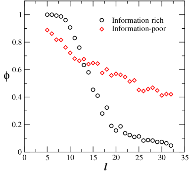
Figure 1: Fraction $\phi$ of random (3^rd order Markovian) realizations that do not pass the Lilliefors Gaussianity test for the score distribution versus motif size $\ell$ (the test is passed by a Gaussian sample). Averages are over $300$ (information-rich PSFM) and $500$ (information-poor PSFM) samples, respectively.

It is clear that the Gaussian hypothesis is inadequate for short motifs in both cases. Remarkably, for information-poor PSFMs it is troublesome also for longer motifs. Note that typical transcription factors BSs have $6\leq\ell\leq 20$. Clearly, it would be important to outperform existing computational methods in the presence of information-poor PSFMs, i.e. when experimental data on motifs are less sharp.

4 Accounting for large deviations

The standard methodology to deal with tail events consists in selecting a high threshold and studying the exceedances of the threshold. The basis for this is a theorem by Pickand [14]. In simplified terms, it states that given a random variable $X$ and a threshold $u>0$, the distribution function of $Y=X-u$ (the ‘excess’ over $u$) is such that

$$\lim_{u\to x_{F}}\text{Pr}\{0<Y\leq u\}:=G_{\xi,\sigma}(y)=1-\left(1+\frac{\xi y}{\sigma}\right)^{-1/\xi}$$ (4)

where $\sigma>0$ is a scale parameter, $\xi$ is the shape parameter of the distribution of the maximum value of the random variable $X$ (see footnote 1), and $x_{F}$ is the right extremum of the distribution function $F(x)=\text{Pr}\{X<x\}$, defined by $x_{F}\equiv\text{inf}\{x:F(x)=1\}$. $G_{\xi,\sigma}$ is called the generalized Pareto distribution (GPD). In other words, the GPD is a good approximation for the distribution of excesses of a random variable over sufficiently high thresholds. Hence, given the set of scores $\{W_{k}\}$ and a threshold $u$, one can obtain estimates $\overline{\xi}$ for $\xi$ and $\overline{\sigma}$ for $\sigma$ by fitting the distribution of excesses over $u$ to a GPD. With $\overline{\xi}$ and $\overline{\sigma}$ it is possible to evaluate the probability to observe a score larger than $u$ using (3). Clearly, the smaller is this quantity, the more significant is the result from a statistical viewpoint. The parameter estimates will however depend on the chosen threshold, i.e. $\overline{\xi}\equiv\overline{\xi}(u)$ and $\overline{\sigma}\equiv\overline{\sigma}(u)$. The problem now consists in choosing $u$ optimally, so that the condition for the validity of Pickand’s theorem is verified with good accuracy and one still has enough data above the threshold to be able to estimate the unknown parameters. As well explained in [8], to this aim one can resort to the following property: let $x_{1},\ldots,x_{n}$ be $n$ independent realizations of a random variable with unknown pdf $F$, and let

$$e_{n}(u)=\frac{\sum_{i=1}^{n}(x_{i}-u)\theta(x_{i}-u)}{\sum_{i=1}^{n}\theta(x_{i}-u)}$$ (5)

be the sample’s mean excess over a fixed threshold $u$, with $\theta(x)$ Heaviside’s step function. Then, if $F$ is a GPD,

$$e_{\infty}(u)=\frac{\sigma+\xi u}{1-\xi}$$ (6)

This implies that when the empirical plot $e_{n}(u)$ versus $u$ follows approximately a straight line with a certain derivative above a value $\overline{u}$ of $u$, then the excesses over $\overline{u}$ follow approximately a GPD with shape parameter related to the observed derivative. This allows for an optimal selection of $\overline{u}$ and, in turn, of $\overline{\xi}$ and $\overline{\sigma}$.

As said above, once we have estimated these parameters we should evaluate the statistical significance of the scores via (4). This can be accomplished via a Peak-over-Threshold (POT) analysis [8, 15]. Consider the excesses of the scores over $\overline{u}$, $Y_{k}=W_{k}-\overline{u}>0$ (scores that do not exceed $\overline{u}$ are hereafter neglected). Given that the number $N$ of excesses above a threshold is a Poissonian variable (see e.g. [16]), one easily understands that

$$\mathcal{P}_{k} \equiv \text{Pr}\left\{\max_{j\in\{0,1,\ldots,L-\ell\}}Y_{j}>Y_{k}\right\}$$ (7)

$$= 1-\text{Pr}\left\{\max_{j\in\{0,1,\ldots,L-\ell\}}Y_{j}\leq Y_{k}\right\}$$

$$= 1-\exp\left[-\lambda\left(1+\overline{\xi}Y_{k}/\overline{\sigma}\right)^{-1/\overline{\xi}}\right]$$

The additional parameter $\lambda$ coming from the Poisson distribution can be estimated from the data simply as $\lambda=N/(L-\ell+1)$, where $N$ is the actual number of scores falling above $\overline{u}$ in our sample. Clearly, $\mathcal{P}_{k}$’s should be as small as possible for $Y_{k}$ to be close to the maximum. A precise condition for real BSs prediction is discussed below.

5 Application to the detection of ERE

We have analyzed a set of 134 promoters whose expression profile is upmodulated by estrogen, a hormone produced in the ovaries. Estrogen diffuses across the cell membrane into the cell, where it interacts with hormones called estrogen receptors. Once activated by estrogen, receptors act primarily as transcription factors to regulate the expression of certain genes by binding to DNA. Estrogen receptors are widely studied in the biomedical literature since estrogen is related to the development and growth of most types of breast cancers. Indeed, breast cancer monitoring commonly includes tests for expression of the estrogen receptor, and reducing the supply of estrogen is part of breast cancer therapy. The interaction of an estrogen receptor with DNA occurs at a BS called estrogen responsive element (ERE, $\ell=13$). The position of ERE is known experimentally on some promoters but it would be important to extend this knowledge to other genes that are sensitive to estrogen. Furthermore, binding at ERE is believed to be cooperatively linked to binding at two other motifs, called AP2 ($\ell=12$) and C/EBP ($\ell=12$). Whether such motifs are present on all promoters for estrogen-upmodulated genes is however not known.

We have screened our data set for the (known) presence of ERE and for the (to be ascertained) presence of AP2 and C/EBP. The PSFMs for the latter genes have been extracted from the TransFac database. For ERE we have used the PSFM derived in [17]. For the sake of clarity, we have subdivided the 134 genes in two groups: the first contains the 14 genes for which experimental knowledge is available (TFF1, STS, CRKL, NROB2, CYP1B1, FEM1A, CYP4F11, FOXA1, RPS6KL, NRIP1, CTSD, GAPD, GREB1, IGFBP4) [13, 18]; for the remaining 120 genes information is available only from computational studies through the NCBI database [19].

It is now important to discuss the conditions for rejection of a putative motif. Statistically significant substrings of DNA (indexed $k$) should satisfy two conditions. On one hand, the value $\mathcal{P}_{k}^{{\rm(t)}}$ of $\mathcal{P}_{k}$ calculated on the true promoter should be smaller than a confidence level $\mathcal{P}_{c}$, since it would be desirable to minimize the probability of finding a score larger than $W_{k}$. $\mathcal{P}_{c}$ must be chosen so as to guarantee that when the above procedure is applied to an ‘engineered’ promoter containing a certain number of motifs, all of these are detected correctly. In the cases we analyzed, $\mathcal{P}_{c}$ turns out to vary in a range between $0.02$ and $0.001$.

Secondly, $\mathcal{P}_{k}^{{\rm(t)}}$ should be larger than the value $\mathcal{P}_{k}^{{\rm(r)}}$ one would obtain when looking for a real motif on a random promoter, e.g. one drawn uniformly from $\{\texttt{A,C,G,T}\}$, with the same threshold $Y_{k}$ used for the real promoter. This condition enforces the expectation that the score of a certain motif computed on a real DNA sequence should be higher than that computed on a random string of DNA, where the motif can only occur by chance. Statistical accuracy can be increased by considering an ensemble of random promoters rather than just one, and computing $\mathcal{P}_{k}^{{\rm(r)}}$ as the average $\mathcal{P}_{k}$ over the ensemble. Indeed, some random strings will produce larger scores than other strings, so it is important to compare the true promoter directly with the random ones, especially so if the true promoter contains the motif.

The condition that relevant substrings of length $\ell$ starting at locus $k+1$ should satisfy is then

$$\mathcal{P}_{k}^{{\rm(r)}}<\mathcal{P}_{k}^{{\rm(t)}}<\mathcal{P}_{c}$$ (8)

For comparison, we have considered another condition, less stringent than (8), namely that both

$$\mathcal{P}_{k}^{{\rm(r)}}<\mathcal{P}_{c}~{}~{}~{}~{}~{}\text{and}~{}~{}~{}~{}~{}\mathcal{P}_{k}^{{\rm(t)}}<\mathcal{P}_{c}$$ (9)

We shall denote the latter as the weak condition and the former as the strong one. These conditions differ from the one which is commonly used. Indeed, normally one only looks for motifs that are unlikely to appear in a random promoter, i.e. the only significancy criterion is $\mathcal{P}_{k}^{{\rm(r)}}<\mathcal{P}_{c}$. We show below that our setting ultimately allows for a reduction in the number of false positives with respect to other methods, while keeping the same predictive efficiency (e.g. the number of true positives) in test cases.

Ultimately, the algorithm we have used to search for ERE, AP2 and C/EBP on each of the 134 promoters can be summarized as follows.

1. Define $P_{m}$ and $P_{b}$, see (1). The former is given by the experimental PSFMs of ERE, AP2 and C/EBP. For $P_{b}$ we have used a 3-step Markovian model (different choices do not impact results significantly)

2. Compute the scores $\{W_{k}^{{\rm(t)}}\}_{k=0}^{L-\ell}$ for the true promoter and $\{W_{k}^{{\rm(r)}}\}_{k=0}^{L-\ell}$ for an ensemble of random promoters generated via a prescribed Markov model (e.g. randomly and unformly from $\{\texttt{A,C,G,T}\}$).

3. Estimate the optimal parameters $(\overline{u}_{\text{t}},\overline{\xi}_{\text{t}},\overline{\sigma}_{\text{t}})$ for the true promoter and $(\overline{u}_{\text{r}},\overline{\xi}_{\text{r}},\overline{\sigma}_{\text{r}})$ for the random promoters.

4. Calculate the probability $\mathcal{P}_{k}^{\text{(t)}}$ for the true promoter, see (7), and $\mathcal{P}_{k}^{\text{(r)}}$ as the average $\mathcal{P}_{k}$ over the random promoters.

5. Select motifs with index $k$ satisfying the significancy conditions, either (8) or (9).

It is worth noting that more than one substring may pass the significancy tests. In this respect, our choice of computing $\mathcal{P}_{k}^{{\rm(t)}}$, that is of considering the likelihood of observing a particular substring on the real promoter alongside $\mathcal{P}_{k}^{{\rm(r)}}$, allows us to draw sharper conclusions on suboptimal putative motifs since the distribution of the largest scores on real and random DNA should differ if a motif is actually present on the real sequence. The fact that more than one motif may occur obviously doesn’t imply cooperation at the biological level. The method can however be modified to account for this aspect, e.g. to identify pairs of correlated motifs [20].

6 Results

We have detected the presence of ERE on all of the 134 promoters, in agreement with experimental knowledge. In Fig. 2 we display the sequence logo [21] relative to whole data set of 134 promoters.

Figure 2: Sequence logo of ERE emerging from the 134 promoters studied. Top: strong significancy condition. Bottom: weak significancy condition.

This should be compared with the sequence GGTCA$\star\star\star$ TGACC ($\star=$any nucleotide) constructed by inserting the most frequent nucleotide in each position and a $\star$ in positions where, experimentally, every nucleotide can be present. Notice that the sequence is palindromic, in the sense that the first five bases link to the last five in reverse order (with the rules A-T, C-G). It is clear from Fig. 2 that our method recovers this property.

On the contrary the presence of AP2 and C/EBP was not found in all of the 134 genes (see below for details from a reduced data set). The resulting sequence logos are shown in Figures 3 and 4.

Figure 3: Sequence logo of AP2 emerging from the 134 promoters studied. Top: strong significancy condition. Bottom: weak significancy condition.

Figure 4: Sequence logo of C/EBP emerging from the 134 promoters studied. Top: strong significancy condition. Bottom: weak significancy condition.

The former should be compared with the sequence CGCCCGCCGGCG built with the experimentally most frequent nucleotides at every position. Note however that the PSFM for AP2 (from TransFac) includes a small number of known BSs (13 at the time of writing this article). For C/EBP, the sequence logo is to be compared to the experimental highest frequency string [G/A]AATTTGGCAAA, where the first position is occupied by guanine or adenine with the same frequency. (In this case a much larger data sample is available to build the PSFM).

In summary, for the genes we considered the method returns sequences that are in a very good agreement with the available experimental knowledge on BSs.

Let us now consider the restricted data set formed by the 14 genes that have been directly accessed in experiments, at least for ERE. In Table 1 we show the outlook of results for the three motifs we considered.

Gene	ERE	AP2	C/EBP
TFF1	Yes	No	Yes
STS	Yes	No	No
CRKL	Yes	Yes	No
NROB2	Yes	No	Yes
CYP1B1	Yes	No	No
FEM1A	Yes	Yes	Yes
CYP4F11	Yes	Yes	No
FOXA1	Yes	No	Yes
RPS6KL	Yes	No	No
NRIP1	Yes	No	Yes
CTSD	Yes	Yes	Yes
GAPD	Yes	No	No
GREB1	Yes	No	No
IGFBP4	Yes	No	Yes

Table 1: Table representing the presence (Yes) or absence (No) of the ERE, AP2 or C/EBP motif on the genes reported in the first column. Results are shown for the strong significancy condition.

With the strong significancy condition, our prediction is that AP2 and C/EBP are not present on all of the 14 genes, at odds with ERE. An experimental validation is not yet available.

Let us now focus on one gene from the data set, namely GAPD (similar results are obtained for the other genes), and consider ERE. In Fig. 5 we display the probability-probability (PP) and quantile-quantile (QQ) plots for GAPD. The former shows the empirical probability distribution of excesses versus a GPD; the latter focuses on the tails, showing the empirical quantiles of the distribution of excesses extracted from the data on GAPD versus the quantiles estimated from a GPD.

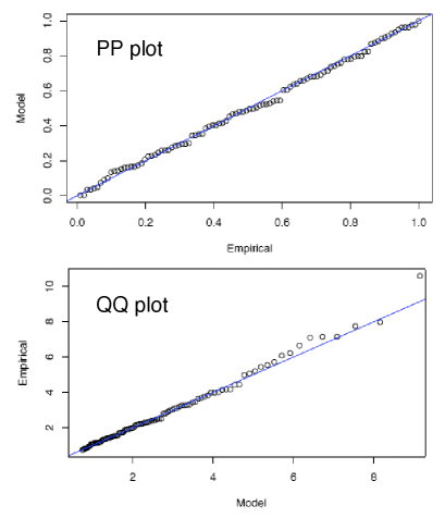
Figure 5: PP-plot (top) and QQ-plot (bottom) for GAPD.

These types of plots provide simple measures of plausibility of a certain model. One sees a convincing agreement between the data and an extreme-value distribution.

7 Application to skeletal-muscle specific genes.

To have an idea of the performance of the method concerning false positives, we have tested it against a known biological benchmark. Specifically, we have considered the full set of nine skeletal-muscle specific genes studied in [11]. This set is well studied experimentally. In particular, it is known that six of the transcription factors from the JASPAR database attach to them [10, 11]. The corresponding motifs have lengths varying from 6 to 12 nucleotides. The best available computational technique, the Tomovic-Oakeley (TO) method [11], takes dependencies between sites into account and is able to identify correctly five of the six factors. Table 2 compares the performance of our algorithm with that of TO and with the best available (to our knowledge) algorithm based on cross-species comparison, ConSite [22].

Gene	ConSite	TO	BT
ALDOA	5/81	5/78	5/70
DES	5/80	5/74	5/70
MYOG	5/87	5/85	6/76
MYL1	6/86	5/75	5/71
TNNI1	5/81	5/78	5/69
MYH7	5/77	4/75	5/76
MYH6	5/83	5/78	5/66
ACTA1	6/80	5/77	5/67
ACTC1	5/84	5/77	5/73

Table 2: Comparison between the performance of the ConSite, the Tomovic-Oakeley (TO, including site dependencies) and the present (BT) algorithm on the set of 9 genes studied in [11]. The first number in each entry gives the number of motifs found on the genes (out of 6), the second gives the number of false positives retrieved in the JASPAR database.

We have chosen our parameters to obtain at least as many true positives as Tomovic-Oakeley. For this setting, the number of false positives is considerably lower in our case.

8 Conclusions

Summarizing, we have accounted for large deviations in the distribution of scores for short BSs by a technique that combines well-known properties of extreme-value distributions and a POT analysis. The importance of fluctuations becomes clear if one studies the score distribution in a random setting. This approach allows for a self-consistent estimation of the statistical significance of putative motifs. The general problem of recognizing a small pattern in a large background however presents many open issues. Among these we mention those that have perhaps a more direct biological implication. First, for obvious reasons it would be important to devise methods yielding a still smaller number of false positives. To this aim a deeper analysis of the performance on artificial data set would be required, so as to improve the estimation of our parameters and to compare the performances of different methods on dependence on $\ell$ and on the structure of the PSFM. Second, one should address the issue of cooperation between transcription factors. In principle, this requires overcoming the independent-nucleotides approximation and developing techniques that account for score correlations along the sequence. Methods accounting for correlations already exist but they need, at present, more parameters and larger data set to obtain a reasonable statistical significance. In our case, it is possible to take into account the effect of dependencies by properly grouping scores and applying extreme-value theory to the block scores. This extension is the object of further work [20]. Clearly, more effective methods would be very welcome and refined statistical and probabilistic tools are likely to play a major role in their development.

- [1] L. Elnitski et al. Genome Res. 16 1455 (2006)
- [2] http://jaspar.genereg.net/
- [3] http://www.gene-regulation.com/pub/databases.html/
- [4] G Pavesi et al., Brief Bionform. 5 217 (2004)
- [5] V. Mustonen and M. Lässig, Proc. Nat’l Acad. Sci. USA 102 15936 (2005)
- [6] GK Sandve and F Drabløs, Biol. Direct 1 11 (2006)
- [7] TL Bailey and M Gribskov, J. Comp. Biology 4 45 (1997)
- [8] P Embrechts, C. Klüppelberg and T Mikosch. Modelling Extremal Events for Insurance and Finance. Springer-Verlag (Berlin, 1997)
- [9] JP Palutikof et al. Meteorological Applications 6 119 (1999)
- [10] M Defrance and H Touzet, BMC Bioinformatics 7 396 (2006)
- [11] A Tomovic and EJ Oakeley, Bioinformatics 23 933 (2007)
- [12] J Wood et al. Mol. Cell. Biology 18 1927 (1998)
- [13] J Laganière et al. Proc. Nat’l Acad. Sci. USA 102 11651 (2005)
- [14] J Pickand. Annals of Statistics 3 119 (1975)
- [15] SG Coles. An introduction to statistical modeling of extreme values. Springer (London, 2001)
- [16] J Hüsler, J. Appl. Prob. 30 877 (1993)
- [17] F Cordero. Thesis, University of Turin (2004) (unpublished)
- [18] V Bourdeau et al. Molecular Endocrinology 18 (2003)
- [19] http://www.ncbi.nlm.nih.gov/
- [20] D Bianchi and B Tirozzi. Forthcoming.
- [21] http://weblogo.berkeley.edu/
- [22] A Sandelin et al Nucl. Acid. Res. 32 W249 (2004)