Simulations of Ultrarelativistic Magnetodynamic Jets from Gamma-ray Burst Engines

Abstract

Long-duration gamma-ray bursts (GRBs) require an engine capable of driving a jet of plasma to ultrarelativistic bulk Lorentz factors of up to several hundred and into narrow opening angles of a few degrees. We use global axisymmetric stationary solutions of magnetically-dominated (force-free) ultrarelativistic jets to test whether the popular magnetic-driving paradigm can generate the required Lorentz factors and opening angles. Our global solutions are obtained via time-dependent relativistic ideal magnetodynamical numerical simulations which follow the jet from the central engine to beyond six orders of magnitude in radius. Our model is primarily motivated by the collapsar model, in which a jet is produced by a spinning black hole or neutron star and then propagates through a massive stellar envelope.

We find that the size of the presupernova progenitor star and the radial profile of pressure inside the star determine the terminal Lorentz factor and opening angle of the jet. At the radius where the jet breaks out of the star, our well-motivated fiducial model generates a Lorentz factor $\gamma\sim 400$ and a half-opening angle $\theta_{j}\sim 2^{\circ}$, consistent with observations of many long-duration GRBs. Other models with slightly different parameters give $\gamma$ in the range $100$ to $5000$ and $\theta_{j}$ from $0.1^{\circ}$ to $10^{\circ}$, thus reproducing the range of properties inferred for GRB jets. A potentially observable feature of some of our solutions is that the maximum Poynting flux in the jet is found at $\theta\sim\theta_{j}$ with the jet power concentrated in a hollow cone, while the maximum in the Lorentz factor occurs at an angle $\theta$ substantially smaller than $\theta_{j}$ also in a hollow cone. We derive approximate analytical formulae for the radial and angular distribution of $\gamma$ and the radial dependence of $\theta_{j}$. These formulae reproduce the simulation results and allow us to predict the outcome of models beyond those simulated. We also briefly discuss applications to active galactic nuclei, X-ray binaries, and short-duration GRBs.

1 Introduction

Models of long-duration gamma-ray bursts (GRBs) require the ejected plasma to move at ultrarelativistic speeds in order to avoid the compactness problem (Piran, 2005). The Lorentz factor required can be as high as $\Gamma\sim 400$ (Lithwick & Sari, 2001), which necessitates a relativistic engine capable of launching plasma with an enormous amount of energy per particle. Achromatic ‘jet breaks’ in the GRB afterglow imply a finite geometric opening angle $\theta_{j}\sim$ a few degrees for a typical long-duration GRB (Frail et al., 2001; Piran, 2005; Zeh et al., 2006). Combined with the observed fluence and the known distance to the source, this gives a typical event energy of $\sim 10^{51}$ ergs, comparable to the kinetic energy released in a supernova explosion.

An ideal engine for producing ultrarelativistic jets with small opening angles, low baryon contamination, and high total energies is a rapidly rotating black hole threaded by a magnetic field and accreting at a hyper-Eddington rate (Narayan et al., 1992; Levinson & Eichler, 1993; Meszaros & Rees, 1997). In such a model, the black hole launches an electromagnetically pure jet via the Blandford-Znajek effect (Blandford & Znajek, 1977). More recently, millisecond magnetars have been seriously considered as another possible source of magnetically-dominated outflows (Usov, 1992; Lyutikov, 2006; Uzdensky & MacFadyen, 2007; Bucciantini et al., 2007). The standard alternative to this magnetic-driving paradigm is neutrino annihilation (Woosley, 1993; MacFadyen & Woosley, 1999), but this mechanism probably does not produce sufficient luminosity to explain most GRBs (Popham et al., 1999; Di Matteo et al., 2002).

Rapidly rotating black holes or millisecond magnetars are thought to be the products of core-collapse (Woosley, 1993; Paczynski, 1998) or binary collisions of compact objects (Narayan et al., 1992, 2001). For failed supernovae, the black hole or magnetar is surrounded by an accretion disc whose corona and wind affect the jet structure through force-balance between the jet and the surrounding gas. In any core-collapse event the jet must penetrate the stellar envelope which can significantly modify the structure of the jet (Woosley, 1993; MacFadyen & Woosley, 1999; Aloy et al., 2000; Narayan et al., 2001; Zhang et al., 2003; Aloy & Obergaulinger, 2007). Indeed, as we demonstrate in this paper, it is likely the case that the properties of the stellar envelope determine the Lorentz factor and opening angle of the jet.

We seek to understand how magnetized rotating compact objects can launch jets that become sufficiently ultrarelativistic and narrow in opening angle to produce long-duration GRBs. To achieve this goal we use the relativistic ideal magnetohydrodynamical (MHD) approximation, which is a valid approximation for much of the GRB jet (e.g., see McKinney 2004). The primary difficulty has been in obtaining a self-consistent global model of the jet that connects the compact object at the center to large distances where the observed radiation is produced. In the context of the collapsar model, this means we need a model that goes all the way from the black hole or neutron star at the center to beyond the outer radius of the Wolf-Rayet progenitor star.

In the past the MHD approximation has been used in numerous analytical efforts aimed at understanding the physics behind acceleration and collimation of relativistic jets. The MHD equations for stationary force balance are highly non-linear, and so analytical studies have been mostly confined to special cases for which the equations can be simplified, e.g. for particular field geometries (Blandford & Znajek, 1977; Beskin et al., 1998; Beskin & Nokhrina, 2006), for asymptotic solutions (Appl & Camenzind, 1993; Begelman & Li, 1994; Lovelace & Romanova, 2003; Fendt & Ouyed, 2004), or for self-similar solutions that allow variable separation (Contopoulos & Lovelace, 1994; Contopoulos, 1995; Vlahakis & Königl, 2003a, b; Narayan et al., 2007). Semi-analytical methods using finite element, iterative relaxation, or shooting techniques have also been used to find jet solutions, such as for spinning neutron stars (Camenzind, 1987; Lovelace et al., 2006) and black holes (Fendt, 1997). Such analytical studies are useful since sometimes one finds families of solutions that provide significant insight into the general properties of solutions (e.g., Narayan et al., 2007).

Time-dependent simulations complement analytical studies by allowing one to investigate a few models with much less restrictive assumptions. In particular, much recent insight into the accretion-jet phenomenon has been achieved within the framework of general relativistic magnetohydrodynamics (GRMHD) via time-dependent numerical simulations (De Villiers et al., 2003; McKinney & Gammie, 2004; McKinney, 2005b; Komissarov, 2005; Aloy & Obergaulinger, 2007). Indeed, numerical simulations of accretion have successfully reproduced collimated relativistic outflows with Lorentz factors reaching 10 (McKinney, 2006b). Within the collapsar model, GRMHD simulations show that magnetized jets can be produced during core-collapse (Mizuno et al., 2004; Liu et al., 2007; Barkov & Komissarov, 2007; Stephens et al., 2008). However, no MHD simulation of core-collapse has yet demonstrated the production of an ultrarelativistic jet. Computationally, such simulations are prohibitively expensive due to the need to resolve vast spatial and temporal scales while at the same time modeling all the physics of the black hole, the accretion disc, the disc wind, and the stellar envelope. A more practical approach, one that we take in this paper, is to replace the real problem with a simplified and idealized model and to explore this model over the large spatial and temporal scales of interest for long-duration GRBs. Such an approach will hopefully demonstrate how ultrarelativistic jets can be produced and will help us assess the applicability of the mechanism to the collapsar model.

In the present work we obtain global solutions of ultrarelativistic magnetically-dominated jets via time-dependent numerical MHD simulations in flat space-time (no gravity). We focus on the relativistic magnetodynamical, or force-free, regime (Goldreich & Julian, 1969; Okamoto, 1974; Blandford, 1976; Lovelace, 1976; Blandford & Znajek, 1977; MacDonald & Thorne, 1982; Fendt et al., 1995; Komissarov, 2001, 2002; McKinney, 2006a), which corresponds to a magnetically-dominated plasma in which particle rest-mass and temperature are unimportant and are ignored. This is a reasonable model for highly magnetized flows (Blandford & Znajek, 1977; McKinney, 2006b). The model parameters we consider are motivated by presupernova stellar models (MacFadyen & Woosley, 1999; Aloy et al., 2000; Zhang et al., 2003; Heger et al., 2005; Zhang et al., 2007) and GRMHD simulations of turbulent accretion discs (McKinney & Gammie, 2004; McKinney & Narayan, 2007a, b). We compare our numerical solutions against self-similar solutions derived by Narayan et al. (2007) and obtain simple physically-motivated formulae for the variation of the Lorentz factor, collimation angle, and Poynting flux along the axis of the jet and across the face of the jet. Based upon our simulations and analytical scalings, we suggest that the terminal Lorentz factor of GRB jets is determined by the size and radial pressure profile of the progenitor star rather than the initial magnetization, for a large range of initial magnetizations.

In §2 we discuss the problem setup and give a brief overview of our numerical method. In §3 we present the numerical results and interpret them in terms of analytical scalings. In §4 we make a comparison to other models. In §5 we discuss astrophysical applications of our models, and in §6 we give a brief conclusion. Readers who are not interested in the details may wish to look at Figures 1 – 3 and to read §5. In Appendix A we introduce an approximate model of force-free jets and present a comprehensive discussion of the analytical properties of these jets. In Appendix B we discuss the kinematics of any (dynamically unimportant) plasma that may be carried along with a force-free jet.

2 Motivation, Problem Setup And Numerical Method

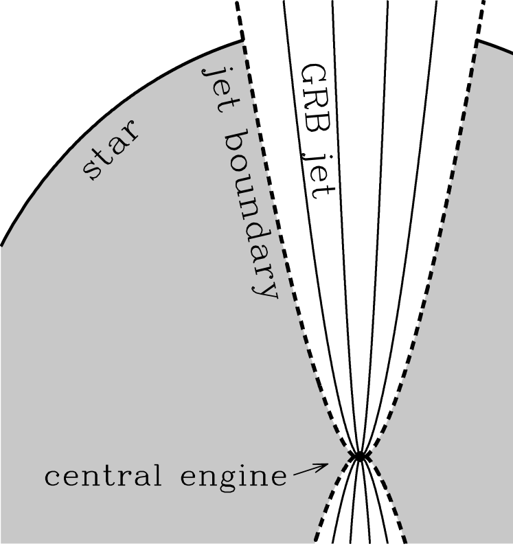
Figure 1: Cartoon of the large-scale structure of a GRB source (not to scale). The major elements are a central engine which launches a polar magnetically-dominated ultrarelativistic jet, and a gaseous stellar envelope (gray shading) which confines the jet. The central engine may be an accreting rapidly rotating black hole or a millisecond magnetar. For a failed supernova, there could also be a disc wind which may additionally confine the jet.

As depicted in Figure 1, a crucial aspect of the collapsar GRB model is that the central engine must produce a jet powerful enough to penetrate the stellar envelope. The interaction between the stellar envelope and the jet is found to be quite complex in time-dependent hydrodynamical numerical simulations of jets injected at an inlet within the presupernova core (Aloy et al., 2000; Zhang et al., 2003; Morsony et al., 2007; Wang et al., 2007). These simulations show that the jet collimates and accelerates as it pushes its way through the confining stellar envelope, thus suggesting that the envelope plays a crucial role in determining the opening angle and Lorentz factor of the flow that emerges from the star. If the collapsar system forms an accreting black hole, then the ultrarelativistic jet may be accompanied by a moderately relativistic disc wind that may provide additional collimation for the jet (McKinney, 2005b, 2006b). We note that the larger the radius of the progenitor star and/or the denser the stellar envelope, the more energy is required for the jet to have to penetrate the stellar envelope and reach the surface of the star. Burrows et al. (2007) find that a relativistic jet in the collapsar scenario may be preceded by a non-relativistic precursor jet that might clear the way for the second, relativistic jet. In the magnetar scenario, the stellar envelope is the primary collimating agent (Uzdensky & MacFadyen, 2007). Eventually, one would like to study individually the collapsar and other models of GRBs. However, at the basic level, all models are fundamentally similar, since they involve a central magnetized rotating compact object that generates a jet confined by some medium (e.g., Fig. 1).

Figure 2 shows our idealized approach to this problem. We reduce the various scenarios to a rigidly rotating star of unit radius surrounded by a razor-thin differentially rotating disc. Magnetic field lines thread both the star and the disc. We identify the field lines emerging from the star as the ‘jet’ and the lines from the disc as the ‘wind.’ Both components are treated within the magnetodynamical, or force-free, approximation. That is, they are taken to be perfectly conducting, and we assume that the plasma inertia and thermal pressure can be neglected. In terms of the standard magnetization parameter $\sigma$ (Michel, 1969; Goldreich & Julian, 1970), we assume $\sigma\rightarrow\infty$. In this idealized model, the force-free disc wind plays the role of the stellar envelope (plus any gaseous disc wind) that collimates the jet in a real GRB (Fig. 1).

In the context of the collapsar picture, the ‘wind’ region of our idealized model can be considered as a freely moving pressure boundary for the jet. The jet boundary in our simulations is able to self-adjust in response to pressure changes within the jet, and thus the boundary is able to act like the stellar envelope in a real collapsar. Notice that replacing the stellar envelope with our idealized magnetized ‘wind’ is a good approximation because in ideal MHD the wind region could be cut out (along the field line that separates the jet and wind) and replaced with an isotropic thermal gas pressure. The problem would be mathematically identical if the material in the wind region were slowly moving, as is true for the stellar envelope. Even when the material in the wind region is rapidly rotating, we show later that the pressure in the wind region changes very little, so the approximation still remains valid. Since the only importance of the wind in our model is to provide pressure support for the jet, we adjust our disc wind to match the expected properties of the confining medium in a collapsar.

We work with spherical coordinates $(r,\theta,\varphi)$, but we also frequently use cylindrical coordinates $R=r\sin\theta$, $z=r\cos\theta$. We work in the units $c=r_{0}=1$, where $c$ is the speed of light and $r_{0}$ is the radius of the compact object. Therefore, the surface of the compact object is always located at $r=1$, and the unit of time is $r_{0}/c$.

2.1 Jet Confinement

Figure 2: Idealized model studied in this paper. The thick solid lines in the upper panel show an azimuthal cut through a compact star surrounded by a razor-thin disc. The star and the disc are threaded by magnetic field lines, which are shown as thin solid lines. The magnetized plasma above the star and the disc is assumed to be perfectly conducting and to have an ultra-high magnetization parameter. Arrows show the direction of the poloidal electric current. The thick dashed line indicates the field line that separates the jet from the disc wind. The disc wind provides pressure support for the jet and plays the role of the gaseous stellar envelope in Fig. 1. The degree of pressure support is adjusted by varying the magnetic field strength profile in the disc. The lower panel shows the angular frequency of rotation of field lines as a function of the cylindrical radius of their foot-points.

Most of the jet power output from a BH accretion system moves along field lines that originate from the compact object (McKinney & Gammie, 2004; McKinney, 2006b), i.e., along the zone that we identify as the ‘jet’ in our model (Fig. 2). A crucial factor which determines the degree of acceleration and collimation of the jet is the total pressure support provided by the surrounding medium through gas pressure, magnetic pressure, ram pressure, or other forces. We parameterize the initial total confining pressure (at time $t=0$, which is the starting time of the simulation) as a power-law:

$$p_{\text{amb}}\propto r^{-\alpha}.$$ (1)

Near the compact object the accretion disc itself can provide the jet with support. For example, McKinney & Narayan (2007a, b) found via GRMHD simulations of magnetized accreting tori that the wind from their torus has an ambient pressure support that approximately follows a simple power-law with $\alpha\sim 2.5$ for two decades in radius. At a larger distance from the compact object the disc wind is expected to become less effective, and the ambient pressure in the case of a GRB is presumably due to thermal and ram pressure of the stellar envelope. According to a simple free-fall model of a collapsing star (Bethe, 1990), for which density and velocity scale as $\rho\propto r^{-3/2}$ and $v\propto r^{-1/2}$, the ram pressure varies with radius as $\sim r^{-2.5}$, identical to the GRMHD disc wind result. Moreover, hydrodynamic simulations of GRB jets show that the internal thermal pressure also has the same scaling, $\alpha\sim 2.5$ (see, e.g., Model JA-JC in Zhang et al. 2003).

In our model, the vertical component of the magnetic field at the surface of the disc is taken to vary as a power-law with radius,

$$B_{z}(R)\propto R^{\nu-2},\quad\nu=\text{const}.$$ (2)

This is our boundary condition on the field at $z=0$, $R\geq 1$. If $\nu=1$, the wind has a paraboloidal shape and the magnetic pressure has a power-law scaling $r^{-2}$, whereas if $\nu=0$, the wind corresponds to a split monopole with pressure varying as $r^{-4}$ (Blandford & Znajek, 1977; McKinney & Narayan, 2007a, b; Narayan et al., 2007). For a general value of $\nu$, the magnetic pressure in the wind is very close to a power-law, $r^{-\alpha}$, with

$$\alpha=2(2-\nu).$$ (3)

Since we wish to have $\alpha=2.5$, therefore for our fiducial model we choose

$$\nu=2-\alpha/2=0.75.$$ (4)

We have considered many other values of $\nu$, but focus on two other cases: $\nu=0.6,\;1$.

2.2 Model of the Central Compact Object

We treat the central compact object as a conductor with a uniform radial field on its surface, i.e., as a split monopole. The compact object and the field lines rotate at a fixed angular frequency $\Omega_{0}$, and it is this magnetized rotation that launches and powers the jet. We neglect all gravitational effects. As shown in McKinney & Narayan (2007a, b), this is a good approximation since (relativistic) gravitational effects do not qualitatively change the field geometry or solution of the magnetically-dominated jet even close to the BH. Also, jet acceleration is known to occur mostly at large distances from the compact object for electromagnetically-driven jets (e.g., Beskin & Nokhrina, 2006).

For a spinning BH the angular frequency of field lines in the magnetosphere is determined by general relativistic frame dragging in the vicinity of the hole. This causes the field lines threading the BH to rotate with a frequency approximately equal to half the rotation frequency of the BH horizon,

$$\Omega(a)\approx 0.5\,\Omega_{\text{H}}(a)=\frac{ac}{4r_{\text{H}}}=\frac{a}{4},$$ (5)

where the dimensionless Kerr parameter $a$ describes the BH spin and can take values between $-1$ and $1$. In our chosen units the radius of the BH horizon, $r_{\text{H}}=(1+\sqrt{1-a^{2}})GM/c^{2}$, is unity (see §2). Equation (5) is for a monopole field threading the horizon (McKinney & Narayan, 2007a, b). For field geometries other than a monopole, the field rotation frequency does not remain exactly constant on the BH horizon (Blandford & Znajek, 1977; McKinney & Narayan, 2007b). For example, for a parabolical field geometry, $\Omega$ near the poles is smaller than in the monopole case by a factor of two. We do not consider this effect in the current study. According to McKinney & Narayan (2007b) it should not change our results significantly.

Various studies of BH accretion systems suggest that rapidly spinning BHs ($a\gtrsim 0.9$) are quite common (Gammie et al., 2004; Shafee et al., 2006; McClintock et al., 2006). Therefore, for our fiducial model, we consider a maximally spinning BH with Kerr parameter $a=1$, so we choose

$$\Omega_{0}=\Omega(a=1)=0.25.$$ (6)

This is the maximum frequency that field lines threading a BH can have in a stationary solution.

Even though we primarily focus on the case of a maximally spinning BH, we also apply our model to magnetars. A magnetar with a characteristic spin period of $1$ ms and a radius of $10$ km has spin frequency $\Omega_{\text{NS}}\approx 0.21$ in the chosen units (unit of length $r_{0}=10^{6}$ cm and unit of time $r_{0}/c\approx 3.3\times 10^{-5}$ s), and so is comparable to a maximally rotating black hole. Thus, $\Omega_{0}=0.25$ is a reasonable approximation for either rapidly rotating black holes or millisecond magnetars.

2.3 Astrophysical Problem Setup: Models A, B, and C

Since we study axisymmetric magnetic field configurations, it is convenient to separate poloidal and toroidal field components,

$$\boldsymbol{B}=\boldsymbol{B}_{p}+{B}_{\varphi}\hat{\varphi}.$$ (7)

It is further convenient to introduce a magnetic field stream function $P$ to describe the axisymmetric poloidal field $\boldsymbol{B}_{p}$ (Okamoto, 1978; Thorne et al., 1986; Beskin, 1997; Narayan et al., 2007),

$$\boldsymbol{B}_{p}=\frac{1}{r^{2}\sin\theta}\frac{\partial P}{\partial\theta}\,\hat{r}-\frac{1}{r\sin\theta}\frac{\partial P}{\partial r}\,\hat{\theta}.$$ (8)

This representation automatically guarantees $\boldsymbol{\nabla}\cdot\boldsymbol{B}=0$. Here $\hat{r}$, $\hat{\theta}$, and $\hat{\varphi}$ are unit vectors in our spherical coordinate system. The stream function gives the magnetic flux $\Phi$ enclosed by a toroidal loop passing through a point $(r,\theta)$ (Narayan et al., 2007),

$$\Phi(r,\theta)=2\pi P(r,\theta).$$ (9)

We perform the simulations over the region $(1,r_{\text{max}})\times(0,\pi/2)$. We initialize the simulation with a purely poloidal initial magnetic field,

$$P=r^{\nu}(1-\cos\theta).$$ (10)

This initial field corresponds to a split monopole field configuration at the compact object (constant $\lvert B_{r}\rvert$) and has a power-law profile for the vertical component of the field on the disc. For our fiducial model A, we take $\nu=0.75$, as explained in §2.1. This magnetic field configuration has a confining pressure varying as $r^{-2.5}$ and is approximately an equilibrium nonrotating jet solution as we show in Appendix A.1.

We consider both the surface of the compact object, $r=1$, and the surface of the disc, $\theta=\pi/2$ ($z=0$), to be ideal conductors. The number of quantities we fix at these boundaries is consistent with the counting argument of Bogovalov (1997). A paraphrasing of this argument is that the number of quantities that one should relax at the boundary of a perfect conductor equals the number of waves entering the boundary. In our case of a sub-Alfvénic flow there are two waves entering the boundary: an incoming Alfvén wave and an incoming fast wave. Thus, we leave the two components of the magnetic field parallel to the conductor unconstrained, and we only set the normal component of the field.

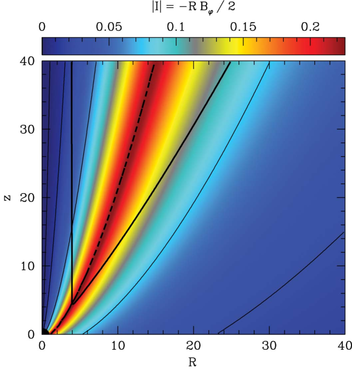
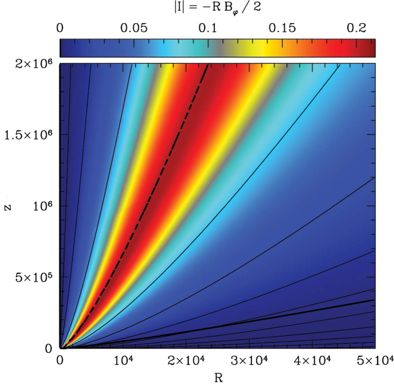
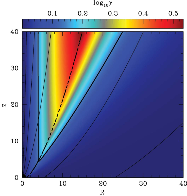
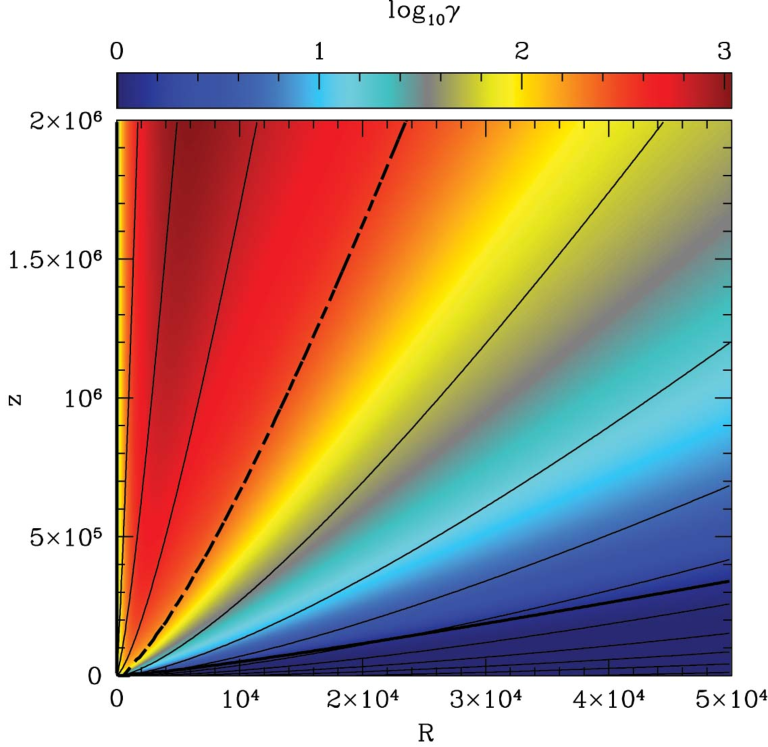
Figure 3: Poloidal magnetic field lines, shown as solid lines, overlaid on the colour-coded absolute magnitude of the enclosed poloidal current $\lvert I\rvert=\lvert RB_{\varphi}/2\rvert$ (upper panels), and the colour-coded Lorentz factor $\gamma$ (lower panels). The results are for the fiducial model A, which corresponds to $\nu=0.75$, $\Omega_{0}=0.25$, $\beta=1.5$. Left (right) panels show the near (far) region of the jet solution. The thick dashed lines indicate the position of the field line that separates the jet from the disc wind (see Fig. 2), and the thick solid lines show the position of the Alfvén surface, $\Omega R=1$. Red (blue) colour corresponds to high (low) values of the plotted quantities. Note that, for any distance from the compact object, the maximum $\lvert I\rvert$ is nearly coincident with the jet-wind boundary. However, the maximum Lorentz factor is found inside the jet, closer to the axis (see Fig. 12).

We set the values of two magnetic field drift velocity components (perpendicular to the magnetic field) through the stationarity condition (Narayan et al., 2007). For the compact object we choose a constant angular velocity rotation profile $\Omega_{0}=0.25$ (eq. 6), and for the disc we choose a Keplerian-like rotation profile,

$$\Omega^{\text{disc}}(R,z=0)=\Omega_{0}R^{-\beta},\quad\beta=3/2.$$ (11)

Where the compact object meets the disc, the magnitude of the disc angular frequency per unit Keplerian rotation frequency is $\Omega/\Omega_{K}\approx 1/2$ as consistent for millisecond magnetars of $10$ km size and mass $1.4{\rm M_{\odot}}$ and consistent with GRMHD simulations for near an $a=1$ black hole (see, e.g., McKinney & Narayan, 2007a, b). Therefore, near the compact object our model is more accurate than a precisely Keplerian model while keeping $\Omega$ everywhere continuous. We use an antisymmetric boundary condition at the polar axis $\theta=0$ and an outflow boundary condition at the outer boundary $r=r_{\text{max}}=10^{8}$. Since our time-dependent solutions never reach this artificial outer boundary, our results do not depend upon the details of the boundary condition there.

We discuss results obtained with this fiducial model A in §3.1. We also discuss two other models that differ from model A only by the value of $\nu$: model B, which has $\nu=1$ (parabolic field lines), and model C, which has $\nu=0.6$. We have run a number of other models that we mention briefly in §3.3.

2.4 Numerical Method

We use a Godunov-type scheme to numerically solve the time-dependent force-free equations of motion (McKinney, 2006a). Our code has been successfully used to model BH and neutron star magnetospheres (McKinney, 2006a, c; McKinney & Narayan, 2007a, b; Narayan et al., 2007).

To ensure accuracy and to properly resolve the jet, we use a numerical grid that approximately follows the magnetic field lines in the jet solution (Narayan et al., 2007). We are thus able to simulate the jet out to large distances without making significant errors in the solution. For the three models, A, B, C, discussed in this paper we used a resolution of $2048$x$256$. Since our grid follows the poloidal field lines, the above resolution corresponds to an effective resolution of about $2048$x$100,000$ in spherical polar coordinates. A comparison with lower-resolution runs shows that these models are well converged. In particular, over $6$ orders of magnitude in distance from the compact object, the shape of poloidal field lines is accurate to within $\delta\theta/\theta<10$% (see §3).

In order to speed up the computations, we use a time-stepping technique such that only the non-stationary region is evolved. This is achieved by defining the active section, where the evolution is performed, to be the exterior to a sphere of radius $r_{\text{stat}}=\xi_{\text{stat}}ct$, where $t$ is the time of the simulation, $c$ is the speed of light, and $\xi_{\text{stat}}=0.01$. We set the electromotive forces at all boundaries of the active section to zero. If the initial condition is a force-free solution, then this procedure is mathematically justified even within the fast critical surface since the time-dependent solution only contains outgoing waves, so the solution rapidly settles to its final state behind the wave. In all cases our initial condition is an exact solution or is close enough to the exact solution to avoid significant ingoing waves. We also experimentally verified that by not evolving the solution interior to the active section, we make an error of less than one part in ten thousand. The use of grid sectioning speeds up the simulations by a factor of up to a thousand since it allows us to use a larger time step. Komissarov et al. (2007) used a similar approach.

3 Simulation Results

We first present simulation results for our fiducial model A and analyze them morphologically. Then, we develop an analytical model of the jet structure and use it to gain insight into jet acceleration and collimation. Finally, we consider the other two jet models, B and C, and discuss the variation of jet properties with $\theta$.

3.1 Fiducial model A

Figure 4: Radial dependence of the Lorentz factor $\gamma$ in the fiducial model A for two field lines. One field line starts from the compact object at an angle $\theta_{\text{fp}}\approx 73^{\circ}$ (indicated with thick lines), and the other starts at $\theta_{\text{fp}}\approx 21^{\circ}$ (thin lines). Solid lines show the numerical solution, dashed lines show the analytical approximation (13) with $C=\sqrt{3}$ (the solid and dashed lines are virtually indistinguishable for $\theta_{\text{fp}}=21^{\circ}$), and dotted lines show the individual scalings given in (21) and (22). Note that the field line with $\theta_{\text{fp}}=73^{\circ}$ accelerates quickly as it moves away from the compact object but it then switches to a slower second regime of acceleration. In contrast, the field line with $\theta_{\text{fp}}=21^{\circ}$ begins accelerating only after it has moved a considerable distance from the compact object. However, it then maintains a rapid rate of acceleration without switching to the second acceleration regime. When the jet reaches the outer edge of the simulation at $r\sim 2\times 10^{6}$, this field line has a very large bulk Lorentz factor $\gamma>1000$, whereas the field line with $\theta_{\text{fp}}=73^{\circ}$ has a smaller $\gamma\sim 500$. Thus, the jet develops a fast core surrounded by a slower sheath.

Figure 5: Field line shape (upper panel) and comoving magnetic pressure (lower panel) in the fiducial model A for a field line that starts from the compact object at $\theta_{\text{fp}}\approx 73^{\circ}$. Solid lines show the results from the numerical simulation, and dashed lines show the analytic scalings for the non-rotating solution. Field lines with foot-points in the disc (wind) show better agreement with the analytic scalings. For example, the magnetic pressure along a field line with $r_{\text{fp}}\gtrsim 500$ (not shown) is indistinguishable from the dashed line in the lower panel.

Model A consists of a compact object of unit radius rotating with an angular frequency $\Omega_{0}=0.25$, surrounded by a Keplerian-like disc ($\beta=3/2$). On the surface of the compact object, the radial component of the magnetic field is uniform, $B_{r}=1$, while at the disc, the vertical component of the field varies with radius in a self-similar fashion with index $\nu=0.75$, i.e., $B_{z}(R,z=0)\propto R^{\nu-2}=R^{-1.25}$ (eq. 10). Starting with this purely poloidal initial field configuration, we have run the force-free simulation for a time equal to $10^{7}r_{0}/c$. At the end of the calculation we obtained a time-steady solution out to a distance of $2\times 10^{6}r_{0}$. We describe below the properties of this steady solution.

The panels in Fig. 3 show the poloidal field structure of model A in steady state. The poloidal field in the final rotating state is nearly the same as in the initial non-rotating state, just as was seen for the self-similar solutions discussed in Narayan et al. (2007). This is despite the fact the final steady solution has a strong axisymmetric toroidal field $B_{\varphi}(r,\theta)$, which is generated by the rotating boundary conditions at the star and the disc.

The toroidal field at any point is related to the total enclosed poloidal current $I(r,\theta)$ at that point by Ampere’s Law,

$$I(r,\theta)=RB_{\varphi}(r,\theta)/2\leq 0,\quad R=r\sin\theta.$$ (12)

The enclosed current is negative because we have a positive $B_{z}$ and positive $\Omega$, so that $B_{\varphi}$ is negative. The colour-coding in the upper panels of Fig. 3 indicates the absolute magnitude of the enclosed current as a function of position. As expected, we see that $I$ is constant along field lines, which corresponds to $RB_{\varphi}$ being constant. More interestingly, we see that at any $r$, the absolute value of the enclosed current starts at zero, increases as we move away from the axis, reaches a maximum value, and then decreases back to zero. The maximum in the absolute enclosed current corresponds to a transition from a negative current density (inward current) to a positive current density (outward current). This transition is coincident with the field line that originates at $r_{\rm fp}=1$, $\theta_{\rm fp}=\pi/2$ and that defines the boundary between the ‘jet’ and the ‘wind’ in our model (see Fig. 2).

As a result of rotation, the solution develops a poloidal electric field in the lab-frame (or inertial frame). The electric field strength at each point is equal to $\Omega RB_{p}$, where $\Omega$ is equal to the angular frequency at the foot-point of the local field line. The electric field gives an outward Poynting flux $\boldsymbol{S}=\boldsymbol{E}\times\boldsymbol{B}/4\pi$ which we discuss later. It also gives a drift speed $v=E/B$, and a corresponding Lorentz factor $\gamma$. The colour-coding in the lower panels of Fig. 3 indicates the variation of $\gamma$ with position in the steady solution. The Lorentz factor reaches up to a maximum $\sim 1000$ in this particular model. As Fig. 3 shows, the acceleration proceeds gradually and occurs over many decades in distance from the compact object.

Note that, at a given distance from the compact object, the maximum Lorentz factor is not achieved at either the jet-wind boundary or on the axis, but occurs at an intermediate radius inside the jet. For instance, at $z=5\times 10^{5}$, $\gamma$ is maximum at $R\sim 3\times 10^{3}$, whereas the jet-wind boundary is located at $R\sim 8\times 10^{3}$. Thus, the jet consists of a slow inner spine, fast edge, and a slow outer sheath which actually contains most of the power density. Komissarov et al. (2007) apparently observed this ‘anomalous’ effect in one of their solutions. In the next subsection we explain the origin of the effect and quantify it.

Figure 4 shows the variation of the Lorentz factor with distance along two field lines emerging from the compact object. The field line that starts closer to the equator, with $\theta_{\rm fp}=73^{\circ}$, undergoes rapid acceleration once it is beyond a distance $\sim 10$. However, at a distance $\sim 10^{3}$ it switches to a different and slower mode of acceleration, reaching a final $\gamma\sim 500$ at $r=2\times 10^{6}$. In contrast, the field line that starts closer to the axis at $\theta_{\rm fp}=21^{\circ}$ does not begin accelerating until a distance $\sim 100$. It then accelerates rapidly almost until it reaches the outer radius (there is a hint of a transition to the slower acceleration mode near the end), by which point it has a larger Lorentz factor $\sim 1000$ than the other field line. This inverted behaviour is what causes the natural development of a fast structured spine and slow sheath that contains most of the power density.

The upper panel in Figure 5 shows, for the steady state solution, the variation of polar angle $\theta$ as a function of distance along the field line that starts at $\theta_{\rm fp}=73^{\circ}$. The dashed line shows the corresponding quantity for the initial purely poloidal field with which the simulation was started. We see that the final field shape is mildly perturbed by rotation. However, even at a distance of $2\times 10^{6}$ the change in $\theta$ is no more than a factor of 2.

The lower panel in Figure 5 shows the variation of the comoving pressure with distance along the same field line. The pressure varies as $r^{-2.5}$ (the dashed line), the desired dependence, for distances up to $r\sim 10^{3}$ or so. Beyond this distance, the pressure variation in the jet becomes a little shallower. The change occurs in the region where the slower mode of acceleration operates (see Fig. 5). We explain this behaviour in the next subsection. We note that this change in pressure inside the jet does not affect the confining pressure profile of the external medium/wind which stays the same as in the initial configuration, and varies as $r^{-2.5}$.

The model A simulation described here is well-converged: the angular frequency of field line rotation $\Omega$ and the enclosed poloidal current $I$ are accurately preserved along each field line, as they should be in a stationary axisymmetric force-free solution (Mestel, 1961; Okamoto, 1978; Thorne et al., 1986; Beskin, 1997; Narayan et al., 2007). Even though the simulation domain extends over more than six decades in radius, these field-line invariants are conserved to better than $12$%, see Fig. 6.

Figure 6: Transverse variations of the field-line invariants, $\Omega$ and $\lvert I\rvert$, for model A as a function of the magnetic field stream function $P$. In each panel four curves are shown: the star-disk surface (solid line), $r=10^{2}$ (dotted), $r=10^{4}$ (short-dashed), and $r=10^{6}$ (long-dashed). Over a range of six orders of magnitude in distance, the values of $\Omega$ and $\lvert I\rvert$ are conserved to better than $12$%.

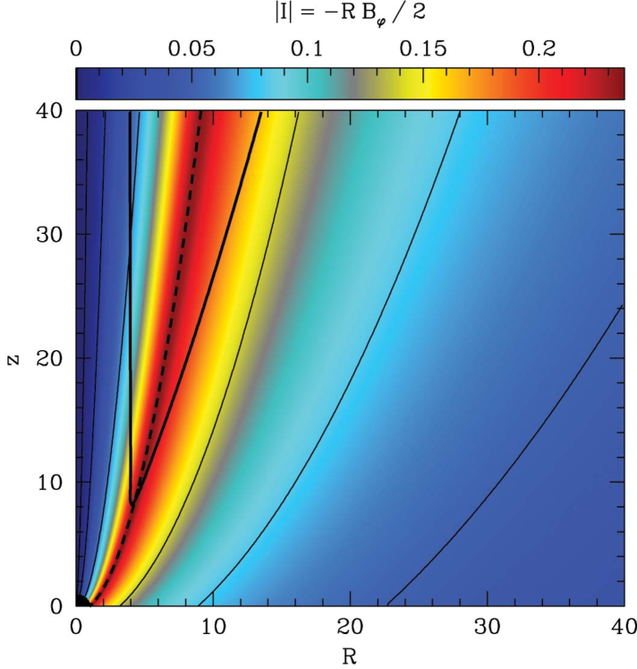
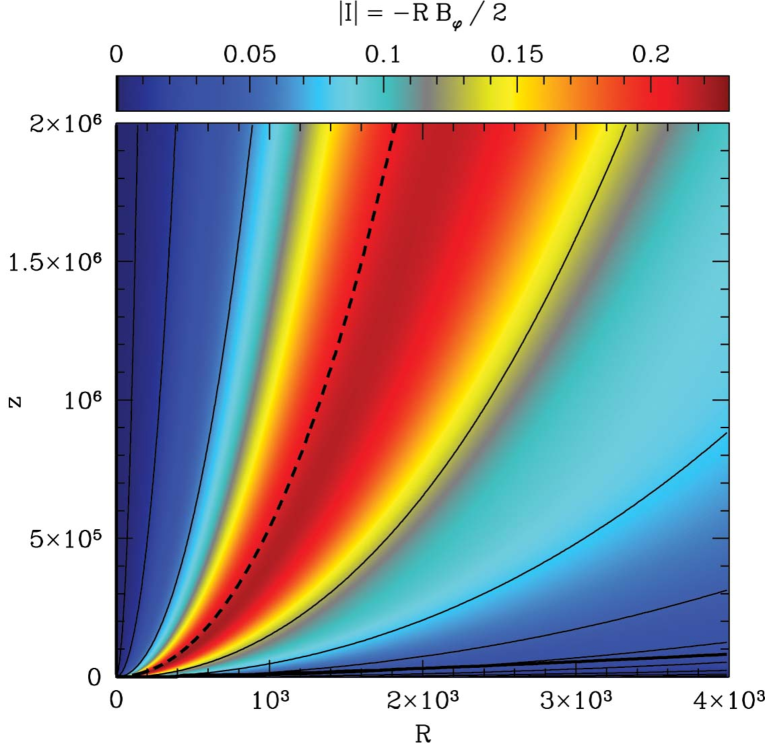
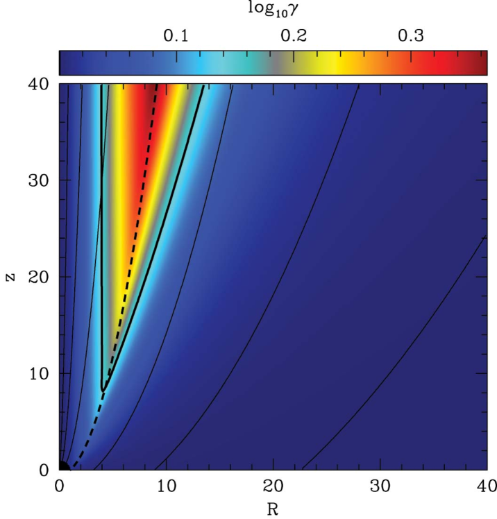
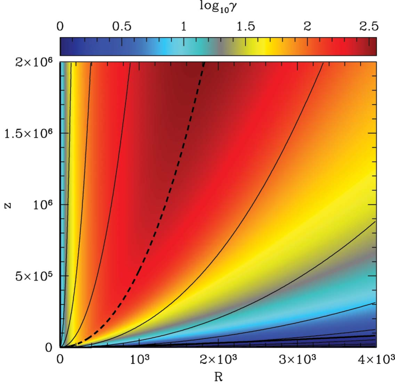
Figure 7: Similar to Fig. 3, but for model B, which corresponds to $\nu=1$, $\Omega_{0}=0.25$, $\beta=1.5$. Field lines in this model show faster collimation than in our fiducial model A. This is because the confining magnetic pressure of the disc wind falls off more slowly with distance – as $r^{-2}$ here instead of as $r^{-2.5}$ in model A. The difference in collimation is not due to hoop-stress or rotation. Note that the maximum Lorentz factor at any distance coincides with the jet-wind boundary, in contrast to what is seen in model A.

3.2 Comparison to Analytical Results

We now interpret the numerical results described above in terms of simple analytic formulae. Details may be found in the Appendix A. Here we merely summarize the relevant results.

In an axisymmetric force-free electromagnetic configuration, the drift Lorentz factor $\gamma$ can be described quite well by the following analytic formula (see Appendix A.4.1),

$$\frac{1}{\gamma^{2}}=\frac{1}{\gamma_{1}^{2}}+\frac{1}{\gamma_{2}^{2}},$$ (13)

where $\gamma_{1}$ and $\gamma_{2}$ are given by

$$\gamma_{1} \approx\left[1+(\Omega R)^{2}\right]^{1/2}\approx\Omega R,$$ (14)

$$\gamma_{2} \approx C\;\left(\frac{R_{c}}{R}\right)^{1/2},$$ (15)

where the last equality in (14) holds for $\Omega R\gg 1$. Here, $R=r\sin\theta$ is the cylindrical radius, $\Omega$ is the rotation frequency of the local field line, $R_{c}$ is the poloidal radius of curvature of the field line, and $C$ is a numerical factor of order unity that depends on the field line rotation profile (see Appendix A.7),

$$C\approx\left(3+\frac{\partial\log\Omega}{\partial\log R}\right)^{1/2}.$$ (16)

In the jet region we have $\Omega=\text{const}$ and, therefore, we expect

$$C\approx\sqrt{3}\approx 1.7.$$ (17)

As we will see in §3.3, in the simulations we find values of $C$ slightly below this value because $\Omega$ slightly decreases with increasing $R$ toward the edge of the jet (due to numerical diffusion, see Fig. 6).

Equation (13) gives the drift speed of an infinitely magnetized magnetodynamic, or force-free, flow. One might worry that the velocity of a fluid carried along with such a flow will be very different. In Appendix B we show that any such fluid has only a slightly modified Lorentz factor relative to the drift speed, in the limit when the fluid is massless, i.e., $\sigma\to\infty$. Therefore, for all practical purposes we can assume that the fluid Lorentz factor is given by eq. (13).

Since $\gamma^{2}$ is the harmonic sum of two terms, the value of $\gamma$ is determined by whichever of the two quantities, $\gamma_{1}$ and $\gamma_{2}$, is smaller. Close to the central compact star, $\gamma_{1}$ is smaller, and the first term in equation (13) dominates. Thus, for a given rotation frequency $\Omega_{0}$ of the field lines in the jet (determined by the spin of the compact object), the Lorentz factor increases linearly with distance from the jet rotation axis (Blandford & Znajek, 1977; Beskin, 1997). In this well-known regime, which we refer to as the first acceleration regime, a faster compact object spin leads to faster acceleration along the jet. Also, for a given rotation, the outermost field lines in the jet, which emerge from the equator of the star, have the largest acceleration and largest $\gamma$ at any given $z$.

The second term in equation (13) represents a slower regime of acceleration, which we refer to as the second acceleration regime. It is present only for certain field geometries and is generally realized only at large distances from the compact object. For the self-similar solutions described in Narayan et al. (2007), this acceleration regime is important only if the self-similar index $\nu<1$. Since model A has $\nu=0.75$, this term is important for our simulation. Note that models with $\nu\leq 1$ are astrophysically the most interesting and relevant (§5.1), so it is important to understand the second acceleration regime. A feature of the second acceleration regime is that the Lorentz factor does not depend explicitly on the field line rotation frequency, but is determined purely by the local poloidal curvature of the field line (Beskin et al., 2004). Moreover, as we saw earlier, the poloidal structure of the field line is itself largely independent of rotation.

Let us ignore the small distortion of the field line shape caused by rotation (Fig. 5), and take the shape to be given by the initial nonrotating solution (see Appendix A.2):

$$z\propto R^{2/(2-\nu)},\qquad\theta\propto r^{-\nu/2}.$$ (18)

The latter scaling, shown by the dashed line in Fig. 5, provides a good description of the field line shape. Using this scaling, we can evaluate $\gamma_{1}$ and $\gamma_{2}$ in the jet using equations (14) and (15) (see Appendix A.4.2),

$$\gamma_{1} \approx\Omega_{0}\,r\,\sin\theta,$$ (19)

$$\gamma_{2} \approx\kappa/\theta,$$ (20)

where $\kappa={2C}/{\sqrt{(2-\nu)\nu}}$ does not have any explicit dependence on $\Omega$ or position. This gives the following scaling of the Lorentz factor along field lines,

$$\gamma_{1} \propto r^{1-\nu/2},$$ (21)

$$\gamma_{2} \propto r^{\nu/2}.$$ (22)

Close to the central star, $\gamma_{2}$ is always larger than $\gamma_{1}$, and thus the jet $\gamma$ is determined by $\gamma_{1}$. With increasing distance along a field line, $\gamma_{1}$ and $\gamma_{2}$ grow at different rates. If $\nu>1$, $\gamma_{2}$ rises more rapidly than $\gamma_{1}$ and the Lorentz factor of the jet is always determined only by $\gamma_{1}$ (e.g., model B below, which has $\nu=1$). However, for $\nu<1$ (model A and model C), $\gamma_{2}$ rises more slowly than $\gamma_{1}$ and takes over at a certain distance from the star. This corresponds to the second slower acceleration regime seen in Fig. 4.

Figure 4 shows a comparison of the actual $\gamma$ measured in the model A simulation with the prediction from the analytic formula (13). We set $C=\sqrt{3}\approx 1.7$ (see eq. (17) and the next subsection). We find that the analytic formula for $\gamma$ agrees remarkably well with the numerical results. The formula gives the correct slopes and reproduces the distance at which the break between the two acceleration regimes occurs.

Figure 8: Similar to Fig. 4, but for model B. The analytic fit for the Lorentz factor uses the same value of $C=\sqrt{3}$ as before. Compared to model A, we see that model B lacks the second regime of acceleration. Correspondingly, there is no fast jet core present.

Figure 9: Similar to Fig. 5, but for model B. Note the excellent agreement between the numerical quantities and the analytical estimates.

As we see from Figure 4, the second regime of Lorentz factor growth is most prominent along field lines originating closer to the equator of the compact object. This is the reason for the ‘anomalous’ development of a slower-moving sheath surrounding a faster-moving structured jet spine that we mentioned in §3.1. See §3.4 for more detail.

The cause for the slight deviation of the magnetic pressure from the $r^{-2.5}$ power-law behaviour, as seen in Figure 5, is discussed in Appendix A.6. We show that, for $\nu<1$, the magnetic pressure shows a broken power-law behaviour along field lines,

$$p_{\text{mag}}\propto\begin{cases}r^{2(\nu-2)},\quad&r\lesssim r_{\text{tr}},\\ r^{-2},\quad&r\gtrsim r_{\text{tr}}.\end{cases}$$ (23)

The break radius $r_{\text{tr}}$ is the same as the radius where the jet acceleration switches from the first regime ($\gamma_{1}$) to the second ($\gamma_{2}$). The power-law indices in (23) as well as the predicted break radius $r_{\text{tr}}\approx 7\times 10^{3}$ are consistent with the results shown in Fig. 5. Note that the confining pressure of the wind (along any field line originating in the disc sufficiently far from the compact object) follows a single power-law, $r^{2(\nu-2)}$, at all distances from the compact object (see §3.1).

3.3 Dependence of the Results on Model Details

In order to explore which features of the results described above are generic and which are particular to model A, we simulated a wide range of models with $\nu$ varying from $0.5$ to $1.25$. We find that model A is representative of most models with $\nu<1$. In particular, all these models show the two regimes of Lorentz factor growth (21) and (22). Similarly, we find that model B, which has $\nu=1$ and is described below, is representative of models with $\nu\geq 1$.

Figure 10: The values of the factor $C$ as determined from simulations of jets with different choices of the field geometry threading the star, the spin of the compact object, and the rotation profile of the disc. Crosses and diamonds correspond to simulations with $\Omega_{0}=0.25$ and 0.1, respectively. The scatter is mostly due to variations of $C$ from one field line to another (see text for more detail). For $0.5\leq\nu\leq 0.8$, the numerical results lie within the expected analytical range (25), between the solid and dotted horizontal lines. For $\nu\gtrsim 0.9$ we are not able to reliably determine the value of $C$ from the simulation (an error bar is shown). However, for these values of $\nu$, the second regime of acceleration does not operate for any distance $r<10^{6}$, and the value of $C$ is unimportant. Therefore the same value of $C$ can be used here as well.

Model B has field lines with a parabolic shape, as we expect from equation (18). Figures 7, 8, and 9 show results corresponding to this model. The jet acceleration is always in the first regime and the Lorentz factor of the jet is determined only by $\gamma_{1}$. Consequently, the maximum acceleration always occurs for the field line at the jet-wind boundary. This is obvious in Fig. 7, where we see that the maximum Lorentz factor coincides with the maximum in the enclosed current. Also, in Fig. 8, we see that the Lorentz factor of the field line with $\theta_{\rm fp}=20^{\circ}$ is always smaller than that of the line with $\theta_{\rm fp}=64^{\circ}$. Our model B simulation is well-converged, with $\Omega$ and $I$ preserved along the field lines to better than $15$%, even though the simulation domain extends over six orders of magnitude in distance.

In model A, it was the presence of the second regime of Lorentz factor growth that was responsible for the development of a faster jet core. This regime is absent in model B (compare Fig. 5 and Fig. 8). Indeed, everything is much simpler in model B. For instance, Fig. 8 shows that the analytic formula for the Lorentz factor accurately reproduces the numerical profile, and Fig. 9 shows that both the field line shape and the comoving pressure accurately follow the predicted dependencies, $\theta\propto r^{-1/2}$, $p_{\rm mag}\propto r^{-2}$. We obtain this kind of close agreement for all models with $\nu\geq 1$.

We have investigated the sensitivity of the models to the rotation profile in the disc (the value of $\beta$), the magnitude of the stellar spin (the value of $\Omega_{0}$), and the geometry of the field threading the star. For $\nu$ ranging from $0.5$ to $1.25$ we tried different values of these parameters. In particular, we have done simulations with a uniform rotation velocity in the disc, i.e., $\beta=1$, which corresponds to the self-similar model of Narayan et al. (2007), and we have tried both a monopole field and a uniform vertical field threading the star. We find that these changes do not noticeably affect the jet; in particular, the field line shape changes negligibly. We have also investigated the effect of a slower stellar spin: $\Omega_{0}=0.1$. We find that the field line shape stays very close to that of the nonrotating solution so long as $\nu\geq 1$, but changes logarithmically for $\nu<1$, as in model A.

We were particularly interested to see how well the general formula for the Lorentz factor (13) performs for the range of models we considered. Since $\Omega$ in the jet region is not perfectly constant due to inevitably present numerical diffusion (Fig. 6),

$$-1\lesssim\frac{\partial\log\Omega}{\partial\log R}\lesssim 0,$$ (24)

we expect a range of values for the factor $C$ (eq. 16),

$$\sqrt{2}\lesssim C\lesssim\sqrt{3}.$$ (25)

The upper bound $C=\sqrt{3}$ (eq. 17) is the analytical value for the case $\Omega=\text{const}$. Figure 10 shows that for $0.5\leq\nu\leq 0.8$ the best-fit values of the factor $C$ for various field lines threading the star are within the expected range (25), for all models we considered. For $\nu\gtrsim 0.9$ the second regime of the Lorentz factor (15) is unimportant (it is realized if at all only at greater distances than are of interest to us), and so the value of $C$ is irrelevant. Thus, we can use the analytical value of $C$ (17) with equation (13) for all values of $\nu$ in the range $0.5\leq\nu\leq 1.25$, for all physically relevant values of $\Omega_{0}$, and for any value of $\beta$ between $1$ and $1.5$ (we have not explored other values). In all cases, for most of the jet (for field lines with $0\leq\theta_{\text{fp}}\leq 80^{\circ}$), $\Omega$ is constant to within a few percent and the Lorentz factor predicted by equation (13) agrees with the numerical results to better than $10$% (see, e.g., Figs. 4 and 8).

3.4 Collimation and Transverse Structure of Jets

Figure 11: Upper Panel: Angular dependence of the Lorentz factor $\gamma$ for the fiducial model A ($\nu=0.75$, solid lines), model B ($\nu=1$, dashed lines), and model C ($\nu=0.6$, dot-dashed lines). For each model, three distances from the compact object are shown. From bottom to top, they are $r=1.25\times 10^{5},~{}5\times 10^{5},~{}2\times 10^{6}$. For a maximally spinning BH of mass $M=3M_{\odot}$, these distances correspond to $r=6\times 10^{10}$, $2\times 10^{11}$ and $9\times 10^{11}$ cm; for a neutron star of radius $10$ km, the distances in centimeters are approximately half these values. Asterisks indicate the boundary between the jet and the wind. Note that for all models and distances shown, $\gamma$ is $\sim 100$ or larger. Note also that, for models A and C, the maximum value of $\gamma$ occurs inside the jet, whereas for model B, it occurs at the boundary between the jet and the wind. Lower Panel: Angular dependence of the jet energy flux per unit solid angle, $dP/d\omega$, for the same models and distances. The energy flux is maximum at the jet-wind boundary for all three models.

Figures 4, 5, 8, and 9 show the behaviour of various quantities along field lines in models A and B. We now consider how these quantities vary across the jet at a given distance from the compact object. The results are shown in Fig. 11.

The upper panel of Fig. 11 shows the angular profile of the Lorentz factor at various distances from the central object for each of the three models, A, B, C. Consider the simplest of the three models, model B, which has $\nu=1$. As Fig. 8 shows, in this case the Lorentz factor is simply equal to $\Omega R$ at large distances. Since the field lines in the ‘jet’ region of the outflow are all connected to the rigidly rotating compact object at the center (see Fig. 2), all of them have the same $\Omega=\Omega_{0}$. Therefore, we expect $\gamma=\Omega_{0}R\approx\Omega_{0}r\theta$. This linear increase of $\gamma$ with $\theta$ at a fixed $r$ terminates at the edge of the jet, $\theta=\theta_{j}$. At the jet boundary we have

$$\theta=\theta_{j}\approx\sqrt{\frac{2}{r}},\quad\gamma\approx{2\frac{\Omega_{0}}{\theta_{j}}}={\frac{0.5}{\theta_{j}}}\approx 0.35\sqrt{r}.$$ (26)

Beyond the edge of the jet, the field lines are attached to the disc, where $\Omega$ falls rapidly with increasing radius. Therefore, the Lorentz factor decreases quickly. Appendix A.4.2 shows that the expected dependence is $\gamma\propto\theta^{-2}$. The dashed lines in Fig. 11 confirm the scalings of $\gamma$ with $\theta$ both inside and outside the jet. They also show how $\theta_{j}$ and $\gamma$ vary with distance from the compact object.

Consider next model A, with $\nu=0.75$. Now we expect the jet angle to scale as

$$\theta_{j}\approx{\frac{\sqrt{2}}{r^{\nu/2}}}={\frac{\sqrt{2}}{r^{3/8}}}.$$ (27)

This is approximately verified in Figs. 5 and 11. However, the agreement is not perfect because field lines open out slightly at large distances relative to the analytical approximation of the field line shape.

The Lorentz factor profile has a more complicated behaviour in this model because of the presence of two different regimes of acceleration (Fig. 4). Close to the axis, the field lines are in the first acceleration regime, where $\gamma\approx\Omega_{0}R$ and the behaviour is the same as in model B, i.e. $\gamma\propto\theta$. However, at an angle $\theta=\theta_{m}$ (‘m’ for maximum), we begin to see field lines that have switched to the second acceleration regime, and beyond this point the Lorentz factor decreases with increasing $\theta$. Thus we have

$$\gamma\approx\begin{cases}\Omega_{0}r\theta,\quad&0<\theta<\theta_{m},\\ 3.8/\theta,\quad&\theta_{m}<\theta<\theta_{j}.\end{cases}$$ (28)

The coefficient 3.8 is obtained from the simulations, but it is close to the analytical value of $\kappa=3.6$. (The small difference is because of the slight opening up of the field lines in the second acceleration regime). The angle corresponding to the maximum Lorentz factor is

$$\theta_{m}\approx\sqrt{\frac{3.8}{\Omega_{0}r}}=\frac{3.9}{\sqrt{r}},$$ (29)

and the value of the maximum Lorentz factor is (eq. 13)

$$\gamma_{m}\approx\frac{1}{\sqrt{2}}\Omega_{0}r\theta_{m}\approx\sqrt{1.9\Omega_{0}r}\approx 0.7\sqrt{r}.$$ (30)

Interestingly, over the entire range of angles from $\theta_{m}$ to $\theta_{j}$, we have the simple scaling

$$\gamma=\frac{3.8}{\theta},\quad\theta_{m}<\theta<\theta_{j}.$$ (31)

Note also that the coefficient in this relation is larger than the one corresponding to model B (eq. 26). Thus, for the same Lorentz factor, the jet in model A has at least six times larger opening angle than the jet in model B. Beyond the edge of the jet, in the wind region, the Lorentz factor drops rapidly as $\theta^{-2.5}$.

We can now make a general prediction for how the peak Lorentz factor $\gamma_{m}$ scales with distance from the compact object. For a maximally spinning BH, $\gamma_{m}$ attained at a distance $r$ is likely to lie in the range bounded by models $A$ and $B$ (eqs. 26 and 30):

$$\gamma_{m}(r)=(0.3-0.7)\sqrt{r}.$$ (32)

Note that this formula gives the maximum value of the Lorentz factor over all field lines, as opposed to a value of the Lorentz factor along a single field line.

As we see from Fig. 11, model C ($\nu=0.6$) is a more extreme version of model A. The jet is significantly wider ($\theta_{j}\sim 0.2$ radians), the maximum Lorentz factor is much larger ($\sim 5000$ at $r=2\times 10^{6}$), and the maximum of $\gamma$ occurs at $\theta\ll\theta_{j}$. Unfortunately, our numerical results for this model show large deviations from the analytical model described in the Appendix. In particular, the poloidal field line shape is nearly monopolar at large distance, i.e., $\theta$ is nearly independent of $r$ along each field line, instead of behaving as $\theta\sim r^{-0.3}$ (see eq. 53). Qualitatively, however, model C is similar to model A. Model C is well-converged with $\Omega$ and $I$ preserved along the field lines to better than $15$% throughout the simulation domain.

We consider next the power output of the jet. We define the angular density of electromagnetic energy flux as

$$\frac{dP}{d\omega}=r^{2}\left\lvert\boldsymbol{S}\right\rvert=\frac{r^{2}}{4\pi}\left\lvert\boldsymbol{E}\times\boldsymbol{B}\right\rvert,$$ (33)

where $\boldsymbol{S}$ is the Poynting vector and $d\omega=d\varphi\,d\theta\sin\theta$ is the solid angle. As we show in Appendix A.8 and verify in Fig. 11, the power output grows quadratically with distance from the jet axis for all models,

$$\frac{dP}{d\omega}\approx\frac{1}{4\pi}\Omega_{0}^{2}r^{2\nu}\theta^{2},\quad\theta\leq\theta_{j},$$ (34)

reaches its maximum at the jet boundary, indicated by asterisks in Fig. 11,

$$\frac{dP}{d\omega}\biggr{|}_{\theta=\theta_{j}}\approx\frac{\Omega_{0}^{2}}{\pi\theta_{j}^{2}}\approx\frac{0.02}{\theta_{j}^{2}},$$ (35)

and falls off rapidly in the wind region as $\theta^{2-4\beta/\nu}$. Equation (35) illustrates that jets with a smaller opening angle have a larger power output per unit solid angle. The steepest decline of angular power in the wind region is $\theta^{-10}$ in model C, followed by less steep declines of $\theta^{-6}$ in model A and $\theta^{-4}$ in model B. This behaviour can be seen in the lower panel of Fig. 11. The angular power output profile in model C does not evolve with distance since the opening angle of the jet is nearly independent of distance.

The total power output in the jet and the wind is (see Appendix A.8)

$$P^{\text{jet}} \approx\frac{\Omega_{0}^{2}B_{r}^{2}}{2}=\frac{B_{r}^{2}}{32},$$ (36)

$$P^{\text{wind}} \approx\frac{\Omega_{0}^{2}B_{r}^{2}}{2(\beta/\nu-1)}=\frac{B_{r}^{2}}{32(\beta/\nu-1)},$$ (37)

where $B_{r}$ is the radial magnetic field strength near the BH. The total power is independent of the distance at which it is evaluated, which is a manifestation of the fact that energy flows along poloidal field lines. The total power output in the jet is the same for all models, and the total power in the wind varies from model to model. The most energetic wind is in model B and carries twice as much power as the jet. In model A, the wind and the jet have equal power outputs, and in model C, the power output in the wind is two thirds of the power in the jet.

To obtain the total power of the jet in physical (cgs) units, we specialize to an astrophysical system with a BH of mass $M$, radial field strength near the BH $B_{r}$, and angular rotation frequency of field lines $\Omega_{0}$. We obtain

$$P^{\text{jet}} =\frac{1}{2}\Omega_{0}^{2}\,B_{r}^{2}\,r_{0}^{2}\,c$$

$$\approx 1.8\times 10^{50}\left(\frac{\Omega_{0}}{\Omega_{\text{max}}}\right)^{2}\left(\frac{B_{r}}{10^{15}\text{G}}\right)^{2}\left(\frac{M}{3M_{\odot}}\right)^{2}\left[\frac{\text{erg}}{\text{s}}\right],$$ (38)

where $r_{0}\approx r_{g}=GM/c^{2}$ for a rapidly spinning BH. For characteristic values, $\Omega_{0}\sim\Omega_{\text{max}}=0.25c/r_{g}$, $B_{r}\sim 10^{15}$ G, $M\sim 3M_{\odot}$, and taking the typical duration of a long GRB $\sim 10-100$ s, the model predicts a total energy output of $10^{51}-10^{52}$ erg, which is comparable to the energy output inferred for GRB jets (Piran, 2005). We note that the actual value of the magnetic field $B_{r}$ might be higher since the observations only account for a fraction of the electromagnetic energy flux. Recent GRMHD simulations suggest a value of $10^{16}$ G (McKinney, 2005b).

4 Comparison to Other Work

Since the observed energy output of long GRBs is $10^{51}-10^{52}$ erg (Piran, 2005), any model of long GRBs requires a central engine capable of supplying this copious amount of energy. In the absence of magnetic fields, a possible energy source is annihilation of neutrinos from the accretion disc (Kohri et al., 2005; Chen & Beloborodov, 2007; Kawanaka & Mineshige, 2007). Attempts to include the neutrino physics self-consistently have so far not succeeded in producing relativistic jets (Nagataki et al., 2007; Takiwaki et al., 2007). However, an ad-hoc quasi-isotropic energy deposition of $10^{50}-10^{52}$ ergs into the polar regions seems to lead to jets with Lorentz factors $\sim 100$ (Aloy et al., 2000; Zhang et al., 2003, 2004; Morsony et al., 2007; Wang et al., 2007). The jets so formed are found to be stable in two and three dimensions, to accelerate via the conversion of internal energy into bulk kinetic energy, and to collimate to angles $\lesssim 5^{\circ}$ as a result of interacting with the dense stellar envelope. We note that similar hydrodynamic simulations of short GRB jets have attained much higher Lorentz factors $\sim 700$ due to the absence of a stellar envelope that the jet has to penetrate (Aloy et al., 2005).

The inclusion of magnetic fields enables the extraction of energy from spinning BHs via the Blandford-Znajek mechanism (Blandford & Znajek, 1977; Komissarov & McKinney, 2007) and from accretion discs via the action of magnetic torques (Blandford & Payne, 1982). The paradigm of electromagnetically powered jets is particularly appealing since it is able to self-consistently reproduce the observed jet energetics of long GRBs (see §3.4 and McKinney, 2005b), without any need for ad-hoc energy deposition. Numerical simulations, within the framework of general relativistic magnetohydrodynamics (GRMHD), of magnetized accretion discs around spinning BHs naturally produce mildly relativistic jets (McKinney & Gammie, 2004; McKinney, 2005b; De Villiers et al., 2005; Hawley & Krolik, 2006; Beckwith et al., 2007; Barkov & Komissarov, 2007) as well as relativistic jets with Lorentz factors $\sim 10$ (McKinney, 2006b).

Our results are consistent with those of McKinney (2006b) of a highly magnetized jet that is supported by the corona and disc wind up to a radius $r\sim\text{few}\times 10^{2}$ by which the Lorentz factor is $\sim 10$ similar to expected by our $\nu=3/4$ model. They did not include a dense stellar envelope. Beyond the distance $r\sim\text{few}\times 10^{2}$ the disk wind no longer confines the jet, which proceeds to open up and become conical as it passes the fast magnetosonic surface. Beyond the fast magnetosonic surface they find the jet is no longer efficiently accelerated, as consistent with expectations of unconfined, conical MHD solutions (Beskin et al., 1998; Bogovalov & Tsinganos, 1999). The jet simulated by McKinney (2006b) shows a mild hollow core in $\gamma$ but shows no hollow core in energy flux, although this may be a result of numerical diffusion or significant time-dependence within the jet.

Bucciantini et al. (2006, 2007, 2008); Komissarov & Barkov (2007) studied the formation and propagation of relativistic jets from neutron stars as a model for core-collapse-driven GRB jets. They were unable to study the formation and propagation of ultrarelativistic jets likely due to computational constraints and their model setup. While our model is somewhat idealized compared to those studies, we demonstrate the generic process of magnetic-driven acceleration to ultrarelativistic speeds and thus extend their simulations of magnetar-driven GRB jets.

McKinney & Narayan (2007a, b) found that the jets in their simulations are collimated by the pressure support from a surrounding ambient medium, such as a disc corona/wind or stellar envelope, rather than being self-collimated. Thus the treatment of the medium that confines the jet appears to be crucial. Komissarov et al. (2007); Barkov & Komissarov (2008) modelled the action of such an ambient medium by introducing a rigid wall at the outer boundary of the jet and studied the magnetic acceleration. They obtained solutions with Lorentz factors of $\sim 300$ with an efficient conversion of magnetic to kinetic energy. In the current work, instead of keeping the shape of the jet boundary fixed via a rigid wall, we prescribe the ambient pressure profile, so that the shape of the jet boundary can self-adjust in response to pressure changes inside the jet (McKinney & Narayan, 2007a). We believe that this is a more natural boundary condition for modeling GRB jets confined by the pressure of the stellar envelope.

The magnetodynamical, or force-free, approximation may provide a good approximation to the field geometry even in the mass-loaded MHD regime as long as the flow is far from the singular monopole case of an unconfined flow. Fendt & Ouyed (2004) used this fact to study ultrarelativistic jets in the GRB context. As in our work, they determine the field line geometry in the magnetodynamical regime, but they use energy conservation for the particles to determine an approximate MHD solution and approximate efficiency of conversion from magnetic to kinetic energy.

The conversion efficiency for fully self-consistent highly relativistic MHD solutions has been studied only for a limited number of field geometries. High conversion efficiency was found for a parabolic $\nu=1$ solution and an intermediate $\nu=2/3$ solution, but not for the singular monopole $\nu=0$ solution (Beskin et al., 1998; Beskin & Nokhrina, 2006; Barkov & Komissarov, 2008). Following this work we plan to include particle rest-mass and systematically study the efficiency of particle acceleration in highly relativistic self-consistent MHD solutions. For this we will use the same numerical scheme as in the present numerical work but optimized for the ultrarelativistic MHD regime (Gammie et al., 2003; Mignone & McKinney, 2007; Tchekhovskoy et al., 2007).

Since we assume axial symmetry in this study, our simulations cannot address the question of jet stability to the $3$D kink (screw) mode. Unlike the hydrodynamic case, we are not aware of any studies of relativistically magnetized jets in $3$D that address this issue. However, all jets in this paper have $B_{\varphi}\approx-\Omega RB_{r}$ (see eq. 80). Thus, they marginally satisfy the stability criterion of Tomimatsu et al. (2001), suggesting that our jets are marginally stable to kink instability. Also, the spontaneous development of the spine-sheath structure in models with $\nu<1$ may be naturally stabilizing (Mizuno et al., 2007; Hardee, 2007; Hardee et al., 2007).

5 Astrophysical Application

Since we consider magnetodynamic, or force-free, jets in this paper, we are not able to study the effects of mass-loading of the jet. However, we expect the main properties of our infinitely magnetized jets to carry over to mass-loaded jets, provided the latter are electromagnetically dominated. Mass-loaded jets stay electromagnetically dominated as long as the Lorentz factor is well below the initial magnetization $\sigma$ of the jet (Beskin & Nokhrina, 2006), where $\sigma$ is the ratio of electromagnetic energy flux to mass energy flux at the base of the jet. We assume that this condition is satisfied and proceed to apply our results to GRBs and other astrophysical systems with relativistic jets.

5.1 Application to Long GRBs

The first question of interest is what sets the terminal Lorentz factor of a relativistic jet. We have shown in this paper that $\gamma$ increases with distance from the compact object as $\gamma\sim 1/\theta_{j}\sim r^{\nu/2}$. The value of $\nu$ is determined by the radial dependence of the confining pressure: if pressure varies as $r^{-\alpha}\sim r^{-2.5}$, then $\nu=2-(\alpha/2)\sim 0.75$.

In the context of the collapsar or magnetar model of GRBs, the confining pressure is primarily due to the stellar envelope, and hence acceleration is expected to continue only until the jet leaves the star. Once outside, the jet loses pressure support and the magnetic field configuration will probably become conical (monopolar). This geometry is inefficient for accelerating particles to Lorentz factors larger than $\gamma_{\text{max}}\sim\sigma^{1/3}$ (Beskin et al., 1998; Bogovalov & Tsinganos, 1999). We note that mildly relativistic edges of the jet will expand quasi-spherically after the jet loses pressure support, while the ultrarelativistic jet core will open up at most conically (Lyutikov & Blandford, 2003). In fact, if the jet loses pressure support at a distance $r\sim r_{\text{s}}$ (which corresponds to the radius of the progenitor star), the opening angle of the jet core will stay approximately constant until the jet reaches a much larger distance $r\sim(\gamma\theta_{j})^{2}_{r=r_{\text{s}}}r_{\text{s}}\gtrsim 10^{2}r_{\text{s}}$ (for our models A and C). We note also that current-driven instabilities may set in when the jet loses pressure support, and much of the electromagnetic energy may be converted into thermal energy (McKinney, 2006b; Lyutikov, 2006). These additional topics are beyond the scope of the present paper and require simulations that include a loss of pressure support at large radius to model the stellar surface.

From the above discussion, we expect that the terminal Lorentz factor of the jet in a long GRB is determined primarily by the size of the progenitor star. Figure 11 shows that, for a BH of a few solar masses and stellar radii in the range ${\rm few}\times 10^{10}$ cm to $10^{12}$ cm, the Lorentz factor of the jet is expected to be between about $100$ and $5000$. Such masses and stellar radii are just what we expect for GRB progenitors, and the calculated Lorentz factors are perfectly consistent with the values of $\gamma$ inferred from GRB observations.

For our fiducial model, the size of the star determines the terminal Lorentz factor as long as the initial magnetization of the jet is sufficiently high, $\sigma\gtrsim 10^{3}$, but not infinite, $\sigma\lesssim 10^{9}$. The first condition ensures that the jet inside the star is well-described by the force-free approximation. However, once the jet breaks out of the star and its geometry becomes monopolar, the effects of finite magnetization will set in, provided the second condition is satisfied. Acceleration in such monopolar field is ineffective, therefore the growth of the Lorentz factor stops. Estimates of baryon loading of magnetized GRB jets from black hole accretion systems are somewhat uncertain. We can estimate the initial magnetization of a GRB jet as the ratio of electromagnetic jet power output (38) to the rate of baryon mass-loading of the jet (Levinson & Eichler, 2003a; McKinney, 2005a, their eq. A10), which gives a value of initial jet magnetization $\sigma\sim 10^{3}$ for characteristic values of the accretion system parameters. However, given the uncertainty in these parameters, the actual value of magnetization could be an order of magnitude lower or higher. Note that magnetically accelerated jets behave very differently from relativistic fireballs. Beyond the star fireballs adiabatically expand leading to $\gamma\propto r$ until nearly all thermal energy is exhausted, and so there is no spatial scale that sets a terminal Lorentz factor. Fireball models require the baryon-loading of the jet be fine-tuned to obtain the observed Lorentz factor and opening angle. However, in the MHD case, acceleration essentially ceases at the stellar surface for a wide range of values of $\sigma$.

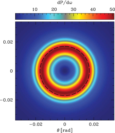
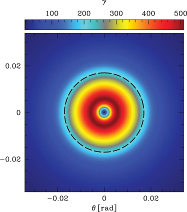
Figure 12: Face-on view of the lateral structure of the jet in model A at a distance of $r=5\times 10^{5}$ ($2\times 10^{11}$ cm for a maximally spinning BH of mass $M=3M_{\odot}$). The left panel shows the energy flux of the jet per unit solid angle, $dP/d\omega$, and the right panel shows the Lorentz factor, $\gamma$. Red colour indicates large and blue colour small values of the respective quantities. The dashed line shows the jet-wind boundary. Note that the maximum value of the energy flux, $dP/d\omega$, occurs at the jet-wind boundary, while $\gamma$ is maximal inside the jet.

We discuss next the degree of collimation of the jet. The three models we have described in this paper form a one-parameter sequence. Model B has the most highly collimated jet and model C has the least collimated jet, while our fiducial model A lies in-between. From Figure 11 we see that the models produce jet opening angles in the range $10^{-3}-0.2$ radians, which is consistent with the typical opening angles observed in long GRBs $\sim 0.03-1$ rad (Frail et al., 2001; Zeh et al., 2006). In making this comparison, we are assuming that the opening angle of the jet is set by its value when the jet emerges from the star.

Observations of GRB afterglows often indicate an achromatic ‘jet break’ in the light curve a day or two after the initial burst. These breaks suggest that the opening angle $\theta_{j}$ of the jet is substantially larger than the initial beaming angle $1/\gamma$ of the GRB. Roughly, it seems that GRBs have $\gamma\theta_{j}\gtrsim 10$. In this regard, the three models described in this paper have very different properties. Model B ($\nu=1$) has $\gamma\theta_{j}<1$. This model would predict a jet break immediately at the end of the prompt GRB, which is very different from what is seen. Model A ($\nu=0.75$) has $\gamma\theta_{j}\sim 4$ for the plasma at the boundary of the jet. This model has larger values of $\gamma$ in the interior, so it predicts a range of values of $\gamma\theta_{j}$ from $4$ up to about $15$. Model C ($\nu=0.6$) is even more extreme, giving values of $\gamma\theta_{j}\sim 25-950$. These models span a range that is more than wide enough to match observations. Our fiducial model with $\nu=0.75$ appears to be most consistent with the data.

Note that the different models correspond to different radial profiles of pressure in the confining medium: model B has pressure varying as $r^{-2}$, model A goes as $r^{-2.5}$, and model C as $r^{-2.8}$. We selected model A as our fiducial model because a superficial study of GRB progenitor star models suggested that the pressure probably varies as $r^{-2.5}$. However, in view of the fact that jet properties depend strongly on the value of the index, a more detailed study of this point is warranted.

Finally, we consider the jet power. The total energy output in a GRB jet is given by equation (38). This assumes that the power delivered by the disc wind is deposited entirely into the stellar envelope and so does not contribute to the jet, although the mass-loading of field lines near the jet-wind boundary probably depends upon the amount of turbulence in the interface (McKinney, 2006b; Morsony et al., 2007; Wang et al., 2007) and non-ideal diffusion physics (Levinson & Eichler, 2003b; McKinney, 2005a; Rossi et al., 2006). For characteristic values of the magnetic field strength $B_{r}$ near the compact object and the angular frequency $\Omega_{0}$ of the compact object, the energy released over the typical duration of a long GRB is about $10^{51}-10^{52}$ erg, which is consistent with the observed power (Piran, 2005). Other things being equal, the energy scales as $\Omega_{0}^{2}$. This scaling (Blandford & Znajek, 1977) would certainly apply to a magnetar. In the case of an accreting black hole, the magnetic field strength near the black hole may itself increase rapidly with $\Omega_{0}$ (for a fixed mass accretion rate), and this may give a steeper dependence of jet power on $\Omega_{0}$ (McKinney, 2005b).

Figure 11 indicates that the electromagnetic energy flux in the jet has a substantial variation across the jet. The power is very low near the jet axis, and most of the energy comes out near the jet boundary. Note in particular that, for the observationally relevant model A, the maximum jet power does not coincide with the maximum Lorentz factor (see Fig. 12). This unusual behaviour is the result of the second acceleration regime which we discussed in §3.4 (see Figs. 3, 4, 11). Such a ring-like shaped distribution of Lorentz factor in a fireball naturally leads to the Amati relation of an observed correlation between de-redshifted peak frequency in the GRB spectrum and the isotropic equivalent luminosity of GRBs (Eichler & Levinson, 2004). Regardless, the fact that the jet power comes out along a hollow cone, and not as a uniformly filled cone as assumed for example by Rhoads (1997, 1999) and Moderski et al. (2000), is likely to have observational consequences for both the prompt emission from a GRB and its afterglow (Granot, 2005). We are assuming, of course, that the electromagnetic power which we calculate from our model is directly proportional to the observed radiative power (both prompt and afterglow).

Rossi et al. (2002) suggested the interesting possibility that GRB jets may be ‘structured,’ with the energy flux per unit solid angle, $dP/d\omega$, having a flat core and the power falling off as $\sim\theta^{-2}$ outside the core. We have already seen that our electromagnetic jets do not have a flat core. In addition, we find that the power outside the jet, in the wind region, falls off very steeply. The variation is $\theta^{-4}$ in the mildest case (model B) and is as steep as $\theta^{-10}$ in the most extreme case (model C). In addition, the disc wind in our idealized model is merely a proxy for a gaseous confining medium, which means that the electromagnetic power in this region may be even less than we estimate. Entrainment and instabilities within the jet may lead to a less sharp distribution at large angles.

5.2 Application to AGN, X-ray Binaries, and Short GRBs

In the case of accreting black holes in active galactic nuclei (AGN), accreting neutron stars and black holes in X-ray binaries, or accreting black holes for short GRBs (which presumably form as a result of a coalescence of compact object binary systems, Piran, 2005; Meszaros, 2006), there is no stellar envelope to confine the jet. Therefore, the only confining medium available is the wind from the inner regions of the accretion disc. The strength of these winds is known to be a strong function of the radiative efficiency of the disc. A radiatively inefficient disc (i.e., an advection-dominated accretion flow, ADAF), will have a strong disc wind (Narayan & Yi, 1994), whereas a radiatively efficient disc (i.e., a standard thin disc, Shakura & Sunyaev 1973), will normally have a much weaker wind. Thus, jet acceleration should be more effective in systems with ADAFs, viz., low-luminosity AGN and black hole binaries (BHBs) in the ‘hard state’ and the ‘quiescent state’ (Narayan & McClintock, 2008). Indeed, observations indicate that these systems are invariably radio-loud, whereas higher luminosity AGN and BHBs in the ‘thermal state’, which are powered by thin accretion discs, are often radio quiet. On the other hand, some of the most energetic radio quasars are associated with high luminosity AGN which presumably have thin discs. It is unknown how such jets are confined, but large-scale force-free magnetic fields could replace the material support of the disk or wind.

The terminal Lorentz factor of the jet in an ADAF or a short GRB system will depend on the distance out to which the disc wind is able to provide significant pressure support. Numerical GRMHD simulations of ADAF-like tori of extent $r\sim 40$ around rapidly spinning BHs (McKinney, 2006b) show that the disc wind is effective to a radius $r\sim\text{few}\times 10^{2}$, giving a terminal Lorentz factor $\gamma\sim{\rm few}-10$ as long as $\sigma\lesssim 10^{3}$. Such Lorentz factors are consistent with values inferred for AGN (Jorstad et al., 2005), BHBs (Fender et al., 2004), and short GRB jets (Nakar, 2007). Under some circumstances neutron star X-ray binaries may produce jets similar to BHBs (Fender et al., 2004). Short GRBs can be mass-loaded by neutron deposition and are limited to $\sigma\lesssim 10^{3}$ just as required.

Once the confining effect of the disc wind ceases at $r\sim 100$, further acceleration will require some other confining medium, e.g., an external interstellar medium, to take over. This would appear to be unlikely for a BHB or a short GRB, but it may work for some AGN. Let us assume that the jet stops collimating (becomes monopolar) beyond $r\sim 100$. The opening angles that we expect then lie in the range bounded by the most collimated model B and the least collimated model C, $\theta_{j}\sim 0.14-0.5$ (eq. 27), i.e. substantially larger than for long GRBs. These values are perfectly consistent with the jet opening angles inferred for the systems considered in this subsection (see the above references and Watson et al., 2006).

6 Conclusions

By performing axisymmetric time-dependent numerical simulations, we have studied highly magnetized, ultrarelativistic, magnetically-driven jets. In the context of the collapsar scenario of long GRBs, we obtain global stationary solutions of magnetodynamic, or force-free, jets confined by an external medium with a radial pressure profile motivated by models of GRB progenitor stars (see §2).

We find that both the size of the progenitor star and the radial variation of pressure in the envelope of the star determine the terminal Lorentz factor and the opening angle of the jet for a wide range of initial magnetization of the jet. At the radius where the jet breaks out of the star, i.e. at a distance $r\sim 10^{10}-10^{12}$ cm, the jets in our models attain bulk Lorentz factors $\gamma\sim 100-5000$. These are currently the largest $\gamma$ attained in a numerical MHD jet simulation of long duration GRBs. The Lorentz factors we obtain are perfectly consistent with the values of $\gamma$ inferred from observations. The simulated jets have opening angles in the range $\theta_{j}\sim 10^{-3}-0.2$ radians, in agreement with the typical opening angles observed in long duration GRBs ($\sim 0.03-1$ rad, Frail et al., 2001; Zeh et al., 2006).

For a maximally rotating black hole or a $\sim 1$-ms magnetar, a characteristic magnetic field near the compact object of $10^{15}$ G, and a burst duration of $10-100$ seconds, our simulated jets provide an energy output of $10^{51}-10^{52}$ erg, comparable to the power output inferred for GRB jets (Piran, 2005).

The angular structure of the simulated jets is not uniform. The jet power comes out in a hollow cone, peaking at the jet boundary (Fig. 12). However, the Lorentz factor peaks neither at the jet axis nor at the jet boundary but rather in between (Fig. 12). This nonuniform lateral jet structure may have observational consequences for both the prompt emission from GRBs and afterglows.

To fully interpret simulation results, we derive a simple approximate analytical model (Appendix A) which gives the scaling of $\gamma$ and $\theta_{j}$ as a function of distance away from the compact object, as well as the variation of $\gamma$ and energy flux across the face of the jet. With these scalings we are able to understand all our simulation results, and we can predict the properties of highly magnetized jets in more general situations. In particular, in most of our models we find that the maximum Lorentz factor at a distance $z$ away from the compact object is $\gamma_{m}\sim(z/r_{0})^{1/2}$, where $r_{0}$ is the central black hole/magnetar radius (eq. 32).

While the magnetodynamical regime that we have studied allows us to establish the ability of highly magnetized flows to accelerate and collimate into ultrarelativistic jets, this approximation cannot be used to establish the efficiency of conversion from magnetic to kinetic energy. Following this work we plan to include particle rest-mass to study the properties of jets in the MHD regime and to determine the efficiency with which plasma is accelerated in the ultrarelativistic MHD regime. Future simulations will focus on the time-dependent formation of ultrarelativistic magnetized jets from the central engine and propagation of the jet through a realistic stellar envelope (see, e.g., Takiwaki et al. 2007; Bucciantini et al. 2008). Our present magnetodynamical and future cold MHD results should be a useful theoretical guide for understanding these more realistic and complicated simulations.

Appendix A Approximate Analytical Description of Magnetodynamic Jets

A.1 Approximate Solution for the Flux Function

An axisymmetric steady non-rotating force-free configuration is described in spherical coordinates by a magnetic flux function $P(r,\theta)$ which satisfies (Narayan et al., 2007)

$$r^{2}\frac{\partial^{2}P}{\partial r^{2}}+\sin\theta\frac{\partial}{\partial\theta}\left(\frac{1}{\sin\theta}\frac{\partial P}{\partial\theta}\right)=0.$$ (39)

Specializing to a self-similar configuration, we look for a solution of the form

$$P(r,\theta)=r^{\nu}p(\theta),$$ (40)

where we limit ourselves to $0\leq\nu\leq 2$ (Narayan et al., 2007).

Substituting (40) into (39), we obtain the following differential equation for $p(\theta)$,

$$p^{\prime\prime}(\theta)-\cot\theta\,p^{\prime}(\theta)+\nu(\nu-1)p(\theta)=0,$$ (41)

with boundary conditions, $p(0)=0$ and $p(\pi/2)=1$. The general solution is

$$p(\theta)=c_{1}f_{1}(\theta)-c_{2}\cos\theta f_{2}(\theta),$$ (42)

where $f_{1}$ and $f_{2}$ are hypergeometric functions,

$$f_{1}(\theta) ={}_{2}F_{1}\!\!\left(\frac{\nu}{2}-\frac{1}{2},-\frac{\nu}{2};\frac{1}{2};\cos^{2}\theta\right),$$ (43)

$$f_{2}(\theta) ={}_{2}F_{1}\!\!\left(\frac{1}{2}-\frac{\nu}{2},\frac{\nu}{2};\frac{3}{2};\cos^{2}\theta\right),$$ (44)

and the constants $c_{1}$ and $c_{2}$ are determined from the boundary conditions,

$$c_{1}=1,\quad c_{2}=\frac{\nu\Gamma\left(3/2-\nu/2\right)\Gamma\left(\nu/2\right)}{\Gamma\left(1-\nu/2\right)\Gamma\left(\nu/2+1/2\right)}.$$ (45)

For the particular cases of $\nu=1$ and $\nu=0$, we find that $f_{1}(\theta)\equiv f_{2}(\theta)\equiv 1$, and the solution is very simple: $p(\theta)=1-\cos\theta$. Using this result as a guide, we write down the following approximate solution for the general case:

$$P(r,\theta)\approx r^{\nu}(1-\cos\theta).$$ (46)

This turns out to be a good approximation to the exact solution for $0\leq\nu\leq 1.25$. The relative error in $P$ is less than 10% over this entire range of $\nu$.

The most attractive feature of (46) is its simplicity. Furthermore, although we began by considering a non-rotating configuration, the same solution turns out to be a reasonable approximation even for the rotating case, at least for rotations up to the maximum we consider, $\Omega_{\rm max}=0.25$. Thus, using (46), we can obtain a variety of useful, though approximate, results to describe force-free jets.

A.2 Field Line Shape

By definition, the flux function $P(r,\theta)$ is constant along a field line. Therefore, it is straightforward to obtain from equation (46) the shape of a field line as a function of the position of its footpoint, $r=r_{\text{fp}}$, $\theta=\theta_{\text{fp}}$:

$$1-\cos\theta=\left(\frac{r}{r_{\text{fp}}}\right)^{-\nu}(1-\cos\theta_{\text{fp}}),$$ (47)

which can be rewritten as

$$\sin\frac{\theta}{2}=\left(\frac{r}{r_{\text{fp}}}\right)^{-\nu/2}\sin\frac{\theta_{\text{fp}}}{2}.$$ (48)

We are primarily interested in the properties of the jet at large distances from the compact object, where field lines collimate and $\theta\ll 1$. In this limit, the field line shape is given by

$$\theta \approx\left(\frac{r}{r_{\text{fp}}}\right)^{-\nu/2}2\sin\frac{\theta_{\text{fp}}}{2},$$ (49)

or, inverting the formula,

$$\frac{r}{r_{\text{fp}}} \approx\theta^{-2/\nu}\left(2\sin\frac{\theta_{\text{fp}}}{2}\right)^{2/\nu}.$$ (50)

In cylindrical coordinates, the field line shape is

$$\frac{R}{r_{\text{fp}}} \approx\left(\frac{z}{r_{\text{fp}}}\right)^{1-\nu/2}2\sin\frac{\theta_{\text{fp}}}{2},$$ (51)

$$\frac{z}{r_{\text{fp}}} \approx\left(\frac{R}{r_{\text{fp}}}\right)^{2/(2-\nu)}\left[2\sin\frac{\theta_{\text{fp}}}{2}\right]^{-2/(2-\nu)}.$$ (52)

In the models we analyzed in the main text of the paper, we defined the ‘jet’ to include all field lines whose footpoints are on the compact central object, $r_{\text{fp}}=1$, $0\leq\theta_{\text{fp}}<\pi/2$, and the ‘wind’ to consist of the remaining field lines with footpoints on the disc, $r_{\text{fp}}>1,\theta_{\text{fp}}=\pi/2$. Thus, the field line that emerges at $r_{\text{fp}}=1$, $\theta_{\text{fp}}=\pi/2$ defines the boundary between the jet and the wind. The angle $\theta_{j}$ of this field line at a distance $r$ is

$$\theta_{j}\approx\sqrt{2}r^{-\nu/2}.$$ (53)

This relation shows how collimation proceeds as a function of distance for a given value of $\nu$. Since the models of interest to us have $0.5<\nu<1$, the collimation is gradual, going more slowly than $1/\sqrt{r}$.

Field lines with $\theta<\theta_{j}$ connect back to the central object ($r_{\text{fp}}=1$), and their foot-points are located at

$$r_{\text{fp}}=1,~{}\sin{\frac{\theta_{\text{fp}}}{2}}\approx\frac{1}{\sqrt{2}}\frac{\theta}{\theta_{j}},\quad 0\leq\theta\leq\theta_{j}.$$ (54)

Field lines at larger angles connect back to the disc ($\theta_{\text{fp}}=\pi/2$), and their foot-point radii are given by

$$r_{\text{fp}}\approx\left(\frac{\theta}{\theta_{j}}\right)^{2/\nu},~{}\theta_{\text{fp}}=\pi/2,\quad\theta_{j}<\theta.$$ (55)

A.3 Poloidal Magnetic Field

Given the magnetic flux function (46), we can determine the poloidal components of the magnetic field according to (8),

$$B_{r} =r^{\nu-2},$$ (56)

$$B_{\theta} =-\nu r^{\nu-2}\tan(\theta/2).$$ (57)

Both components of the field vary with radius as $r^{\nu-2}$, as they should for the assumed form of $P(r,\theta)$. Moreover, $B_{r}$ does not vary with $\theta$, which is approximately the case for self-similar force-free models (Narayan et al., 2007). In the context of our problem, we see that the normal component of the field at the surface of the central compact object ($r=1$) is independent of $\theta$. Thus we have a uniform field emerging from the object — a split monopole. This is a nice property of the flux function (46).

For reference, we provide the poloidal components of the magnetic field in cylindrical coordinates,

$$B_{R} =B_{r}\sin\theta+B_{\theta}\cos\theta=r^{\nu-2}[1+(1-\nu)\cos\theta]\tan{\frac{\theta}{2}},$$

$$B_{z} =B_{r}\cos\theta-B_{\theta}\sin\theta=r^{\nu-2}[\cos\theta+\nu\sin\theta\tan{\frac{\theta}{2}}],$$

In the disc plane ($\theta=\pi/2$), we have

$$B_{R} =\phantom{\nu}r^{\nu-2}=B_{r},$$ (58)

$$B_{z} =\nu r^{\nu-2}=-B_{\theta}.$$ (59)

The normal component of the field on the disc varies as a power-law in radius.

A.4 Lorentz Factor

A.4.1 General Formula for the Lorentz Factor

For an axisymmetric configuration in steady state, the angular velocity $\Omega$ is constant on field lines. This means that the comoving frame of the fluid at any position rotates at the same $\Omega$ as the angular velocity of the disc at the corresponding footpoint. In this rotating frame, there is no electric field (since we assume infinite conductivity). Therefore, in the inertial/lab frame, the electric field $\boldsymbol{E}$ is perpendicular to the magnetic field $\boldsymbol{B}$ and is equal to (Thorne et al., 1986; Beskin, 1997; Narayan et al., 2007)

$$E=\Omega RB_{p},$$ (60)

where $B_{p}$ is the magnitude of the poloidal magnetic field.

In the force-free approximation, the velocity of the fluid may be conveniently taken to be the drift velocity (Narayan et al., 2007),

$$v_{d}=\left\lvert\frac{\boldsymbol{E}\times\boldsymbol{B}}{B^{2}}\right\rvert=\frac{E}{B}.$$ (61)

This gives the Lorentz factor $\gamma$ of the fluid,

$$\frac{1}{\gamma^{2}}=\frac{B^{2}-E^{2}}{B^{2}}=\frac{B_{p}^{2}}{B^{2}}+\frac{B_{\varphi}^{2}-E^{2}}{B^{2}}.$$ (62)

Consider now the far asymptotic region of the jet where $\Omega R\gg 1$ and the velocity is ultrarelativistic, $v^{2}\approx 1$, $\gamma\gg 1$. In this limit we have $E\gg B_{p}$ due to (60) and $E\approx B$ due to (61). These two relations, combined with the definition (7) of $B$ in terms of $B_{p}$ and $B_{\varphi}$, allow us to obtain the relative magnitudes of the electromagnetic field components,

$$B\approx\lvert B_{\varphi}\rvert\approx E\gg B_{p}\quad\text{for}\quad\Omega R\gg 1,\;v^{2}\approx 1.$$ (63)

At small distances from the compact object the first term on the r.h.s. of (62) dominates, and we write its inverse as

$$\frac{B^{2}}{B_{p}^{2}}=1+\frac{B_{\varphi}^{2}}{B_{p}^{2}}=\gamma_{1}^{2},$$ (64)

where from (60) and (63) we have

$$\gamma_{1}\approx\left[1+(\Omega R)^{2}\right]^{1/2},$$ (65)

In this near-zone, we have $\gamma\approx\gamma_{1}\approx\Omega R$. We refer to this as the first acceleration regime. Formula (65), as we will see below, gives a good approximation to the Lorentz factor at moderate distances from the compact object and has been noted by many authors (Blandford & Znajek, 1977; Beskin et al., 1998; Beskin & Nokhrina, 2006; Narayan et al., 2007).

For certain field geometries it is the second term on the r.h.s. of (62) that determines the bulk Lorentz factor. The inverse of the second term can be written as

$$\frac{B^{2}}{B_{\varphi}^{2}-E^{2}}=\gamma_{2}^{2},$$ (66)

where $\gamma_{2}$ is determined by the ratio of the local poloidal radius of curvature of the field line $R_{c}$ to the cylindrical radius from the jet axis $R$ (Beskin et al., 2004, and §A.7),

$$\gamma_{2}\approx C\;\left(\frac{R_{c}}{R}\right)^{1/2}.$$ (67)

Here $C$ is a numerical factor of order unity which has to be determined by a more careful study of the solution. The value of this factor depends on the spatial distribution of field line rotation frequency $\Omega$ and as we show analytically in Appendix A.7, in the jet region, where $\Omega=\text{const}$, we have $C=\sqrt{3}\approx 1.73$. We find that this single value of $C$ does a very good job of explaining all our numerical results, giving an error of less than $10$% in all cases we have considered (see §3). Equation (67) corresponds to the second acceleration regime. It illustrates that, in a relativistic electromagnetic flow, collimation and acceleration are suppressed: for the fluid to have a sufficiently large Lorentz factor, the field line to which it is attached has to be sufficiently straight, i.e. have a sufficiently large value of $R_{c}/R$.

Combining equations (62) – (67) we obtain the following general formula for the Lorentz factor,

$$\frac{1}{\gamma^{2}}=\frac{1}{\gamma_{1}^{2}}+\frac{1}{\gamma_{2}^{2}},$$ (68)

where $\gamma_{1}$ and $\gamma_{2}$ are given by (65) and (67). Although we derived this expression in the asymptotic limit of large Lorentz factors, the formula is quite accurate all the way from the foot-point of field lines to large distances (see §3).

A.4.2 Lorentz Factor of the Jet and the Wind

In order to numerically evaluate formula (68) for our jet-wind solution, we adopt the field line shape (49). In the jet all field lines rotate at the same frequency,

$$\Omega^{\text{jet}}=\Omega_{0}=\text{const},$$ (69)

whereas in the wind field lines rotate differentially, according to the rotation profile in the disc,

$$\Omega^{\text{wind}}(r,\theta)=\Omega[r_{\text{fp}}(r,\theta)]\approx\Omega_{0}(r^{\nu}\theta^{2}/2)^{-\beta/\nu}.$$ (70)

We have used (55) to substitute for $r_{\text{fp}}(r,\theta)$ and equation (11) to substitute for $\Omega(R_{\text{fp}})$. Combining expressions (69) and (70) we have

$$\Omega(r,\theta)\approx\begin{cases}\Omega_{0},&\theta\leq\theta_{j}\quad\text{(jet)},\\ \Omega_{0}(r^{\nu}\theta^{2}/2)^{-\beta/\nu},&\theta>\theta_{j}\quad\text{(wind)}.\end{cases}$$ (71)

The first acceleration regime is straightforward. For both the jet and the wind we have

$$\gamma_{1}=\Omega(r,\theta)\,r\,\theta.$$ (72)

For the second acceleration regime, we use the asymptotic field line shape (51) to compute the curvature radius of the field line,

$$R_{c}=\frac{\left[1+(dR/dz)^{2}\right]^{3/2}}{\left\lvert d^{2}R/dz^{2}\right\rvert}\approx\frac{1}{\left\lvert d^{2}R/dz^{2}\right\rvert},$$ (73)

which together with the field line shape (51) gives

$$\frac{R_{c}}{r_{\text{fp}}}\approx\left(\frac{z}{r_{\text{fp}}}\right)^{1+\nu/2}\times\frac{1}{(1-\nu/2)\nu\sin(\theta_{\text{fp}}/2)}.$$ (74)

Therefore, according to (51) and (67), for the jet field lines we have

$$\gamma_{2}\approx\frac{1}{\theta}\times\frac{2C}{\sqrt{(2-\nu)\nu}}.$$ (75)

Note that the only explicit dependence of the Lorentz factor on position in the second acceleration regime is the spherical polar angle. Even though this expression rather accurately describes the distribution of the Lorentz factor in the jet with one single value of $C=\sqrt{3}$ (§3.3), we find that in the wind the values of $C$ are different for different field lines because in the wind the field line shape deviates from the analytical expectation (51).

A.4.3 Lorentz Factor Scaling Along Field Lines

Consider a field line starting at a foot-point $r=r_{\text{fp}}$, $\theta=\theta_{\text{fp}}$, and rotating at a frequency $\Omega_{\text{fp}}$. For a jet field line we have $r_{\text{fp}}=1$ whereas for a wind field line we have $\theta_{\text{fp}}=\pi/2$. Let us evaluate the Lorentz factor scalings (65) and (67) along a given field line as a function of distance from the compact object. Using various results derived earlier we obtain

$$\gamma_{1} \approx\Omega_{\text{fp}}\,r_{\text{fp}}\left(\frac{r}{r_{\text{fp}}}\right)^{1-\nu/2}\times 2\sin\frac{\theta_{\text{fp}}}{2},$$ (76)

$$\gamma_{2} \approx C\left(\frac{r}{r_{\text{fp}}}\right)^{\nu/2}\times\left[\sqrt{(2-\nu)\nu}\,\sin\frac{\theta_{\text{fp}}}{2}\right]^{-1}.$$ (77)

Since $C=\sqrt{3}$ and $\Omega_{\text{fp}}$ is substantially less than unity, it is easy to see that at small radii we have $\gamma_{1}<\gamma_{2}$. By equation (68), $\gamma$ is determined by the smaller of $\gamma_{1}$ and $\gamma_{2}$. Therefore, near the base of each field line the fluid is always in the first acceleration regime. As the field line goes to larger distances, $\gamma_{1}$ and $\gamma_{2}$ increase at different rates. If $\nu\geq 1$, $\gamma_{1}$ always remains smaller than $\gamma_{2}$, and the first acceleration regime operates throughout the field line. However, for $\nu<1$, $\gamma_{2}$ grows more slowly than $\gamma_{1}$. At a certain distance along the field line, $\gamma_{2}$ then becomes smaller than $\gamma_{1}$ and the flow makes a transition to the second acceleration regime (Narayan et al., 2007). The transition between the two regimes happens at a distance $r_{\rm tr}$ given by

$$\frac{r_{\text{tr}}}{r_{\text{fp}}}=\left[\frac{1}{\Omega_{\text{fp}}r_{\text{fp}}}\times\frac{C}{2\sin^{2}(\theta_{\text{fp}}/2)\sqrt{(2-\nu)\nu}}\right]^{1/(1-\nu)}.$$ (78)

Equation (78) shows that the transition occurs sooner for field lines with foot-points at lower latitudes ($\theta_{\text{fp}}$ closer to $\pi/2$) on the compact object compared to field lines that emerge near the pole. This leads to the development of a fast jet core in the polar region, where the Lorentz factor continues to be determined by the first acceleration regime for a long distance, surrounded by a slower sheath, where the acceleration switches to the second less-efficient regime at a shorter distance (see §3).

A.5 Toroidal Magnetic Field and Enclosed Poloidal Current

To obtain the toroidal magnetic field $B_{\varphi}$, we use the fact that in ideal MHD the enclosed poloidal current,

$$I=RB_{\varphi}/2,$$ (79)

is constant along each field line (Thorne et al., 1986; Beskin, 1997; Narayan et al., 2007). A positive value of $I$ indicates a current in the positive $z$ direction.

Asymptotically far from the compact object, where the fluid motion is ultrarelativistic ($\gamma\gg 1$), we have according to (63),

$$B_{\varphi}\approx-\Omega RB_{p},$$ (80)

where the negative sign is because the field lines are swept back in the opposite direction to rotation, i.e. in the negative $\varphi$-direction for a positive $\Omega$. Since asymptotically, $\theta\ll 1$, according to (56) – (57) we have $B_{p}\approx B_{r}=r^{\nu-2}$ and therefore

$$I=-\Omega R^{2}r^{\nu-2}/2\approx-\Omega\,(r^{\nu}\theta^{2}/2),$$ (81)

where we have approximated $R\approx r\theta$. According to (46), the expression in parentheses is approximately equal to the flux function $P$. Therefore we have

$$I\approx-\Omega P.$$ (82)

This relation between two quantities that are each conserved along field lines must hold throughout the solution (although we derived it only asymptotically). Therefore, according to (79) and (82), we obtain

$$B_{\varphi}\approx-\frac{2\Omega P}{R}=-\frac{2\Omega r^{\nu}(1-\cos\theta)}{r\sin\theta}=-2\Omega r^{\nu-1}\tan\left(\frac{\theta}{2}\right).$$ (83)

A.6 Magnetic Pressure

Because of the assumption of perfect conductivity, the electric field in the comoving frame of the fluid vanishes and there is only a comoving magnetic field $b$. Given the electric and magnetic fields in the lab frame, $E$ and $B$, the comoving magnetic field strength is

$$b=\sqrt{B^{2}-E^{2}},$$ (84)

and the comoving magnetic pressure is

$$p_{\text{mag}}=\frac{b^{2}}{8\pi}.$$ (85)

From (84), we can write

$$b^{2}=B_{p}^{2}+B_{\varphi}^{2}-E^{2}\approx B_{p}^{2}+\frac{B^{2}}{\gamma_{2}^{2}},$$ (86)

where the approximate equality is due to (66). Further, due to (63) and (65), we can rewrite (85) as

$$p_{\text{mag}}=\frac{b^{2}}{8\pi}\approx\frac{B_{p}^{2}}{8\pi}\left(1+\frac{\gamma_{1}^{2}}{\gamma_{2}^{2}}\right),$$ (87)

where $B_{p}^{2}/(8\pi)$ is the pressure that the jet would have if the compact object was not spinning (when $B_{\varphi}=E=0$).

If $\nu\geq 1$, we saw earlier that we always have $\gamma_{1}<\gamma_{2}$. Therefore, using the expression for the radial magnetic field (56), we obtain

$$\nu\geq 1:\qquad p_{\text{mag}}\propto r^{2(\nu-2)}.$$ (88)

The magnetic pressure follows a single power-law. However, for $$\nu<1 \gamma_{1} \gamma_{2} r_{\text{tr}}$$, the term involving the Lorentz factors in (86) cannot be neglected. Using the expressions for  (76),  (77) and the transition radius  (78), we obtain

$$p_{\text{mag}}\propto r^{2(\nu-2)}\left[1+\left(\frac{r}{r_{\text{tr}}}\right)^{2(1-\nu)}\right],$$ (89)

and the magnetic pressure behaves as a broken power-law,

$$\nu<1:\qquad p_{\text{mag}}\propto\begin{cases}r^{2(\nu-2)},\quad&r\lesssim r_{\text{tr}},\\ r^{-2},\quad&r\gtrsim r_{\text{tr}}.\end{cases}$$ (90)

Note that the power-law index at large distances is independent of the value of $\nu$.

A.7 Transverse Force Balance

In this section we study the steady state transversal force balance in force-free jets and analytically determine the value of the prefactor $C$ that scales the Lorentz factor in the second acceleration regime (eq. 67). The force balance equation is

$$\boldsymbol{j}\times\boldsymbol{B}+\rho\boldsymbol{E}=0,$$ (91)

where $\rho$ and $\boldsymbol{j}$ are the lab-frame electric charge and current density. Using Ampere’s law,

$$\boldsymbol{j}=\frac{1}{4\pi}\boldsymbol{\nabla}\times\boldsymbol{B},$$ (92)

we have

$$4\pi\boldsymbol{j}\times\boldsymbol{B}=(\boldsymbol{\nabla}\times\boldsymbol{B})\times\boldsymbol{B}=(\boldsymbol{B}\boldsymbol{\nabla})\boldsymbol{B}-\frac{1}{2}\boldsymbol{\nabla}(B^{2}).$$ (93)

Let us introduce a local orthonormal tetrad

$$({{\hat{\tau}}}=\boldsymbol{B}_{p}/B_{p},{{\hat{\varphi}}},{{\hat{n}}}=\boldsymbol{E}/E),$$ (94)

corresponding to local rotated cylindrical coordinates,

$$(\tau,R\varphi,n),$$ (95)

where $\tau$ measures the distance along field lines, $n$ measures distance perpendicular to field lines, and $R\varphi$ measures the distance in the toroidal direction. We have then

$$(\boldsymbol{B}\boldsymbol{\nabla})\boldsymbol{B}=(B_{\tau}\frac{\partial}{\partial\tau}+B_{\varphi}\frac{\partial}{R\partial\varphi}+B_{n}\frac{\partial}{\partial n})(B_{\tau}{{\hat{\tau}}}+B_{\varphi}{{\hat{\varphi}}}+B_{n}{{\hat{n}}}).$$

Projecting the above relation along ${{\hat{n}}}$, we obtain:

$${{\hat{n}}}\cdot\left[(\boldsymbol{B}\boldsymbol{\nabla})\boldsymbol{B}\right] ={{\hat{n}}}\cdot B_{\tau}\frac{\partial}{\partial\tau}(B_{\tau}{{\hat{\tau}}})+{{\hat{n}}}\cdot B_{\varphi}\frac{\partial}{R\partial\varphi}(B_{\varphi}{{\hat{\varphi}}})$$

$$=B_{\tau}^{2}\,\left({{\hat{n}}}\cdot\frac{\partial{{\hat{\tau}}}}{\partial\tau}\right)+B_{\varphi}^{2}\,\left({{\hat{n}}}\cdot\frac{\partial{{\hat{\varphi}}}}{R\partial\varphi}\right)$$

$$=\frac{B_{\tau}^{2}}{R_{c}}-\frac{B_{\varphi}^{2}}{R}({{\hat{n}}}\cdot\hat{R}),$$ (96)

where $\hat{R}$ is a unit vector directed along the cylindrical radius. Combining the above results, we have for the force balance in the ${{\hat{n}}}$-direction:

$$\frac{B_{p}^{2}}{4\pi R_{c}}-\frac{B_{\varphi}^{2}}{4\pi R}({{\hat{n}}}\cdot\hat{R})-\frac{\partial}{\partial n}\left(\frac{B^{2}}{8\pi}\right)+\frac{(\boldsymbol{\nabla}\cdot\boldsymbol{E})}{4\pi}E=0.$$ (97)

We can write the divergence of the electric field in the local rotated cylindrical coordinates as

$$\boldsymbol{\nabla}\cdot\boldsymbol{E} =\frac{1}{R}\frac{\partial}{\partial\tau}(RE_{\tau})+\frac{1}{R}\frac{\partial}{\partial n}(RE_{n})$$

$$=\frac{\partial E_{\tau}}{\partial\tau}+\frac{1}{R}\frac{\partial R}{\partial n}E_{n}+\frac{\partial E_{n}}{\partial n},$$ (98)

where we have used the fact that $E_{\tau}=E_{\varphi}=0$. The first term in (98) can be rewritten in terms of the curvature radius of the field line:

$$\frac{\partial E_{\tau}}{\partial\tau}={{\hat{\tau}}}\cdot\frac{\partial(E{{\hat{n}}})}{\partial\tau}=E\,\left({{\hat{\tau}}}\cdot\frac{\partial{{\hat{n}}}}{\partial\tau}\right)=-\frac{E}{R_{c}}.$$ (99)

Finally, combining equations (97) – (99), we obtain a form of the force balance equation that does not explicitly contain any derivatives along field lines:

$$\frac{B_{p}^{2}-E^{2}}{4\pi R_{c}}-(\hat{R}\cdot{{\hat{n}}})\frac{B_{\varphi}^{2}-E^{2}}{4\pi R}-\frac{\partial}{\partial{{\hat{n}}}}\left(\frac{B^{2}-E^{2}}{8\pi}\right)=0.$$ (100)

This equation is the analog of equation (79) in Beskin & Nokhrina (2006, they have a sign typo).

At large distances from the compact object we have $(\hat{R}\cdot{{\hat{n}}})\approx-1$ and $\partial/\partial{{\hat{n}}}\approx-\partial/\partial R$ (eq. 51). With this we can re-write (100) in projection along $\hat{R}$,

$$-\frac{B_{p}^{2}-E^{2}}{4\pi R_{c}}-\frac{B_{\varphi}^{2}-E^{2}}{4\pi R}-\frac{\partial}{\partial R}\left(\frac{B_{p}^{2}+B_{\varphi}^{2}-E^{2}}{8\pi}\right)\approx 0.$$ (101)

This form explicitly shows that the poloidal and toroidal relativistic hoop stresses, which are the first two terms, are balanced by the comoving pressure gradient, the last term.

Assuming that the field line rotation frequency varies as a power-law in the cylindrical radius, $\Omega\propto R^{\lambda}$, we have $B_{\varphi}\approx-\Omega RB_{p}\propto R^{1+\lambda}$ (eq. 63), where we took $B_{p}$ to be nearly independent of $R$ (eq. 56 – 57). With the help of (66) we have,

$$B_{\varphi}^{2}-E^{2}\approx\frac{B_{\varphi}^{2}}{\gamma_{2}^{2}}\propto R^{4+2\lambda},$$ (102)

where we used eq. (75) for the Lorentz factor in the second acceleration regime, which gives $\gamma_{2}\propto 1/R$. We note that in the wind the poloidal magnetic field is not uniform, and $\gamma_{2}$ follows a different power-law.

In the second acceleration regime we have $\gamma_{1}\gg\gamma_{2}$ and thus $B_{\varphi}^{2}-E^{2}\gg B_{p}^{2}$ (Appendix A.4.1). Therefore in this limit the terms involving $B_{p}$ in (101) can be dropped,

$$\frac{B_{\varphi}^{2}-E^{2}}{R}+\frac{\partial}{\partial R}\left(\frac{B_{\varphi}^{2}-E^{2}}{2}\right)\approx\frac{E^{2}}{R_{c}}.$$ (103)

By combining equations (102) and (103) with (63) and (66), we can express the Lorentz factor in the second acceleration regime as

$$\gamma_{2}\approx\left(\frac{E^{2}}{B_{\varphi}^{2}-E^{2}}\right)^{1/2}\approx C\left(\frac{R_{c}}{R}\right)^{1/2},$$ (104)

where

$$C=\sqrt{3+\lambda},\quad\lambda=\frac{\partial\log\Omega}{\partial\log R}.$$ (105)

Specializing to the jet region where $\Omega=\text{const}$, or $\lambda=0$, we obtain $C=\sqrt{3}\approx 1.7$. Numerically, however, we find a range of values for $C$ rather than just a single value (§3.3). One of the reasons for this may be the fact that instead of being exactly constant in the jet, $\Omega(R)$ slightly decreases with increasing $R$ near the jet-wind boundary due to numerical diffusion (see Fig. 6). This causes $\lambda$ to vary from $0$ at the jet axis to $\approx-1$ near the jet-wind boundary (Fig. 6). According to (105), this variation in $\lambda$ translates into a variation in $C=\sqrt{2}-\sqrt{3}\approx 1.4-1.7$ across the jet, consistent with the numerical simulations (§3.3, Fig. 10).

A.8 Power Output

The power output in a magnetodynamic jet is equal to the Poynting flux, whose magnitude is given by

$$S=\frac{|\boldsymbol{E}\times\boldsymbol{B}|}{4\pi}.$$ (106)

At asymptotically large distances, according to (63) we can approximately write

$$B\approx E\approx\Omega RB_{p}.$$ (107)

Therefore, using (71), we have

$$S\approx\frac{\Omega(r,\theta)^{2}R^{2}B_{p}^{2}}{4\pi}\approx\frac{\Omega(r,\theta)^{2}r^{2\nu-2}\theta^{2}}{4\pi},$$ (108)

where we have approximated $B_{p}\approx B_{r}\approx r^{\nu-2}$ with the help of (56). We can now evaluate the lateral dependence of $S$ in the jet and the wind,

$$S(r,\theta)\approx\frac{1}{4\pi}\times\begin{cases}\Omega_{0}^{2}r^{2\nu-2}\theta^{2},&\theta\leq\theta_{j},\\ \Omega_{0}^{2}r^{2\nu-2}\theta^{2}(r^{\nu}\theta^{2}/2)^{-2\beta/\nu},&\theta>\theta_{j}.\end{cases}$$ (109)

Let us define the energy flux per unit solid angle as

$$\frac{dP}{d\omega}=r^{2}S(r,\theta).$$ (110)

For small angles the energy flux grows quadratically with the polar angle inside the jet, $\propto\theta^{2}$, and then falls off rapidly in the wind, $\propto\theta^{2-4\beta/\nu}$. The maximum power output occurs at the jet-wind boundary, $\theta=\theta_{j}$,

$$\frac{dP}{d\omega}\biggr{|}_{\theta=\theta_{j}}=\frac{\Omega_{0}^{2}}{\pi\theta_{j}^{2}}.$$ (111)

These results are confirmed in Fig. 11. Keplerian discs have $\beta=-3/2$, so the power output in the wind falls off extremely rapidly (e.g. $\propto\theta^{-6}$ for our fiducial model A which has $\nu=0.75$). However, the contribution to the total energy output from the disc may still be significant.

The total power output of the jet is

$$P^{\text{jet}}(r) =\int\limits_{0}^{\theta_{j}}2\pi\sin\theta\frac{dP}{d\omega}d\theta\approx\frac{\Omega_{0}^{2}}{2}\left(\frac{r^{\nu}\theta^{2}}{2}\right)^{2}\biggr{|}_{0}^{\theta_{j}}$$

$$\approx\frac{\Omega_{0}^{2}}{2}=\frac{1}{32},$$ (112)

The region $$\theta<\theta_{j}=\sqrt{2}r^{-\nu/2}$$ defines the jet region, and the numerical evaluation was performed for the fiducial model A. For the disc wind,

$$P^{\text{disc}}(r) =\int\limits^{\infty}_{\theta_{j}}2\pi\sin\theta\frac{dP}{d\omega}d\theta\approx\frac{\Omega_{0}^{2}}{2(1-\beta/\nu)}\left(\frac{r^{\nu}\theta^{2}}{2}\right)^{2-2\beta/\nu}\biggr{|}_{\theta_{j}}^{\infty}$$

$$\approx\frac{\Omega_{0}^{2}}{2(\beta/\nu-1)}=\frac{1}{32},$$ (113)

where the numerical evaluation, again, was performed for model A. For this model the disc wind provides the same energy output as the jet.

Converting the results to physical units, the total power output of a jet in an astrophysical system with BH mass $M$, radial magnetic field strength near the BH $B_{r}$, and angular rotation frequency $\Omega_{0}$, is

$$P^{\text{jet}} =\frac{1}{2}\Omega_{0}^{2}\,B_{r}^{2}\,r_{0}^{2}\,c$$

$$\approx 1.8\times 10^{50}\left(\frac{\Omega_{0}}{\Omega_{\text{max}}}\right)^{2}\left(\frac{B_{r}}{10^{15}G}\right)^{2}\left(\frac{M}{3M_{\odot}}\right)^{2}\left[\frac{\text{erg}}{\text{s}}\right],$$ (114)

where $r_{0}\approx r_{g}=GM/c^{2}$ for a rapidly spinning BH, and $\Omega_{\text{max}}=0.25c/r_{g}$ is the maximum angular rotation frequency that magnetic field lines threading a spinning compact object can have in a stationary state.

Appendix B Fluid Speed in Force-Free Equilibrium

In this section we would like to answer the following question: In the limit of infinite magnetization, i.e., $\sigma\to\infty$, are we guaranteed that a force-free solution will give a physically meaningful solution for any fluid that is carried along with the field? Specifically, if we have a force-free solution which has drift speed $v_{d}=E/B$ (eq. 61) less than $c$ everywhere of interest, and if we add some fluid with negligible inertia ($\sigma\to\infty$) which is carried along with the field, will the flow speed $v_{f}$ of the fluid be physical, i.e., will we have $v_{f}<c$ everywhere? The answer to this question is not obvious. A fluid possesses additional conserved quantities, e.g., the Bernoulli constant, which are not relevant for the electromagnetic field. Could the additional constraints give inconsistent results for the fluid motion even though the fields behave physically?

Consider a steady axisymmetric force-free solution in which the poloidal field is $B_{p}\hat{n}_{p}$ along a poloidal unit vector $\hat{n}_{p}$ and the toroidal field is $B_{\varphi}\hat{n}_{\varphi}$ along the toroidal unit vector $\hat{n}_{\varphi}$. Assume that $B_{p}$ is positive, and write the total field strength as

$$B=(B_{p}^{2}+B_{\varphi}^{2})^{1/2}\equiv\alpha B_{p},\quad\alpha\geq 1.$$ (115)

Assume further that the rotation is in the positive sense, which means that the toroidal component of the field will be negative:

$$B_{\varphi}=-(B^{2}-B_{p}^{2})^{1/2}=-\frac{(\alpha^{2}-1)^{1/2}}{\alpha}B=-(\alpha^{2}-1)^{1/2}B_{p}.$$ (116)

Let us write the comoving magnetic field in terms of the lab-frame magnetic field,

$$b=(B^{2}-E^{2})^{1/2}=\delta B,\quad 0<\delta\leq 1.$$ (117)

We will see below that $\delta$ determines the drift velocity of magnetic field. The electric field is given by

$$\boldsymbol{E}=-\frac{\Omega R}{c}\,\hat{n}_{\varphi}\times\boldsymbol{B}=-\frac{\Omega RB_{p}}{c}\,\hat{n}_{\varphi}\times\hat{n}_{p}.$$ (118)

From this it follows that

$$\Omega R=\alpha(1-\delta^{2})^{1/2}c.$$ (119)

We then obtain the drift speed,

$$\boldsymbol{v}_{d}=c\,\frac{\boldsymbol{E}\times\boldsymbol{B}}{B^{2}}=-\frac{\Omega RB_{p}}{B^{2}}\,\left(-B_{p}\hat{n}_{\varphi}+B_{\varphi}\hat{n}_{p}\right)\equiv v_{dp}\hat{n}_{p}+v_{d\varphi}\hat{n}_{\varphi},$$ (120)

where the two velocity components are given by

$$v_{dp} =\frac{(\alpha^{2}-1)^{1/2}(1-\delta^{2})^{1/2}}{\alpha}\,c,$$ (121)

$$v_{d\varphi} =\frac{(1-\delta^{2})^{1/2}}{\alpha}\,c.$$ (122)

The Lorentz factor corresponding to the drift speed is then

$$\gamma=\frac{1}{(1-v_{d}^{2}/c^{2})^{1/2}}=\frac{1}{\delta}.$$ (123)

We now see that $\delta$ is simply the inverse of the drift Lorentz factor.

In §A.4.1 we showed that there are two distinct regimes of acceleration in the jet. In the first regime, we have $\gamma=(1+\Omega^{2}R^{2}/c^{2})^{1/2}$. Making use of equations (119) and (123), we obtain

$${\rm First~{}regime:}\quad\delta=\frac{1}{\alpha}.$$ (124)

In the second regime, the Lorentz factor depends on the shape of the field line, i.e., it is no longer a local quantity but depends on spatial derivatives of the field components. Nevertheless, we know that $\gamma$ in this regime is smaller than for the first regime. Therefore, we have

$${\rm Second~{}regime:}\quad\delta>\frac{1}{\alpha}.$$ (125)

Combining the two, we have the condition

$${\rm Either~{}regime:}\quad\delta\geq\frac{1}{\alpha}.$$ (126)

The fluid velocity $\boldsymbol{v}_{f}$ is constrained to be equal to $\Omega R\,\hat{n}_{\varphi}$ plus an arbitrary velocity parallel to $\boldsymbol{B}$. This is expressed by the following condition on the poloidal and toroidal components of the fluid velocity

$$v_{f\varphi}=\Omega R+\frac{B_{\varphi}}{B_{p}}\,v_{fp}=\alpha(1-\delta^{2})^{1/2}c-(\alpha^{2}-1)^{1/2}v_{fp}.$$ (127)

Note in particular that the two components of the drift velocity satisfy this condition. Let us now rewrite the fluid velocity in terms of the drift velocity as follows,

$$v_{fp} =v_{dp}+\epsilon c=\left[\frac{(\alpha^{2}-1)^{1/2}(1-\delta^{2})^{1/2}}{\alpha}+\epsilon\right]\,c,$$ (128)

$$v_{f\varphi} =\left[\frac{(1-\delta^{2})^{1/2}}{\alpha}-(\alpha^{2}-1)^{1/2}\epsilon\right]\,c,$$ (129)

where $\epsilon$ is a small parameter which determines the deviation of the fluid velocity from the drift velocity. The fluid Lorentz factor is then

$$\gamma_{f}=\frac{1}{[1-(v_{fp}^{2}+v_{f\varphi}^{2})/c^{2}]^{1/2}}=\frac{1}{(\delta^{2}-\alpha^{2}\epsilon^{2})^{1/2}}.$$ (130)

Thus, if we want the fluid motion to be physical ($v_{f}<c$), the following condition must be satisfied,

$$|{\epsilon}|<\frac{\delta}{\alpha}=\frac{1}{\alpha\gamma}.$$ (131)

We now use the Bernoulli equation to fix the value of the parameter $\epsilon$. According to the Bernoulli and angular momentum conservation equations, the following quantity must be conserved along each field line (Bekenstein & Oron, 1978; Mestel & Shibata, 1994; Contopoulos, 1995; Contopoulos et al., 1999):

$$\mu=\gamma_{f}\left(1-\frac{\Omega Rv_{f\varphi}}{c^{2}}\right)={\rm constant}.$$ (132)

Near the base of the jet the flows that we consider in this paper are sub-Alfvénic, so we expect the fluid motion to be not very relativistic. Therefore, we expect $\mu$ to be $\sim 1$. For instance, if the fluid moves at the drift velocity at the base of the jet, then we have

$$\mu=\left[\gamma_{f}\left(1-\frac{\Omega Rv_{f\varphi}}{c^{2}}\right)\right]_{0}=\delta_{0}=\frac{1}{\gamma_{0}},$$ (133)

where the subscript 0 refers to values at the base of the jet. For most problems of interest to us, $\gamma_{0}\sim 1$, so we have $\mu\sim 1$.

Now let us apply the $\mu$ constraint at a general point in the force-free jet. This gives the condition

$$\mu=\frac{\delta^{2}+\alpha(1-\delta^{2})^{1/2}(\alpha^{2}-1)^{1/2}\epsilon}{(\delta^{2}-\alpha^{2}\epsilon^{2})^{1/2}},$$ (134)

which is a quadratic equation for $\epsilon$. The quadratic is easily solved and gives the somewhat messy result,

$$\epsilon=\frac{\delta(\mu^{2}-\delta^{2})}{\alpha\mu(\alpha^{2}+\mu^{2}-1-\alpha^{2}\delta^{2})^{1/2}+\alpha\delta(\alpha^{2}-1)^{1/2}(1-\delta^{2})^{1/2}}.$$ (135)

So far, we have not made any approximations; all the results are exact. Now, for simplicity, let us assume that we are in an asymptotic region of the jet where $\alpha\gg 1$ and $\gamma\gg 1$. In this limit, the first term in the denominator of (135) dominates over the second. We thus have

$$\epsilon\approx\frac{\mu}{\alpha^{2}\gamma},$$ (136)

which clearly satisfies the condition (131) that implies $v_{f}<c$. Thus if $v_{d}<c$ in the force-free solution, then the total fluid velocity satisfies $v_{f}<c$ even in the limit of $\sigma\to\infty$. Substituting this solution into (130), we find that the deviation of the fluid Lorentz factor from the drift Lorentz factor is

$$\Delta\gamma=\gamma_{f}-\gamma\approx\frac{\gamma}{2\alpha^{2}}\,\mu^{2}\ll 1.$$ (137)

The inequality on the right follows from the fact that $\alpha\geq 1/\delta=\gamma\gg 1$ (see eq. 126) and $\mu\sim 1$.

Equation (137) shows that any fluid which is carried along with an infinitely magnetized force-free flow has only a slightly modified Lorentz factor relative to the drift speed. In other words, the perturbation to the plasma motion is negligibly small and we can, for all practical purposes, assume that the fluid has the same speed as the drift speed of the electromagnetic fields.

References

- Aloy et al. (2005) Aloy M. A., Janka H.-T., Müller E., 2005, A&A, 436, 273
- Aloy et al. (2000) Aloy M. A., Müller E., Ibáñez J. M., Martí J. M., MacFadyen A., 2000, ApJ, 531, L119
- Aloy & Obergaulinger (2007) Aloy M. A., Obergaulinger M., 2007, in Revista Mexicana de Astronomia y Astrofisica Conference Series Vol. 30 of Revista Mexicana de Astronomia y Astrofisica Conference Series, Relativistic Outflows in Gamma-Ray Bursts. pp 96–103
- Appl & Camenzind (1993) Appl S., Camenzind M., 1993, A&A, 274, 699
- Barkov & Komissarov (2008) Barkov M., Komissarov S., 2008, preprint (arXiv:0801.4861)
- Barkov & Komissarov (2007) Barkov M. V., Komissarov S. S., 2007, preprint (arXiv:0710.2654)
- Beckwith et al. (2007) Beckwith K., Hawley J. F., Krolik J. H., 2007, preprint (arXiv:0709.3833)
- Begelman & Li (1994) Begelman M. C., Li Z.-Y., 1994, ApJ, 426, 269
- Bekenstein & Oron (1978) Bekenstein J. D., Oron E., 1978, Phys. Rev. D, 18, 1809
- Beskin (1997) Beskin V. S., 1997, Soviet Physics Uspekhi, 40, 659
- Beskin et al. (1998) Beskin V. S., Kuznetsova I. V., Rafikov R. R., 1998, MNRAS, 299, 341
- Beskin & Nokhrina (2006) Beskin V. S., Nokhrina E. E., 2006, MNRAS, 367, 375
- Beskin et al. (2004) Beskin V. S., Zakamska N. L., Sol H., 2004, MNRAS, 347, 587
- Bethe (1990) Bethe H. A., 1990, Reviews of Modern Physics, 62, 801
- Blandford (1976) Blandford R. D., 1976, MNRAS, 176, 465
- Blandford & Payne (1982) Blandford R. D., Payne D. G., 1982, MNRAS, 199, 883
- Blandford & Znajek (1977) Blandford R. D., Znajek R. L., 1977, MNRAS, 179, 433
- Bogovalov & Tsinganos (1999) Bogovalov S., Tsinganos K., 1999, MNRAS, 305, 211
- Bogovalov (1997) Bogovalov S. V., 1997, A&A, 323, 634
- Bucciantini et al. (2007) Bucciantini N., Quataert E., Arons J., Metzger B. D., Thompson T. A., 2007, MNRAS, 380, 1541
- Bucciantini et al. (2008) Bucciantini N., Quataert E., Arons J., Metzger B. D., Thompson T. A., 2008, MNRAS, 383, L25
- Bucciantini et al. (2006) Bucciantini N., Thompson T. A., Arons J., Quataert E., Del Zanna L., 2006, MNRAS, 368, 1717
- Burrows et al. (2007) Burrows A., Dessart L., Livne E., Ott C. D., Murphy J., 2007, ApJ, 664, 416
- Camenzind (1987) Camenzind M., 1987, A&A, 184, 341
- Chen & Beloborodov (2007) Chen W.-X., Beloborodov A. M., 2007, ApJ, 657, 383
- Contopoulos et al. (1999) Contopoulos I., Kazanas D., Fendt C., 1999, ApJ, 511, 351
- Contopoulos (1995) Contopoulos J., 1995, ApJ, 446, 67
- Contopoulos & Lovelace (1994) Contopoulos J., Lovelace R. V. E., 1994, ApJ, 429, 139
- De Villiers et al. (2003) De Villiers J.-P., Hawley J. F., Krolik J. H., 2003, ApJ, 599, 1238
- De Villiers et al. (2005) De Villiers J.-P., Hawley J. F., Krolik J. H., Hirose S., 2005, ApJ, 620, 878
- Di Matteo et al. (2002) Di Matteo T., Perna R., Narayan R., 2002, ApJ, 579, 706
- Eichler & Levinson (2004) Eichler D., Levinson A., 2004, ApJ, 614, L13
- Fender et al. (2004) Fender R., Wu K., Johnston H., Tzioumis T., Jonker P., Spencer R., van der Klis M., 2004, Nature, 427, 222
- Fender et al. (2004) Fender R. P., Belloni T. M., Gallo E., 2004, MNRAS, 355, 1105
- Fendt (1997) Fendt C., 1997, A&A, 319, 1025
- Fendt et al. (1995) Fendt C., Camenzind M., Appl S., 1995, A&A, 300, 791
- Fendt & Ouyed (2004) Fendt C., Ouyed R., 2004, ApJ, 608, 378
- Frail et al. (2001) Frail D. A., Kulkarni S. R., Sari R., Djorgovski S. G., Bloom J. S., Galama T. J., Reichart D. E., Berger E., Harrison F. A., Price P. A., Yost S. A., Diercks A., Goodrich R. W., Chaffee F., 2001, ApJ, 562, L55
- Gammie et al. (2003) Gammie C. F., McKinney J. C., Tóth G., 2003, ApJ, 589, 444
- Gammie et al. (2004) Gammie C. F., Shapiro S. L., McKinney J. C., 2004, ApJ, 602, 312
- Goldreich & Julian (1969) Goldreich P., Julian W. H., 1969, ApJ, 157, 869
- Goldreich & Julian (1970) Goldreich P., Julian W. H., 1970, ApJ, 160, 971
- Granot (2005) Granot J., 2005, ApJ, 631, 1022
- Hardee et al. (2007) Hardee P., Mizuno Y., Nishikawa K.-I., 2007, Ap&SS, 311, 281
- Hardee (2007) Hardee P. E., 2007, arXiv:astro-ph/0704.1621, 704
- Hawley & Krolik (2006) Hawley J. F., Krolik J. H., 2006, ApJ, 641, 103
- Heger et al. (2005) Heger A., Woosley S. E., Spruit H. C., 2005, ApJ, 626, 350
- Jorstad et al. (2005) Jorstad S. G., Marscher A. P., Lister M. L., Stirling A. M., Cawthorne T. V., Gear W. K., Gómez J. L., Stevens J. A., Smith P. S., Forster J. R., Robson E. I., 2005, AJ, 130, 1418
- Kawanaka & Mineshige (2007) Kawanaka N., Mineshige S., 2007, ApJ, 662, 1156
- Kohri et al. (2005) Kohri K., Narayan R., Piran T., 2005, ApJ, 629, 341
- Komissarov (2001) Komissarov S. S., 2001, MNRAS, 326, L41
- Komissarov (2002) Komissarov S. S., 2002, MNRAS, 336, 759
- Komissarov (2005) Komissarov S. S., 2005, MNRAS, 359, 801
- Komissarov & Barkov (2007) Komissarov S. S., Barkov M. V., 2007, MNRAS, 382, 1029
- Komissarov et al. (2007) Komissarov S. S., Barkov M. V., Vlahakis N., Königl A., 2007, MNRAS, 380, 51
- Komissarov & McKinney (2007) Komissarov S. S., McKinney J. C., 2007, MNRAS, 377, L49
- Levinson & Eichler (1993) Levinson A., Eichler D., 1993, ApJ, 418, 386
- Levinson & Eichler (2003a) Levinson A., Eichler D., 2003a, ApJ, 594, L19
- Levinson & Eichler (2003b) Levinson A., Eichler D., 2003b, ApJ, 594, L19
- Lithwick & Sari (2001) Lithwick Y., Sari R., 2001, ApJ, 555, 540
- Liu et al. (2007) Liu Y. T., Shapiro S. L., Stephens B. C., 2007, Phys. Rev. D, 76, 084017
- Lovelace (1976) Lovelace R. V. E., 1976, Nature, 262, 649
- Lovelace & Romanova (2003) Lovelace R. V. E., Romanova M. M., 2003, ApJ, 596, L159
- Lovelace et al. (2006) Lovelace R. V. E., Turner L., Romanova M. M., 2006, ApJ, 652, 1494
- Lyutikov (2006) Lyutikov M., 2006, New Journal of Physics, 8, 119
- Lyutikov & Blandford (2003) Lyutikov M., Blandford R., 2003, preprint (arXiv:astro-ph/0312347)
- MacDonald & Thorne (1982) MacDonald D., Thorne K. S., 1982, MNRAS, 198, 345
- MacFadyen & Woosley (1999) MacFadyen A. I., Woosley S. E., 1999, ApJ, 524, 262
- McClintock et al. (2006) McClintock J. E., Shafee R., Narayan R., Remillard R. A., Davis S. W., Li L.-X., 2006, ApJ, 652, 518
- McKinney (2004) McKinney J. C., 2004, PhD thesis, PhD Thesis, University of Illinois at Urbana-Champaign, 255 pages, DAI-B 65/11, p. 5779
- McKinney (2005a) McKinney J. C., 2005a, preprint (arXiv:astro-ph/0506368)
- McKinney (2005b) McKinney J. C., 2005b, ApJ, 630, L5
- McKinney (2006a) McKinney J. C., 2006a, MNRAS, 367, 1797
- McKinney (2006b) McKinney J. C., 2006b, MNRAS, 368, 1561
- McKinney (2006c) McKinney J. C., 2006c, MNRAS, 368, L30
- McKinney & Gammie (2004) McKinney J. C., Gammie C. F., 2004, ApJ, 611, 977