Also at] Laboratoire de Physique Théorique et Modélisation , Université de Cergy-Pontoise, F-95302 Cergy-Pontoise, France

Curvature induced quantum potential on deformed surfaces

Abstract

We investigate the effect of curvature on the behaviour of a quantum particle bound to move on a surface. For the Gaussian bump we derive and discuss the quantum potential which results in the appearance of a bound state for particles with vanishing angular momentum. The Gaussian bump provides a characteristic length for the problem. For completeness we propose an inverse problem in differential geometry, i.e. what deformed surfaces produce prescribed curvature induced quantum potentials. We solve this inverse problem in the case of rotational surfaces. We also show that there exist rotational surfaces in the form of a circular strip around the axis of symmetry which allow particles with generic angular momentum to bind.

The quantum physics of curved surfaces plays an increasingly significant role in the engineering of devices based on coated interfaces1 . Curvature also affects the mechanical properties of some biological systems4 . Investigation on the geometric interaction between defects and curvature in thin layers of superfluids, superconductors, and liquid crystals deposited on curved surfaces is under way Vit*04 . The curvature of a semiconductor surface determines also an interesting mechanism of spin–orbit interaction of electronsEnt*01 . Goldstone and Jaffe11 and Exner12 proved that at least one bound state exists for all two-dimensional channels of constant width except channels of constant curvature, which have no bound state. The quantum effective potential that appears as a result of the presence of curvature in low-dimensional systems has been studied also inEnc*98 ; Enc*03 ; Kaplan ; Schult ; Carini and inDan*05 where it was shown that a charged quantum particle trapped in a potential of quantum nature due to bending of an elastically deformable thin tube travels without dissipation like a soliton. Surprisingly, the twist of a strip plays a role of a magnetic field and is responsible for the appearance of localized states and an effective transverse electric field thus reminisce the quantum Hall effectDan*04 .

It is possible to produce very narrow two-dimensional conducting surfaces which allow electrons to propagate in the channel formed by their boundaries, but require the electron wave function to vanish on these boundaries. Furthermore, the effects induced by a curved surface on the distribution of quantum particles are not fully understood. In this paper, we study simple rotationally invariant surfaces of varying curvature to gain a broader understanding of the interaction between quantum particles and curvature and possible physical effects.

The results of this paper are based on the exploration of the properties of the Schrödinger equation on a sub-manifold of $\mathbb{R}^{3}$Jensen ; daCost*81 . Following da Costa an effective potential appears in the Schrödinger equation which has the following form:

$$V_{s}(q_{1},q_{2})=-\frac{\hbar^{2}}{2m}(M^{2}-K)=-\frac{\hbar^{2}}{8m}(k_{1}-k_{2})^{2},$$ (1)

where $m$ is particle’s mass, $\hbar$–Plank’s constant; $q_{1}$ and $q_{2}$ are the generalized coordinates on the surface; $k_{1}$ and $k_{2}$ are the principal curvatures of the surface and $M=(k_{1}+k_{2})/2$ and $K=k_{1}k_{2}$ are the Mean and the Gauss curvatures respectively.

The presence of the Mean curvature (which cannot be obtained from the metric tensor and its derivatives alone) in (1) results in an important consequence: $V_{s}(q_{1},q_{2})$ is not the same for two isometric surfaces. da Costa notesdaCost*81 : ”thus independent of how small the range of values assumed for $q_{3}$ (the third coordinate which measures the distance to the surface along the normal vector), the wave function always moves in three-dimensional portion of space, so that the particle is ”aware” of the external properties of the limit surface”. The particle is also ”aware” of the manner in which it is confined to move to that limit surfaceKaplan ; Mitchell . In view of this, solving the inverse problem, we construct a deformed surface which corresponds to an effective free one dimensional motion. We also report the existence of a circular strip surface creating conditions for a zero angular momentum particle to bind in a harmonic potential.

Let us take a rotationally invariant surface $\vec{r}(q_{1},q_{2})$, parameterized in Cartesian coordinates in Monge fashion:

$$\vec{r}(q_{1},q_{2})=\vec{r}(\rho,\phi)=(\rho\cos{\phi},\rho\sin{\phi},f(\rho)),$$ (2)

where $\rho\in[0,\infty)$ and $\phi\in[0,2\pi]$. The area element is

$$ds^{2}=\rho^{2}d\phi^{2}+\left(1+\dot{f}(\rho)^{2}\right)d\rho^{2}$$ (3)

and the determinant of the metric is given by

$$g=\rho^{2}\left(1+\dot{f}(\rho)^{2}\right),$$ (4)

where hereafter the dot represents derivative with respect to $\rho$. From the first and the second fundamental forms of this surface the following expressions for the principal curvatures are obtained

$$k_{1}(\rho) = \ddot{f}(\rho)\left(1+\dot{f}(\rho)^{2}\right)^{-3/2},$$ (5)

$$k_{2}(\rho) = \dot{f}(\rho)\left[\rho^{2}\left(1+\dot{f}(\rho)^{2}\right)\right]^{-1/2}.$$ (6)

If the surface is not a plane but it is asymptotically planar and cylindrically symmetric then the Schrödinger operator can have at least one isolated eigenvalue of finite multiplicity which guarantees the existence of a geometrically induced bound stateEx*01 . Looking for stationary modes in polar coordinates in which the rotational invariance of the surface (2) is obvious, we separate the variables $\chi_{\rm t}(\rho,\phi,t)=\exp{(-{\rm i}Et/\hbar)}\exp{({\rm i}\boldsymbol{\rm m}\phi)}\psi(\rho)$ (here $\chi_{\rm t}$ is the tangential to the surface part of the wave functiondaCost*81 ) to end up with a quasi-one-dimensional Sturm-Liouville equation for the $\rho$–dependent part of the wave function:

$$\frac{1}{\rho\sqrt{1+\dot{f}^{2}}}\partial_{\rho}\left(\frac{\rho}{\sqrt{1+\dot{f}^{2}}}\partial_{\rho}\right)\psi_{\boldsymbol{\rm m}}(\rho)-\frac{\boldsymbol{\rm m}^{2}}{\rho^{2}}\psi_{\boldsymbol{\rm m}}(\rho)+\frac{2mE}{\hbar^{2}}\psi_{\boldsymbol{\rm m}}(\rho)=\frac{2m}{\hbar^{2}}V_{s}(\rho)\psi_{\boldsymbol{\rm m}}(\rho),$$ (7)

where $V_{s}(\rho)$ is given by (1) with (5) and (6). The normalization condition in $\rho$–space is

$$2\pi\int_{0}^{\infty}\left|\psi_{\boldsymbol{\rm m}}(\rho)\right|^{2}\sqrt{g}d\rho=1$$ (8)

with $g$ given by (4).

Due to the cylindrical symmetry and the conservation of the $z$–component of the angular momentum, we may reduce the problem to a one-dimensional equation for each angular momentum quantum number $\boldsymbol{\rm m}$ along the Euclidean line length along the geodesic on the surface with fixed $\phi$. Introducing the changesCourHilb

$$x=\int_{0}^{\rho}\sqrt{1+\dot{f}^{2}(\rho^{\prime})}d\rho^{\prime},$$ (9)

$$\psi_{\boldsymbol{\rm m}}(\rho)=F_{\boldsymbol{\rm m}}(x)/\sqrt{\rho},$$ (10)

we obtain for the function $F_{\boldsymbol{\rm m}}(x)$ a one-dimensional Schrödinger equation which is the Liouville normal form of (7):

$$-\frac{d^{2}}{dx^{2}}F_{\boldsymbol{\rm m}}(x)+\left[W_{\boldsymbol{\rm m}}(x)-k^{2}\right]F_{\boldsymbol{\rm m}}(x)=0.$$ (11)

Here we have introduced the wave vector instead of the energy $\kappa^{2}=2mE/\hbar^{2}$. The geometrical properties of the surface determine the quantum effects through the geometry dependent term $W_{\boldsymbol{\rm m}}(x)$ in equation (11):

$$W_{\boldsymbol{\rm m}}\left[x(\rho)\right]=-\frac{1}{4}k_{1}^{2}(\rho)+\frac{\boldsymbol{\rm m}^{2}-1/4}{\rho^{2}},$$ (12)

where $k_{1}$ is given by (5). The normalization condition in $x$–space is

$$2\pi\int_{0}^{\infty}\left|F_{\boldsymbol{\rm m}}(x)\right|^{2}dx=1.$$ (13)

The term in $W_{\boldsymbol{\rm m}}$, proportional to $\boldsymbol{\rm m}^{2}$, is the potential that describes the familiar centrifugal force. Less familiar is the negative correction term $-1/4$ which results not from the angular motion but from the radial motion (and can be traced back to the radial derivatives in the Laplacian expressed in the associated with the surface coordinates (2)). This is a coordinate force that comes from the reduction of space from three to two dimensions and was called quantum anti-centrifugal force by Cirone  et. al. cirone*01 because it possesses binding power due to quantum mechanics. Similar situation for the free radial motion of a particle was noticed inberry*73 . This contribution is strengthened by the binding curvature induced potential $-k_{1}^{2}/4$, a geometric force.

An interesting situation (that may have practical application) unfolds when we consider a Gaussian bump which appears often when considering deformations of a surface with the following profile:

$$f(\rho)=-A_{0}\exp\left(-{\rho^{2}}/{\sigma_{0}^{2}}\right),$$ (14)

where $\sigma_{0}$ is the dispersion of the profile and $A_{0}>0$ is its depth. Thus prior to the attempt to search for a solution of (11) with (12) we would like to discuss the physics.

The potential $W_{\boldsymbol{\rm m}}$ is repulsive for particles with non-vanishing angular momentum ($\boldsymbol{\rm m}\neq 0$) and no solutions with negative energy exist.

The effect from different contributions in the potential $W_{\boldsymbol{\rm m}}$ stands out most clearly for particles with zero angular momentum, that is, $\boldsymbol{\rm m}=0$. These are attracted to the origin and are found in a ring-shaped region around the axis of symmetry, while all particles with $\boldsymbol{\rm m}\neq 0$ are repelled from the center. It is clear that the bump not only introduces scale but also breaks the symmetry of the $\mathbb{R}^{2}$ plane introducing a natural origin – its center.

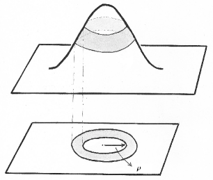
Figure 1: A stretched strip on a bump and its downward projection on a flat plane.

The Gaussian bump (14) also introduces a characteristic length on the surface. By vertically stretching the surface, the amount of area in the stretched strip is increased with respect to its projection on the plane which is depicted in Figure (1). As a result, the quantum particle would rather remain localized when it is situated near the maximal stretch of the surface thus introducing a scale of the order of the dispersion $\sigma_{0}$ of the profile (14). This can easily be seen when looking at the Heisenberg uncertainty relation $\delta p\delta x\sim\hbar$: $\delta x$ is bigger in the stretched area. Hence, it is energetically favorable the quantum particle migrates to the stretched area of the bump thus creating charge distribution if it itself is charged. This charge density is exactly depicted by the probability density of finding the particle in a specific place on the surface.

Since we are interested in bound states now we consider only particles with $\boldsymbol{\rm m}=0$, since only for them the potential $W_{\boldsymbol{\rm 0}}$ is negative and they will bind with different quantized energies. Equating the kinetic and potential energy terms we provide a rough estimate of the order of magnitude of the bound state energies, namely $E<-\hbar^{2}/2m\sigma_{0}^{2}$. Later on in the text we will see that this estimate is correct up to a geometry dependent factor $A_{0}^{2}/\sigma_{0}^{2}$, which measures the flatness of the profile.

Obtaining a solution to equation (11) is not an easier task than solving the original one. Nevertheless, we can be sure that bound states do exist since we have transformed the problem to a one-dimensional one with a negative potentialLL . Using an approximation we can transform this equation into simpler one thus providing us with a chance to generate an approximate wave function. The behaviour of the wave function in the vicinity of the origin, that is $\rho\to 0$ can be considered as a starting point in our consideration. In that particular limit $x\approx\rho$ due to (9) and $\lim_{\rho\to 0}\dot{f}=0$ (for the Gaussian bump) for the potential $W_{\boldsymbol{\rm 0}}(x)$ we have

$$W_{\boldsymbol{\rm 0}}\left[x\right]=-\frac{1}{4x^{2}}-\frac{A_{0}^{2}}{\sigma_{0}^{2}}\frac{1}{\sigma_{0}^{2}}.$$ (15)

Equation (11) with the above potential possesses a stable negative energy solution with $k^{\prime 2}={2m|E|}/{\hbar^{2}}-{A_{0}^{2}}/{\sigma_{0}^{4}}$ provided ${2m|E|}/{\hbar^{2}}>{A_{0}^{2}}/{\sigma_{0}^{4}}$. Here ${A_{0}^{2}}/{\sigma_{0}^{2}}$ is a measure of the flatness of the Gaussian bump. Due to the sign change of the energy the ordinary Bessel functions $J_{\boldsymbol{\rm 0}}$ and $Y_{\boldsymbol{\rm 0}}$ which solve equation (11) with the above potential (15) turn into the modified Bessel functions $I_{\boldsymbol{\rm 0}}$ and $K_{\boldsymbol{\rm 0}}$Abr&Steg . Since the modified Bessel function $I_{\boldsymbol{\rm 0}}$ increases exponentially for large distances, whereas $K_{\boldsymbol{\rm 0}}$ decreases, the boundary conditions imposed by the asymptotic flatness of the Gaussian bump and the need for a squared integrable wave function, we select $K_{\boldsymbol{\rm 0}}$. Thus the solution in the vicinity of $x\to 0$ is expressed with the modified Bessel function

$$F_{{\boldsymbol{\rm 0}}}(x)\approx\sqrt{x}K_{\boldsymbol{\rm 0}}(k^{\prime}x).$$

Having deduced the correct behaviour of the wave function in the vicinity of the origin we can try to solve equation (11) with the ansatz

$$F_{\boldsymbol{\rm 0}}(x)=\exp\left[\frac{i}{\hbar}S(x)\right]\sqrt{x}K_{\boldsymbol{\rm 0}}(k^{\prime}x).$$ (16)

Using the fact that $K_{\boldsymbol{\rm 0}}$ satisfies the Bessel equation we end up with an approximate equation for $S(x)$

$$\frac{i}{\hbar}S^{{}^{\prime\prime}}=\frac{1}{\hbar^{2}}\left(S^{{}^{\prime}}\right)^{2}+\frac{i}{\hbar}\frac{S^{{}^{\prime}}}{x}-\left[\frac{1}{4}\frac{\ddot{f}^{2}}{\left(1+\dot{f}^{2}\right)^{3}}-\frac{A_{0}^{2}}{\sigma_{0}^{4}}\right],$$ (17)

where hereafter $(\;^{{}^{\prime}})$ denotes differentiation with respect to $x$. In the derivation of (17) we kept in mind that $x\approx\rho$ and approximated $1/\rho^{2}$ with $1/x^{2}$ in the potential (12). We have also approximated ${dK_{\boldsymbol{\rm 0}}}/{dx}\approx-K_{\boldsymbol{\rm 0}}/x$ which preserved the behaviour near the origin.

Next we expand $S(x)$ in series with increasing powers of the small parameter $\hbar$ à la WKB type expansion

$$S(x)=S_{0}(x)+i\hbar S_{1}(x)+\ldots$$

and obtain for the first two functions in the expansion the equations

$$S_{0}^{{}^{\prime}} = 0\quad\Rightarrow\quad S_{0}={\rm const},$$ (18)

$$S_{0}^{{}^{\prime\prime}} = 2S_{0}^{{}^{\prime}}S_{1}^{{}^{\prime}}+S_{0}^{{}^{\prime}}/x\quad\Rightarrow\quad\forall S_{1}^{{}^{\prime}},$$

$$S_{1}^{{}^{\prime\prime}} = (S_{1}^{{}^{\prime}})^{2}+S_{1}^{{}^{\prime}}/x-\left(\frac{A_{0}^{2}}{\sigma_{0}^{4}}-\frac{1}{4}\frac{\ddot{f}^{2}}{\left(1+\dot{f}^{2}\right)^{3}}\right).$$ (19)

Solving (19) we assume that i.) $(S_{1}^{{}^{\prime}})^{2}\gg S_{1}^{{}^{\prime\prime}}$ and ii.) $(S_{1}^{{}^{\prime}})^{2}\gg S_{1}^{{}^{\prime}}/x$ to obtain

$$S_{1}^{{}^{\prime}}=\pm\sqrt{\frac{A_{0}^{2}}{\sigma_{0}^{4}}-\frac{1}{4}\frac{\ddot{f}^{2}}{\left(1+\dot{f}^{2}\right)^{3}}}.$$ (20)

From the form of the solution we see that the assumptions i.) and ii.) we made in deriving it are justified away from the origin. Since we already dealt with the behaviour of the wave function in the vicinity of that point we write

$$F_{\boldsymbol{\rm 0}}(x)=\frac{e^{iS_{0}/\hbar}}{\sqrt{2\pi N^{2}}}\sqrt{x}K_{\boldsymbol{\rm 0}}(k^{\prime}x)\exp\left[-\int_{0}^{x}S_{1}^{{}^{\prime}}dx\right],$$ (21)

where we have chosen the $+$ sign solution of (20), ameliorating the vanishing behaviour of the wave function at infinity. The norm $N^{2}$ is calculated using (13). The logarithmic divergence at the origin of the modified Bessel function of second kind $K_{\boldsymbol{\rm 0}}$ is regularized by the extra factor proportional to $\sqrt{x}$ in terms of the Euclidean line length on the surface, making the probability density to find the particle at the origin vanishing. Moreover, since (21) vanishes exponentially for large distances, the radial probability displays a maximum close to the origin, which is exactly the behaviour of the expectation value that we already deduced from the considerations using Heisenberg’s principle.

As a result, particles with $\boldsymbol{\rm m}=0$ concentrate in a ring shaped region on the surface of the Gaussian bump around the axis of symmetry.

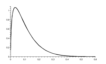
Figure 2: The probability density $|\psi_{\boldsymbol{\rm 0}}(\rho)|^{2}\sqrt{g}$ (vertical axis) to find a particle between $\rho$ and $\rho+d\rho$ (horizontal axis) for the Gaussian bump. Here we have set $A_{0}=\sigma_{0}=1$ and $k^{\prime}=5$. The initial phase $S_{0}=0$.

Figure (2) depicts thus generated probability density $|\psi_{\boldsymbol{\rm 0}}(\rho)|^{2}\sqrt{g}$ of finding the particle in a state with angular momentum $\boldsymbol{\rm m}=0$ between $\rho$ and $\rho+d\rho$ in terms of the distance from the axis of symmetry and clearly shows that the probability of finding the quantum particle is biggest at the stretched area of the bump as already discussed. This shows that the approximations which lead to (21) are fully justified. They also show the way to a proper test function for a run of the variational method to determine the ground state energy and wave function, which must not have nodes – a property clearly visible in (21). This is a matter of a future study.

Here we do not present an estimate of the structure of the energy spectrum except the already stated fact – the discrete spectrum starts at $E<-\hbar^{2}A_{0}^{2}/2m\sigma_{0}^{4}$, value which is determined by the geometrical extensions of the Gaussian bump. Over that value the motion of a particle with $\boldsymbol{\rm m}=0$ is classically infinite and hence the wave function is supposed to be in the form of a plane wave. What is, at least, the approximate expression of that plane wave?

We propose to look for solutions of (11) in the form of

$$F_{\boldsymbol{\rm 0}}^{\rm cont}=f_{\boldsymbol{\rm 0}}(x)\exp{\left(\pm i\int Q_{\boldsymbol{\rm 0}}dx\right)},$$ (22)

where $Q_{\boldsymbol{\rm 0}}\approx\sqrt{k_{1}^{2}/4+1/4x^{2}+k^{2}}$. Here $f_{\boldsymbol{\rm 0}}(x)$ is fast changing function, such that $F_{\boldsymbol{\rm 0}}^{{}^{\prime\prime}}(x)\approx\left(-Q_{\boldsymbol{\rm 0}}^{2}\pm 2iQ_{\boldsymbol{\rm 0}}f_{\boldsymbol{\rm 0}}^{{}^{\prime}}/f_{\boldsymbol{\rm 0}}\pm iQ_{\boldsymbol{\rm 0}}^{{}^{\prime}}\right)F_{\boldsymbol{\rm 0}}$. From here and (11) we see that

$$\frac{f_{\boldsymbol{\rm 0}}^{{}^{\prime}}}{f_{\boldsymbol{\rm 0}}}\approx-\frac{1}{2}\frac{Q_{\boldsymbol{\rm 0}}^{{}^{\prime}}}{Q_{\boldsymbol{\rm 0}}}\quad\Rightarrow\quad f_{\boldsymbol{\rm 0}}\sim 1/\sqrt{Q_{\boldsymbol{\rm 0}}}.$$ (23)

Hence we write

$$F_{\boldsymbol{\rm 0}}^{\rm cont}(x)=\frac{\exp{\left(\pm i\int\sqrt{k_{1}^{2}/4+1/4x^{2}+k^{2}}dx\right)}}{\left(k_{1}^{2}/4+1/4x^{2}+k^{2}\right)^{1/4}},$$ (24)

where the plane wave exhibits a node in the origin.

The energy spectrum for particles with non-vanishing angular momentum is continuous and starts at $E=0$. Good approximate solutions of (11) are the ordinary Bessel functions $\sqrt{x}J_{\boldsymbol{\rm m}}(kx)$ and $\sqrt{x}Y_{\boldsymbol{\rm m}}(kx)$, whose argument is the Euclidean line length on the surface.

Let us now turn our attention to the inverse problem or equivalently the question ”What rotationally invariant surface leads to an effective geometry induced potential $W_{\boldsymbol{\rm m}}$ that equals prescribed negative function $-U[x(\rho)]$, where $U\geq 0$ for $\forall\rho$?” (negative because we are primary interested in bound states). This question is of particular interest since for certain classes of negative potentials $-U$ we already know the exact wave functions which can readily be used in revealing the particle’s distribution on the surface. The solution of the inverse problem goes through the recognition of its equivalence with the following differential equation (see equations (12) and (5)):

$$\frac{1}{4}\frac{\ddot{f}(\rho)^{2}}{\left(1+\dot{f}(\rho)^{2}\right)^{3}}=U(\rho)+\frac{\boldsymbol{\rm m}^{2}-1/4}{\rho^{2}}.$$ (25)

From equations (5) and (25) one can easily deduce a condition on $k_{1}(\rho)$ in order to have a binding potential for a particle with $\boldsymbol{\rm m}\neq 0$, i.e.

$$k_{1}^{2}>\frac{4\boldsymbol{\rm m}^{2}-1}{\rho^{2}}.$$

For smooth surfaces at $\rho=0$ this means that there will be only strips where this condition holds. For flat surfaces where $k_{1}=0$ this condition implies that only particles with $\boldsymbol{\rm m}=0$ bind, a fact previously noticed incirone*01 ; berry*73 . Now we try to solve equation (25) using substitution $\dot{f}=\sinh{(\omega)}$ (here $\omega=\omega(\rho)$) to end up with the linear equation

$$\frac{1}{2}\frac{d\tanh(\omega)}{d\rho}=\pm\sqrt{U(\rho)+\frac{\boldsymbol{\rm m}^{2}-1/4}{\rho^{2}}},$$ (26)

which can be solved thus yielding a result for $\dot{f}(\rho)$. We integrate to obtain the profile of the surface

$$f(\rho)=\pm\int^{\rho}_{\rho_{1}}\frac{|\mathcal{A}|}{\sqrt{1-\mathcal{A}^{2}}}d\rho^{\prime},$$ (27)

where

$$\mathcal{A}(\rho)=\pm 2\int^{\rho}_{\rho_{0}}\sqrt{U(\rho^{\prime})+\frac{\boldsymbol{\rm m}^{2}-1/4}{{\rho^{\prime}}^{2}}}d\rho^{\prime}.$$ (28)

Here $\rho_{0}$ and $\rho_{1}$ are constants of integration and are to be determined by the boundary conditions due to the behavior of the function $U$ representing the potential we want to model. Since ${f}(\rho)$ takes only real values (the same is true for all of its derivatives, i.e. ${d^{\rm n}f}/{d\rho^{\rm n}}\in\mathbb{R}$ for ${\rm n}=0,1,\ldots$) as a function describing the profile of a surface we impose $0<|\mathcal{A}|<1$. The $\mathcal{A}=0$ case is realized by a flat surface. Using the theorem of the mean value in (28) and the above inequality we obtain

$$\rho_{0}<\rho<\rho_{0}+\frac{1}{2}\left|U(\xi)+\frac{\boldsymbol{\rm m}^{2}-1/4}{{\xi}^{2}}\right|^{-1/2},$$ (29)

where the point $\xi\in[\rho_{0},\rho]$. In that manner we show that for generic angular momentum $\boldsymbol{\rm m}$ and non-zero potential $U$ the corresponding rotational surface creating this potential and allowing a bound state of a quantum particle with ${\boldsymbol{\rm m}}\neq 0$ exists only in a ribbon, a circular strip around the axis of symmetry.

Let us also note that for $\boldsymbol{\rm m}\neq 0$ the bump (a macroscopic structure) has a magnetic moment, i.e. the macroscopic deformation of the surface acquires quantum number. Indeed the probability density current $\vec{J}$ (${\rm div}\vec{J}=0$) associated with the wave function $\chi_{\rm t}$ is given by

$$\vec{J}=\left(J_{\phi},J_{\rho},J_{z}\right)=\frac{\hbar}{m}\left(\boldsymbol{\rm m}\frac{|\psi_{\boldsymbol{\rm m}}|^{2}}{\rho},{\rm Re}\frac{\psi_{\boldsymbol{\rm m}}^{\ast}\partial_{\rho}\psi_{\boldsymbol{\rm m}}}{i\sqrt{1+\dot{f}^{2}}},0\right),$$

where $J_{\phi},J_{\rho}$ and $J_{z}$ are the components of the vector $\vec{J}$ in the orthonormal right-handed triad $(\vec{e}_{\rho},\vec{e}_{\phi},\vec{e}_{z})$, has nonzero and quantized with $\boldsymbol{\rm m}$ circulation along the circumference of the bump.

Now let us give a couple of examples:

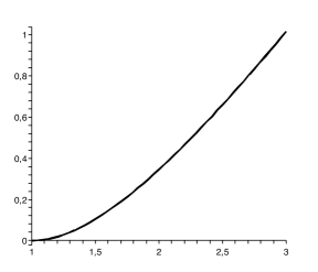
Figure 3: The surface $f(\rho)/\rho_{0}$ (vertical axis) with a cusp on which a particle with $\boldsymbol{\rm m}=0$ moves freely. On the horizontal axis is plotted $\rho/\rho_{0}$. At infinity that surface tends to a cone.

• $U=0$, i.e. free motion; From (28) and (27) it follows that

  $$f^{\rm free}_{\boldsymbol{\rm m}}(\rho)=\pm\rho_{0}\int^{\rho/\rho_{0}}_{\rho_{1}/\rho_{0}}\frac{\sqrt{|4\boldsymbol{\rm m}^{2}-1|}\left|\ln\left(\rho^{\prime}\right)\right|}{\sqrt{1-(4\boldsymbol{\rm m}^{2}-1)\;\ln^{2}\left(\rho^{\prime}\right)}}d\rho^{\prime}.$$ (30)

  Here $\rho_{0}$ determines the characteristic scale of the surface on which we consider this free quantum problem. Its magnitude can be chosen in $[\mu m]$ or $[nm]$ depending on the scale that we want to model. If we consider the shape of a surface allowing a free motion of a particle with zero angular momentum, that is $\boldsymbol{\rm m}=0$, we can integrate (30) with $\rho_{1}=\rho_{0}$ to produce Figure (3). That surface is asymptotically flat as it tends to a cone $f^{{\rm free}}_{\boldsymbol{\rm 0}}(\rho)\to\rho$ as $\rho\to\infty$.

  Next we consider the strip of a surface allowing a free motion of a particle with non-zero angular momentum, that is $\boldsymbol{\rm m}\neq 0$. We can impose the condition $1>(4\boldsymbol{\rm m}^{2}-1)\;\ln^{2}\left(\rho/\rho_{0}\right)$ to find the extensions of the strip

  $$\rho_{0}<\rho<\rho_{0}\exp{\left[(4\boldsymbol{\rm m}^{2}-1)^{-1/2}\right]}.$$ (31)

  Since the problem is defined on a strip, we can quantize it in the usual finite volume method, which would lead to standing wave solutions on the surface. Their energy is

  $$E_{n}^{\boldsymbol{\rm m}}(\rho_{0})=\frac{2\pi^{2}\hbar^{2}n^{2}}{m\rho_{0}^{2}\left[e^{(4\boldsymbol{\rm m}^{2}-1)^{-1/2}}-1\right]^{2}}.$$ (32)

• $U=\omega^{2}\rho^{2}$, i.e. harmonic oscillator potential; From (28) it follows that

  $$\mathcal{A}^{{\rm harm}}_{\boldsymbol{\rm m}}(\rho)=\pm 2\int^{\rho}_{\rho_{0}}\sqrt{\omega^{2}{\rho^{\prime}}^{2}+\frac{\boldsymbol{\rm m}^{2}-1/4}{{\rho^{\prime}}^{2}}}d\rho^{\prime}.$$ (33)

  Let us consider two cases consequently:

  I.) The ${\boldsymbol{\rm m}}=0$ case yields for (33) the result

  $$\mathcal{A}^{{\rm harm}}_{\boldsymbol{\rm 0}}(\rho) = \pm\frac{1}{2}\left\{\sqrt{4\omega^{2}\rho^{4}-1}\right.$$ (34)

  $$+\left.\arctan{\left[\left(4\omega^{2}\rho^{4}-1\right)^{-1/2}\right]}-\frac{\pi}{2}\right\},$$

  where we have set the value of $\rho_{0}=1/\sqrt{2|\omega|}$. From the requirement $0<|\mathcal{A}^{{\rm harm}}_{\boldsymbol{\rm 0}}|<1$ we obtain the following estimate

  $$\rho<\frac{\left(1+(2+\varepsilon)^{2}\right)^{1/4}}{\sqrt{2|\omega|}}\approx\frac{5^{1/4}+{\varepsilon}/{5^{3/4}}}{\sqrt{2|\omega|}},$$ (35)

  where $\varepsilon={\pi}/{2}-\arctan{\left(4\omega^{2}\rho^{4}-1\right)^{-1/2}}\ll 1$. Thus we find an expression for the extensions of the circular strip of a rotational surface creating harmonic potential and allowing a bound state of a particle with vanishing angular momentum in a harmonic oscillator potential

  $$\frac{1}{\sqrt{2|\omega|}}\leq\rho<\left(5^{1/4}+\frac{\varepsilon}{5^{3/4}}\right)\frac{1}{\sqrt{2|\omega|}}.$$ (36)

  II.) The ${\boldsymbol{\rm m}}\neq 0$ case yields for (33) the result

  $$\pm\mathcal{A}^{{\rm harm}}_{\boldsymbol{\rm m}}(\rho)=\sqrt{\omega^{2}{\rho}^{4}+{\boldsymbol{\rm m}^{2}-1/4}}-\sqrt{\boldsymbol{\rm m}^{2}-1/4}\;{\rm arctanh}{\left[\left(1+\frac{\omega^{2}\rho^{4}}{\boldsymbol{\rm m}^{2}-1/4}\right)^{-1/2}\right]}.$$ (37)

  Next we impose the condition $0<|\mathcal{A}^{{\rm harm}}_{\boldsymbol{\rm m}}|<1$ and numerically find for $\boldsymbol{\rm m}=1,2,3$ particles

  $$1.071<\sqrt{2\omega}\rho<1.602\qquad\boldsymbol{\rm m}=1,$$

  $$1.602<\sqrt{2\omega}\rho<1.957\qquad\boldsymbol{\rm m}=2,$$ (38)

  $$1.980<\sqrt{2\omega}\rho<2.265\qquad\boldsymbol{\rm m}=3.$$

In conclusion we have calculated the quantum potential associated with a Gaussian deformation of a two-dimensional plane. For that simple surface deformation we have shown that a quantum binding force of geometric origin attracts only particles with $\boldsymbol{\rm m}=0$ to the origin. Further, we have solved the inverse problem and have shown that surfaces in a form of a ribbon allow bound states of particles with generic angular momenta. Thus we speculate that a classical object (the ribbon) exhibits quantum characteristics (the magnetic moment due to non-vanishing quantized probability current circulation along the circumference) acquired due to curvature. We have also found and depicted the surface which corresponds to a free motion of a particle with vanishing angular momentum.

References

- (1) R. Kamien, Science 299, 1671, (2003).
- (2) D. Caspar and A. Klug, Principles in the Construction of Regular Viruses (NY, Cold Spring Harbor: Cold Spring Harbor Laboratory) Cold Spring Harbor Symposium on Quantitative Biology vol. 27 p. 1, (1962).
- (3) V. Vitelli and A. Turner, Phys. Rev. Lett. 93, 215301, (2004).
- (4) M. Entin and L. Magarill, Phys. Rev. B 64, 085330, (2001).
- (5) J. Goldstone and R. Jaffe, Phys. Rev. B 45, 14100, (1992).
- (6) P. Exner and P. Seba, Journ. Math. Phys. 30, 2574, (1989). 2893
- (7) M. Encinosa and B. Etemadi, Phys. Rev. A 58, 77, (1998).
- (8) M. Encinosa and L. Mott, Phys. Rev. A 68, 014102, (2003).
- (9) L. Kaplan, N. Maitra and E. Heller, Phys. Rev. A 56, 2592, (1997).
- (10) K. Mitchell, Phys. Rev. A 63, 042112, (2001).
- (11) R. Schult, D. Ravenhall and H. Wyld, Phys. Rev. B 39, 5476, (1989).
- (12) J. Carini, J. Londergan, D. Murdock and C. Yung, Phys. Rev. B 55, 9842, (1997).
- (13) R. Dandoloff and R. Balakrishnan, Journ. Phys. A 38, 6121, (2005).
- (14) R. Dandoloff and T.T. Truong, Phys.Lett. A, 325, 233, (2004).
- (15) H. Jensen and H. Koppe, Ann. Phys. (N.Y.), 63, 586, (1971).
- (16) R. C. T. da Costa Phys. Rev. A 23, 1982, (1981).
- (17) P. Duclos, P. Exner and D. Krejcirik, Commun. Math. Phys. 223, 13, (2001).
- (18) R. Courant and D. Hilbert, Methods of Mathematical Physics, Wiley-Interscience, New York, (1953), vol.1
- (19) L.D. Landau and E.M. Lifshitz, Quantum Mechanics, Pergamon Press, Oxford, (1987).
- (20) M. Abramowitz and I. Stegun, Handbook of Mathematical Functions, Dover Publications, New York, (1965).
- (21) M. Cirone, K. Rzazewski , W Schleich , F Straub and J. A. Wheeler, Phys. Rev. A 65, 022101, (2001).
- (22) M. Berry and A. Ozorio de Almeida, Journ. Phys. A 6, 1451, (1973).