Also at] Laboratoire de Physique Théorique et Modélisation , Université de Cergy-Pontoise, F-95302 Cergy-Pontoise, France

Curvature-induced quantum behaviour on a helical nanotube

Abstract

We investigate the effect of curvature on the behaviour of a quantum particle bound to move on a surface shaped as a helical tube. We derive and discuss the governing Schrödinger equation and the corresponding quantum effective potential which is periodic and points to the helical configuration as more energetically favorable as compared to the straight tube. The exhibited periodicity also leads to energy band structure of pure geometrical origin.

Recent developments in nanotechnologyAFS made it possible to grow quasi-two-dimensional surfaces of arbitrary shape where quantum and curvature effects play a major roleMT . Examples include single crystal $\rm NbSe_{3}$ Möbius stripsTTOIYH , spherical $\rm CdSe-ZnS$ core-shell quantum dotsSWFEB , $\rm Si$ nanowire, nanoribbon transistorsDNSPEG , quantum waveguidesLCM and nanotorustorus . Several publicationsINTT ; Clark*96 ; Exner*95 ; Exner*01 ; Fujita*04 ; Kaplan ; Mitchell have treated the constrainment of quantum-mechanical particles (with applications in, e.g. standard Schödinger equation problemsJaffe*03 and relativistic Dirac equation problemsJaffe*99 ; BJ*93 ) to a two-dimensional surface since the original works by Jensen and Koppe, da CostaJK*71 ; daCosta*81 ; daCosta*82 . Since two-dimensional systems are an a priori idealization it is reasonable to quantize before constraining the particle to the nanotube. As a result a quantum particle confined to a two-dimensional surface embedded in $\mathbb{R}^{3}$ experiences a potential that is a function of the Mean and the Gauss curvatures of the surfacedaCosta*81 ; daCosta*82 . This curvature-induced quantum potential is a geometrical invariant which property lead the authorsvic*07 to pose the inverse differential geometrical problem: what curved surfaces produce prescribed curvature-induced potential.

Possible physical applications of the above include the geometric interaction between defects and curvature in thin layers of superfluids, superconductors, and liquid crystals deposited on curved surfacesVit*04 ; the curvature of a semiconductor surface determines also an interesting mechanism of spin–orbit interaction of electronsEnt*01 ; a charged quantum particle trapped in a potential of quantum nature due to bending of an elastically deformable thin tube travels without dissipation like a solitonDan*05 ; the twist of a strip plays a role of a magnetic field and is responsible for the appearance of localized states and an effective transverse electric field thus reminisce the quantum Hall effectDan*04 .

Now let us turn our attention to the geometrical realization of the helical tube.

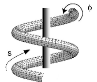
Figure 1: The geometry of an infinite helical tube may be parametrized by two families of space curves (see equation (5) and text).

One can associate with a space curve $\vec{\bf x}(s)$ at any point $s$ along it a moving frame consisting of three vectors $\vec{\bf t}$–tangent, $\vec{\bf n}$–normal and $\vec{\bf b}$–binormal and evolving along the curve according to the Frenet-Serret equations:

$$\dot{\vec{{\bf t}}}=\vec{\omega}\wedge\vec{{\bf t}},\qquad\dot{\vec{{\bf b}}}=\vec{\omega}\wedge\vec{{\bf b}},\qquad\dot{\vec{{\bf n}}}=\vec{\omega}\wedge\vec{{\bf n}},$$ (1)

where $\vec{\omega}$ is the instantaneous angular velocity of the Frenet-Serret frame where the arclength $s$ plays the role of time. Hereafter the dot denotes derivation with respect to the natural parameter $s.$ Here $\kappa(s)$ and $\tau(s)$ are the curvature and torsion of the space curve.

Since $\vec{\omega}$ has a component along $\vec{{\bf t}}$ we redefine the frame vectors

$$\vec{{\bf N}}=\cos{\theta(s)}\vec{{\bf n}}+\sin{\theta(s)}\vec{{\bf b}}, \dot{\vec{{\bf N}}}=\vec{\Omega}\wedge\vec{{\bf N}}$$ (2)

$$\vec{{\bf B}}=-\sin{\theta(s)}\vec{{\bf n}}+\cos{\theta(s)}\vec{{\bf b}}, \dot{\vec{{\bf B}}}=\vec{\Omega}\wedge\vec{{\bf B}}.$$ (3)

We choose $\theta(s)$ so that $\vec{\Omega}$ has no component in the direction of $\vec{{\bf t}}$. A brief calculation yields

$$\theta(s)=-\int_{s_{0}}^{s}ds^{{}^{\prime}}\tau(s^{{}^{\prime}}).$$ (4)

Figure 2: The cross-section of the nanotube in Fig. 1.

Now let us mount a disc $D$ rigidly in the reference frame where $\vec{{\bf N}}$ and $\vec{{\bf B}}$ are at rest, i.e. the Fermi-Walker frameGold&Jaffe*92 . The points on the surface may be parametrized by

$$\vec{{\bf X}}(s,\phi)=\vec{\bf x}(s)-\rho_{0}\left\{\sin{\phi}\vec{{\bf B}}+\cos{\phi}\vec{{\bf N}}\right\}.$$ (5)

The two families of space curves weaving the above surface in $\mathbb{R}^{3}$ are the following. The first is a circle parametrized by the angle $\phi$ and is actually the rim of the disc that is rigidly mounted to the tangent of $\vec{\bf x}(s)$ at each point in space. The tip of the vector in the disc from the central axis to the rim is denoted by $\rho_{0}\cos{\phi}\vec{{\bf N}}+\rho_{0}\sin{\phi}\vec{{\bf B}}.$ Its origin coincides with the helical space line $\vec{\bf x}(s).$ The second is given by the lines with tangent passing through each point of the first family. Refer to Figure 1 for the visual expression of the above construction.

In this article we will study the properties of the Schrödinger equation on that surface.

The line element is

$$|d\vec{{\bf X}}|^{2}=d\varphi^{2}+h^{2}ds^{2},$$ (6)

where

$$h(s,\phi)=1+\rho_{0}\kappa(s)\cos{\left[\theta(s)+\frac{\varphi}{\rho_{0}}\right]}$$ (7)

and

$$\varphi=\rho_{0}\phi$$ (8)

has a dimension of length.

If we change the parametrization $s\rightarrow-s$ and $\varphi\rightarrow-\varphi$ this would mean that we evolve the surface backward from a certain arbitrary point $s_{0}$ of the infinite space line $\vec{\bf x}(s).$ The torsion $\tau$ exhibits invariance $\tau(s)=\tau(-s)$ and the surface element must remain unchanged.

$$\theta(-s)+\left(-\frac{\varphi}{\rho_{0}}\right)\rightarrow-\left[\theta(s)+\frac{\varphi}{\rho_{0}}\right],\quad h(s)\rightarrow h(-s).$$

Thus we show that the line element is indeed invariant

$$|d\vec{{\bf X}}(s,\varphi)|^{2}=|d\vec{{\bf X}}(-s,-\varphi)|^{2}.$$

From formulas (2) and (3) we see that at $\theta(s)=0$, that is at $s=0$ if $s_{0}=0$ (see (4)), we have the coincidence $\vec{{\bf N}}\equiv\vec{{\bf n}}$ and $\vec{{\bf B}}\equiv\vec{{\bf b}}.$ The normal $\vec{{\bf n}}$ always points towards the axis around which the helix is wound, i.e. it points inward. From (7) it is clear that $h(0,0)=1+\rho_{0}\kappa(0)>1-\rho_{0}\kappa(0)=h(0,\pi).$ The surface is stretched more on the outside thus we have a natural choice of the origin (the outer intersection of the ray through $\vec{{\bf n}}$ and the cross-section of the tube) for the two families of curves (see Figure 2).

Introducing the normal to the surface $\vec{\nu}$ from the Gauss triad $\vec{\nu}=\partial_{\varphi}\vec{{\bf X}}\wedge\partial_{s}\vec{{\bf X}}\left|\partial_{\varphi}\vec{{\bf X}}\wedge\partial_{s}\vec{{\bf X}}\right|^{-1/2}$ we can compute the linear Weingarten map $\left(\begin{array}[]{c}\partial_{\varphi}\vec{\nu}\\ \partial_{s}\vec{\nu}\\ \end{array}\right)=W\left(\begin{array}[]{c}\partial_{\varphi}\vec{{\bf X}}\\ \partial_{s}\vec{{\bf X}}\\ \end{array}\right),$ where $W$ is the matrix realizing the map of the tangent space in itself

$$W=\left(\begin{array}[]{cc}\rho_{0}^{-1}&0\\ 0&\kappa(s)\cos\left[\theta(s)+\frac{\varphi}{\rho_{0}}\right]h^{-1}\\ \end{array}\right).$$ (9)

With the help of (9) we may compute

$$M=\frac{1}{2}(\kappa_{1}+\kappa_{2})=-\frac{1}{2}{\rm tr}(W),\quad K=\kappa_{1}\kappa_{2}=\det(W),$$

the Mean and the Gauss curvatures of the surface respectively, where $\kappa_{1}$ and $\kappa_{2}$ are the principal curvatures of the surface. They are also the eigenvalues of the Weingarten matrix (9). Thus we obtain

$$\kappa_{1}=\frac{1}{\rho_{0}},\qquad\kappa_{2}=\kappa(s)\cos\left[\theta(s)+\frac{\varphi}{\rho_{0}}\right]h^{-1}.$$ (10)

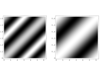
Figure 3: Density plot of the potentials $V_{\rm eff}(s,\varphi)$ on the left and $V_{\rm curv}(s,\varphi)$ on the right. Along the horizontal axis is the natural parameter $s$, where $s\in[0,2\pi]$; $\phi$ is on the vertical axis $\varphi\in[0,\rho_{0}2\pi]$. Here $\tau=\kappa=1$ and $\rho_{0}=10^{-1}$. Lighter regions correspond to higher values of the potential and lower probability to find a particle there, respectively.

Since we study the resulting Schrödinger equation for a particle confined to move on that surface and following da Costa an effective potential appears in the Schrödinger equation which has the following form:

$$V_{\rm curv} = -\frac{\hbar^{2}}{2\mu}(M^{2}-K)$$

$$= -\frac{\hbar^{2}}{2\mu}\left[\frac{1}{4}({\rm tr}W)^{2}-\det(W)\right]$$

where $\mu$ is the effective particle’s mass, $\hbar$–Plank’s constant; $V_{\rm curv}$ depends on $s$ and $\varphi$ which appear as the generalized coordinates on the surface; $M=(\kappa_{1}+\kappa_{2})/2$ and $K=\kappa_{1}\kappa_{2}$ are the Mean and the Gauss curvatures respectively. For the surface (5) we obtain

$$V_{\rm curv}(s,\varphi)=-\frac{\hbar^{2}}{8\mu}\frac{1}{\rho_{0}^{2}}\frac{1}{h^{2}}.$$ (12)

From equations (6) and (7) it follows that the surface is more stretched on the outside, that is at $\varphi=0$ (see Figure 2), because $h(0,0)>h(0,\pi).$ The Heisenberg uncertainty principle states that a particle would have a lower energy where the line element is bigger. Our expectation is that the probability to find a particle on the outer rim of the surface is maximal. This guiding principle will allow us to interpret the appropriate effective Schrödinger equation whose potential possesses the above property.

The Laplace-Beltrami operator (the quantum mechanical kinetic term) in the coordinate system (5) can be written as follows:

$$-\triangle_{s,\varphi}\Psi = -\frac{1}{h^{2}}\frac{\partial^{2}\Psi}{\partial s^{2}}-\frac{\partial^{2}\Psi}{\partial\varphi^{2}}+\kappa\sin{\left(\theta+\frac{\varphi}{\rho_{0}}\right)}\frac{1}{h}\frac{\partial\Psi}{\partial\varphi}$$

$$+ \rho_{0}\dot{\kappa}(s)\cos{\left(\theta(s)+\frac{\varphi}{\rho_{0}}\right)}\frac{1}{h^{3}}\frac{\partial\Psi}{\partial s}$$

$$- \rho_{0}\dot{\theta}(s)\kappa(s)\sin{\left(\theta(s)+\frac{\varphi}{\rho_{0}}\right)}\frac{1}{h^{3}}\frac{\partial\Psi}{\partial s}.$$

Here $\Psi$ as a solution must be normalized as $\int|\Psi|^{2}dS=1.$ We introduce $\Phi=\sqrt{h}\Psi$ and the wave function will be normalized with respect to the usual flat norm on a rectangular domain determined by the periodic properties of $h[\theta(s),\varphi],$ that is $\int_{-\rho_{0}\pi}^{\rho_{0}\pi}d\varphi\int_{s_{a}}^{s_{b}}ds|\Phi|^{2}=1,$ where $s_{a}$ and $s_{b}$ are such that $\theta(s_{a})=-\theta(s_{b})=\pi.$ Then:

$$-\sqrt{h}\triangle\frac{\Phi}{\sqrt{h}} = -\frac{1}{h^{2}}\frac{\partial^{2}\Phi}{\partial s^{2}}-\frac{\partial^{2}\Phi}{\partial\varphi^{2}}+2\frac{\partial_{s}h}{h^{3}}\frac{\partial\Phi}{\partial s}+V_{\rm kin}\Phi,\qquad$$ (14)

where

$$V_{\rm kin}=\frac{1}{2}\frac{\partial_{\varphi}^{2}h}{h}-\frac{1}{4}\frac{(\partial_{\varphi}h)^{2}}{h^{2}}+\frac{1}{2}\frac{\partial_{s}^{2}h}{h^{3}}-\frac{5}{4}\frac{(\partial_{s}h)^{2}}{h^{4}}.$$ (15)

Now we obtain a differential equation which for the helical tube is to be written with $\kappa$ and $\tau$ constants:

$$-\frac{1}{h^{2}}\frac{\partial^{2}\Phi}{\partial s^{2}}-\frac{\partial^{2}\Phi}{\partial\varphi^{2}}+2\frac{\partial_{s}h}{h^{3}}\frac{\partial\Phi}{\partial s}+V_{\rm eff}\Phi-k^{2}\Phi=0,$$ (16)

where

$$V_{\rm eff}(s,\varphi) = V_{\rm kin}+\frac{2\mu}{\hbar^{2}}V_{\rm curv}$$

$$= \frac{\partial_{\varphi}^{2}h}{2h}-\frac{(\partial_{\varphi}h)^{2}}{4h^{2}}+\frac{\partial_{s}^{2}h}{2h^{3}}-\frac{5}{4}\frac{(\partial_{s}h)^{2}}{h^{4}}-\frac{1}{4}\frac{1}{\rho_{0}^{2}h^{2}}.$$

Here $k$ is the wave number ($k^{2}=2\mu E/\hbar^{2}$). The corresponding spatial configuration for which equation (16) serves as an effective Schrödinger equation is depicted in Figure 1.

Fixing $s=0$ a straight-farward check provides us with the estimate

$$V_{\rm eff}(\varphi=0)<V_{\rm eff}(\varphi=\pi)$$

and since the probability amplitude follows the behaviour of potential the probability to find the particle on the outer rim of the surface is greater in accordance with the Heienberg’s principle. Figure 3 presents the density plots of the two potentials.

Now we will expand the curvature induced effective potential $V_{\rm eff}$ and the kinetic operator in series. Next we assume $\kappa/\tau\sim 1$ and since we want to acquire insight into the properties of nanosystems we set $\rho_{0}\kappa=\epsilon\ll 1$ ($\rho_{0}$ represents the radius of the nanotube, measured in nanometers) thus a small parameter naturally arises. Now we expand in series the denominators up to first order terms in $\epsilon$ and equation (16) reduces to an effective two dimensional perturbed Schrödinger equation on a rectangular domain in $\mathbb{R}^{2}:$

$$\frac{\partial^{2}\Phi}{\partial s^{2}}+\frac{\partial^{2}\Phi}{\partial\varphi^{2}}+k_{\rm eff}^{2}\Phi=V^{(1)}\Phi,$$ (18)

where the perturbing potential is

$$V^{(1)} = \epsilon\left\{\frac{1}{2}\kappa^{2}\left[\cos{\left(\tau s-\frac{\varphi}{\rho_{0}}\right)}+\cos^{2}{\left(\tau s-\frac{\varphi}{\rho_{0}}\right)}\right.\right.$$

$$- \left.\left.\cos^{3}{\left(\tau s-\frac{\varphi}{\rho_{0}}\right)}\right]+\cos{\left(\tau s-\frac{\varphi}{\rho_{0}}\right)}\partial_{s}^{2}\right.$$

$$- \left.\tau\sin{\left(\tau s-\frac{\varphi}{\rho_{0}}\right)}\partial_{s}\right\}$$

and

$$k_{\rm eff}^{2} = a+\mathcal{E},\quad a=\frac{1}{4}\left(\frac{1}{\rho_{0}^{2}}+\kappa^{2}\right),\quad\mathcal{E}=\frac{2\mu E}{\hbar^{2}}.\quad$$ (20)

Notice, that due to the presence of the squared curvature the helical configuration is more energetically favorable as compared to the straight tube where this term vanishes. This may favor the helical shape in the experimentally grown nanotubesMAZAMN .

It would be interesting to elaborate on the consequences of the limit $\epsilon=0.$ In this case the geometry goes to that of a cylinder and we expect to recover the corresponding resultsWillatzen . Indeed the dependence of the wave function $\Phi$ on $s$ is of the form of a standing wave in a one–dimensional box stretching to infinity with the boundary conditions $\Phi(s=0)=\Phi(s=L)=0$ as $L\to\infty.$ The corresponding eigenenergies are vanishing

$$E_{\rm l}=\frac{\hbar^{2}}{2\mu}\left(\frac{{\rm l}\pi}{L}\right)^{2},\qquad L\to\infty.$$

What we are left with is a harmonic oscillator equation for the dependence of $\Phi$ on $\varphi.$ The required periodicity of the solution introduces a new quantum number ${\rm n}$ in (20) which leeds to

$$E_{\rm n,l}=\frac{\hbar^{2}}{2\mu\rho_{0}^{2}}\left[{\rm n}^{2}-\frac{1}{4}+\rho_{0}^{2}\left(\frac{{\rm l}\pi}{L}\right)^{2}\right],\qquad L\to\infty.$$

This is in exact agreement with the results on the finite cylinderWillatzen .

Due to the periodicity of the coefficients both in $\varphi$ and $s$ the wave function must be periodic and we may look for a solution as a Bloch wave functionMadelung , that is

$$\Phi=\frac{1}{\sqrt{S}}e^{i\vec{k}\vec{r}}\sum_{m}u(\vec{K}_{m})e^{i\vec{K}_{m}\vec{r}},$$ (21)

where $S=(2\pi)^{2}\rho_{0}/\tau$ is the area of the two-dimensional rectangular domain determined by the symmetry of the problem and the periodicity of the wave function. In the above

$$\vec{r}=\left(\begin{array}[]{c}s\\ \varphi\\ \end{array}\right),\qquad\vec{K}_{m}=\left(\begin{array}[]{c}m_{s}\tau\\ m_{\varphi}\rho_{0}^{-1}\\ \end{array}\right),$$ (22)

where $m_{s}$ and $m_{\varphi}$ are integers and

$$u(0)\sim 1.$$ (23)

What is assumed small in this approximation is the perturbing potential $V^{(1)}$ of the order of $\epsilon.$ It also contains derivations which for the reasonably well-behaved wave function (21) produce no singularities and the order of smallness is preserved.

Inserting this ansatz into (18) we obtain

$$[-(\vec{k}+\vec{K}_{n})^{2} + k^{2}_{\rm eff}]u(\vec{K}_{n})$$

$$= \tilde{V}^{(1)}(\vec{K}_{n}-\vec{K}_{m})u(\vec{K}_{m}),$$

where $\tilde{V}^{(1)}$ are the coefficients of the expansion of the perturbing potential (Curvature-induced quantum behaviour on a helical nanotube) along the inverse lattice

$$V^{(1)}(\vec{r})=\sum_{p}\tilde{V}^{(1)}(\vec{K}_{m})e^{i\vec{K}_{m}\vec{r}}.$$ (25)

Within the approximation (23) we obtain

$$u(\vec{K}_{m})=\frac{\tilde{V}^{(1)}(\vec{K}_{m})}{k^{2}_{\rm eff}-\left(\vec{k}+\vec{K}_{m}\right)^{2}}.$$ (26)

Thus the coefficients in the expansion of the Bloch wave function (21) have the same order of magnitude as ${V}^{(1)}$ and it suffices to add only few of them in order to obtain the behaviour of the wave function on the surface of the helical tube.

It can easily be seen that due to the argument of the periodic functions in (Curvature-induced quantum behaviour on a helical nanotube) we can only have non-vanishing contribution along one ray in the inverse lattice, e.g. the ray associated with the vector

$$\vec{K}_{1}=\left(\begin{array}[]{c}\tau\\ -\rho_{0}^{-1}\\ \end{array}\right),\qquad\vec{K}_{-1}=-\vec{K}_{1}.$$ (27)

Thus the direction in the inverse lattice where the sum in (21) is performed is determined.

The exhibited singularity at $k^{2}_{\rm eff}=\left(\vec{k}+\vec{K}_{m}\right)^{2}$ in (26) suggests that not only $u(0)$ but also $u(\vec{K}_{m})$ component may be considered as ”big enough”. We may write a system of equations for the two components directly from (Curvature-induced quantum behaviour on a helical nanotube) which gives

$$\left[-\left(\vec{k}+\vec{K}_{m}\right)^{2}+k^{2}_{\rm eff}\right]u(\vec{K}_{m})-\tilde{V}^{(1)}(\vec{K}_{m})u(0)=0,$$

$$-\tilde{V}^{(1)}(-\vec{K}_{m})u(\vec{K}_{m})+\left[-\vec{k}^{2}+k^{2}_{\rm eff}\right]u(0)=0.$$ (28)

Equating to zero the determinant of the above system is necessary condition for solvability and produces the expressions for the energies due to (20) in adjacent zones. Introducing the notation $U^{2}(\vec{K}_{m})=\tilde{V}^{(1)}(\vec{K}_{m})\tilde{V}^{(1)}(-\vec{K}_{m})$ we have

$$\mathcal{E}_{1,2} = \frac{1}{2}\left[2a-\vec{k}^{2}-\left(\vec{k}+\vec{K}_{m}\right)^{2}\right]\pm\sqrt{\frac{1}{4}\left[2a-\vec{k}^{2}-\left(\vec{k}+\vec{K}_{m}\right)^{2}\right]^{2}-\left(a-\vec{k}^{2}\right)\left[a-\left(\vec{k}+\vec{K}_{m}\right)^{2}\right]+U^{2}},$$ (29)

where each root describes an energy band. Here $a$ is given by (20) and encodes the curvature dependence. It is convenient to expand the energy in terms of $\vec{G}$ which measures the difference $\vec{G}=\vec{k}+\frac{1}{2}\vec{K}_{m}$ in wave vector between $\vec{k}$ and the zone boundary at $-\frac{1}{2}\vec{K}_{m}.$ In the region where $\vec{K}_{m}^{2}\vec{G}^{2}\ll U^{2}$

$$\mathcal{E}_{1,2} = \mathcal{E}(\pm)-\left(\frac{1}{2}\vec{K}_{m}\right)^{2}\left[1\mp 2\frac{\vec{G}^{2}}{\left|U\right|}\right],$$ (30)

where $\mathcal{E}(\pm)=a-\vec{G}^{2}\pm\left|U\right|,$ so the energy has 2 roots, one lower than the free electron kinetic energy $a-\vec{G}^{2}$(shifted due to the presence of curvature in $a$) by $\left|U\right|$ and one higher by $\left|U\right|.$ Thus the curvature-induced potential has created an energy gap $2\left|U\right|$ at the zone boundary. The above expression is valid only when the wave vector is very close to the zone boundary. The gap in the energy spectrum opened in the transition between the first and the second zones in the inverse lattice scales approximately as

$$2\left|U\right|\sim\epsilon\left(\frac{\kappa^{2}}{4}\right),$$ (31)

where ${\kappa^{2}}/{4}$ is the curvature-induced potential due to da Costa of a space line whose curvature is $\kappa.$ It is of pure geometrical origin. In this case the space line is helix and the energy gap scales as the ratio between the diameter of the nanotube and its radius of curvature, that is $\epsilon,$ times the energy due to the curved configuration.

Let us note that the effective mass tensor $M_{ij}=\left(\frac{1}{\hbar^{2}}\frac{\partial^{2}E(\vec{k})}{\partial k_{i}\partial k_{j}}\right)^{-1}\neq\mu\delta_{ij}$ is diagonal. Here the particle acquires an effective mass due to the interaction with curvature. This interaction is encoded in the presence of the square root containing $a$ in (29) which remains after twice differentiating with respect to the wave vector components in accordance with the conveyed formula for the mass.

In conclusion for a helical nanotube we have obtained an effective Schrödinger equation which is periodic. The quantum effective potential shows that it is more probable to find a quantum particle on the outer rim of the nanotube. As a whole the helical configuration is more energetically favorable as compared to the straight tube. The properties of the effective Schrödinger equation are discussed within the Bloch ansatz and a gap in the energy spectrum is shown to arise in the transition between adjacent zones of the inverse lattice. It is geometry dependent and can be tested also experimentally.

References

(1) T. Ando, A. Fowler and F. Stern, Rev. Mod. Phys. 54, 437, (1992).
(2) S. Matsutani and H. Tsuru, J. Phys. Soc. Jpn. 60, 3640, (1991).
(3) S. Tanda, T. Tsuneta, Y. Okajima, K. Inagaki, K. Yamaya and N. Hatakenaka, Nature (London) 417, 397, (2002).
(4) K. T. Shimizu, W. K. Woo, B. R. Fisher, H. J. Eisler and M. G. Bawendi, Phys. Rev. Lett. 89, 117401, (2002).
(5) X. Duan, C. Nui, V. Sahi, J. Chen, J. W. Parce, S. Empedocles and J. L. Goldman, Nature (London) 425, 274, (2003).
(6) J. T. Londergan, J. P. Carini and D. P. Murdock, Binding and scattering in two-dimensional systems: Applications to quantum wires, waveguides and photonic crystals, Springer-Verlag, Berlin, (1999).
(7) A. Lorke, R.J. Luyken, A.O. Govorov, J.P. Kotthaus,
J.M. Garcia and P.M. Petroff, Phys. Rev. Lett. 84, 2223, (2000).
(8) M. Ikegami, Y. Nagaoka, S. Takagi and T. Tanzawa, Prog.
Theor. Phys. 88, 229, (1992).
(9) I. J. Clark and A. J. Bracken, J. Phys. A. 29, 339, (1996). Addendum: J. Phys. A 31, 2103, (1998).
(10) P. Duclos and P. Exner, Rev. Math. Phys. 7, 73, (1995).
(11) P. Duclos, P. Exner and D. Krejcirik, Comm. Math. Phys. 223, 13, (2001).
(12) N. Fujita, Jorn. Phys. Soc. Jpn., 73, 3115, (2004).
(13) P. C. Schuster and R. L. Jaffe, Ann. Phys. (NY) 307, 132, (2003).
(14) M. Burgess and B. Jensen, Phys. Rev. A 48, 1861, (1993).
(15) P. Ouyang, V. Mohta and R. L. Jaffe, Ann. Phys. (NY) 275, 297, (1999).
(16) H. Jensen and H. Koppe, Ann. Phys. (Leipzig) 63, 586, (1971).
(17) R.C.T. da Costa, Phys. Rev. A 23, 1982, (1981).
(18) R.C.T. da Costa, Phys. Rev. A 25, 2893, (1982).
(19) L. Kaplan, N.T. Maitra and E.J. Heller, Phys. Rev. A 56, 2592, (1997).
(20) K.A. Mitchell, Phys. Rev. A 63, 042112, (2001).
(21) V. Atanasov and R. Dandoloff, Phys. Lett. A 371, 118, (2007).
(22) V. Vitelli and A.M. Turner, Phys. Rev. Lett. 93, 215301,
(2004).
(23) M.V. Entin and L.I. Magarill, Phys. Rev. B 64,
085330, (2001).
(24) R. Dandoloff and R. Balakrishnan, J. Phys. A 38,
6121, (2005).
(25) R. Dandoloff and T.T. Truong, Phys. Lett. A, 325,
233, (2004).
(26) R. Dandoloff and W. Zakrzewski, J. Phys. A 22, L461, (1989).
(27) J. Goldstone and R.L. Jaffe,
Phys. Rev B 45, 14100, (1992).
(28) D. McIlroy, A. Alkhateeb, D. Zhang, D. Aston,
A. Marcy and M. Norton, J. Phys.: Cond. Matt. 16, R415, (2004).
(29) J. Gravesen, M. Willatzen and L.C. Lew Yan Voon, J. Math. Phys. 46, 012107, (2005).
(30) O. Madelung, Introduction to solid-state theory, Springer-Verlag, (1996).