Quantum spin pumping at fractionally quantized magnetization state for a system with competing exchange interactions.

Abstract

We study the quantum spin pumping of an antiferromagnetic spin-1/2 chain with competing exchange interactions. We show that spatially periodic potential modulated in space and time acts as a quantum spin pump. In our model system, an applied electric field causes a spin gap to its critical ground state by introducing bond-alternation exchange interactions. We study quantum spin pumping at different quantized magnetization states and also explain physically the presence and absence of quantum spin pumping at different fractionally quantized magnetization states.

I 1. Introduction

An adiabatic quantum pump is a device that generates a dc current by a cyclic variation of some system parameters, the variation being slow enough so that the system remains close to the ground state throughout the pumping cycle. The pumping physics gets more attraction after the pioneering work of Thouless thou1 ; thou2 . Quantum adiabatic pumping physics is not only related to the spin system but also related to the other systems like open quantum dots brou ; alt ; dot , superconducting quantum wires bla ; wire , the Luttinger quantum wire lutt1 and also to the interacting quantum wire lutt2 .
The motivation of our study is the following: we have understood from the previous paragraph that adiabatic quantum pumping may arise in different systems due to the presence of different pumping sources. Here we would like to study the adiabatic quantum pumping of a system that has not covered in any one of the previous studies. We consider an antiferromagnetic spin-1/2 chain with competing exchange interactions to study the adiabatic quantum spin pumping. We consider both nearest-neighbor (NN) and next-nearest-neighbor (NNN) exchange interaction in the spin chain and only consider the presence of electric field that induces time dependent dimerization in both the exchange interaction. We also study the spin pumping at different states of magnetization. Our approach is completely analytical. We use Abelian bosonization and one-loop RG calculation to explore spin pumping physics of this model Hamiltonians system. Shindou shin has studied only Heisenberg XXZ spin chain with NN dimerization. There are no competing exchange interactions and also the effect of different states of magnetization on adiabatic spin pumping physics is absent. Shindou shin has considered two perturbations which opens a gap in the excitation spectrum. One of them is the bond-alternation exchange interaction which leads to the dimerized state and the other one is the staggered magnetic field which locks the spin into a Neel ordered state. In his model, applied cyclic electric and magnetic field control staggered component of exchange interaction and staggered magnetic field respectively. In our case there is only one perturbation which opens gap in the excitation spectrum. A part of our model has some experimental relevance koh ; ful . Suppose we have a spin-1/2 chain (like Cu-benzoate and the charge order phase of Y$b_{4}$A$s_{3}$) with unit cell containing two crystallographic inequivalent sites, where both the translation symmetry ( T $S_{j}\rightarrow S_{j+1}$ ) and the bond centered inversion symmetry ( $I_{bond}$ ${S}_{i-j}\leftrightarrow S_{i+j+1}$ ) are crystallographically broken. But the NN exchange interaction $J$ in these spin chain does not have any alternating component because the system has site-centered inversion symmetry which exchanges the NN bonds. If we apply electric field in a particular direction of the system shin2 , then we may break the site-centered inversion symmetry and it yields the bond alternation component in the NN exchange interaction. The additional interactions like, NNN exchange interaction and it’s alternating components in the Hamiltonians are completely theoretical. We consider these terms in the Hamiltonians to study the nontrivial and interesting effects of these terms over the basic interactions. In sec II. we present the model Hamiltonians and general derivations. Different subsections are for the different states of magnetization. Sec.III is devoted for conclusions.

II 2. Model Hamiltonians and Continuum Field Theoretical Study:

In our model Hamiltonians, we consider the presence of time dependent bond-alternation (dimerization) in both NN and NNN exchange interactions. We assume that the time dependence of dimerization is restored by the applied alternating electric field. In this section we do the all calculations, different subsections are for the special limit of this general derivations. Our model Hamiltonians are the following.

$$H_{A} = J_{1}\sum_{n}~{}({{S}_{n}}(x){{S}_{n+1}(x)}~{}+~{}{{S}_{n}}(y){{S}_{n+1}(y)}~{},$$ (1)

$$+\Delta{{S}_{n}}(z){{S}_{n+1}(z)})+J_{2}\sum_{n}(1-\delta(t)(-1)^{n})\vec{S}_{n}\cdot\vec{S}_{n+2}$$

$$-{g{\mu}_{B}H}\sum_{n}{S_{n}}(z)$$

$$H_{B} = J_{1}\sum_{n}(1-\delta(t)(-1)^{n})~{}({{S}_{n}}(x){{S}_{n+1}(x)}~{}+~{}{{S}_{n}}(y){{S}_{n+1}(y)},$$ (2)

$$+\Delta~{}~{}{{S}_{n}}(z){{S}_{n+1}(z)}~{}~{})+J_{2}\sum_{n}\vec{S}_{n}\cdot\vec{S}_{n+2}$$

$$-{g{\mu}_{B}H}\sum_{n}{S_{n}}(z)$$

where n is the site index, x, y, and z are components of spin. $J_{1}$ and $J_{2}$ are the nearest-neighbor and next-nearest-neighbor exchange coupling between spins, ${J_{1}},{J_{2}}~{}\geq 0$, $\Delta$ is z component anisotropy of NN exchange interaction, $\delta(t)$ is dimerization strength, which appears as a time dependent parameter in our Hamiltonians, $H$ is the externally applied static magnetic field in the z direction. The staggered component of exchange interaction is arising due to the broken site centered inversion symmetry under a electric field in a particular direction shin . A site-centered inversation operation with the sign of elecrtic field reversed that requires, $\delta$ must be an odd function of electric field shin .
One can express spin chain systems to a spinless fermion systems through the application of Jordan-Wigner transformation. In Jordan-Wigner transformation the relation between the spin and the electron creation and annihilation operators are $S_{n}^{z}=\psi_{n}^{\dagger}\psi_{n}-1/2~{}$, $S_{n}^{-}=\psi_{n}~{}\exp[i\pi\sum_{j=-\infty}^{n-1}n_{j}]~{}$, $S_{n}^{+}=\psi_{n}^{\dagger}~{}\exp[-i\pi\sum_{j=-\infty}^{n-1}n_{j}]~{}$, where $n_{j}=\psi_{j}^{\dagger}\psi_{j}$ is the fermion number at site $j$.

$${H}_{A1}~{} = -\frac{J_{1}}{2}~{}\sum_{n}~{}(\psi_{n+1}^{\dagger}\psi_{n}+\psi_{n}^{\dagger}\psi_{n+1})$$ (3)

$$+J_{1}\Delta\sum_{n}(\psi_{n}^{\dagger}\psi_{n}-1/2)(\psi_{n+1}^{\dagger}\psi_{n+1}-1/2)~{},$$

$$-g{{\mu}_{B}}H\sum_{n}(\psi_{n}^{\dagger}\psi_{n}-1/2).$$

$$H_{A2}~{} = J_{2}~{}\sum_{n}~{}(\psi_{n+2}^{\dagger}\psi_{n}+{\rm h.c.})(\psi_{n+1}^{\dagger}\psi_{n+1}-1/2)$$ (4)

$$+~{}J_{2}~{}\sum_{n}~{}(\psi_{n}^{\dagger}\psi_{n}-1/2)(\psi_{n+2}^{\dagger}\psi_{n+2}-1/2).$$

$$H_{A3}~{} = -~{}J_{2}\delta(t)\sum_{n}(-1)^{n}(\psi_{n+2}^{\dagger}\psi_{n}+{\rm h.c.})(\psi_{n+1}^{\dagger}\psi_{n+1}-1/2)$$ (5)

$$-~{}J_{2}\delta(t)\sum_{n}(-1)^{n}~{}(\psi_{n}^{\dagger}\psi_{n}-1/2)(\psi_{n+2}^{\dagger}\psi_{n+2}-1/2).$$

There is a difference between the first term of Eq.3 with the first term of Eq.4 and Eq.5. This difference arises due to the presence of an extra factor $e^{-i\pi{n}_{j+1}}$ in the string of Jordan-Wigner transformation for NNN exchange interactions.

Similarly one can also recast the spin-chain systems with $J_{1}$ dimerization into the spinless fermions. The Hamiltonians are converted as follows: $H_{B1}~{}=~{}H_{A1}$, $H_{B2}~{}=~{}H_{A2}$ and

$${H}_{B3}~{} = \frac{J_{1}}{2}~{}\delta(t)\sum_{n}(-1)^{n}~{}(\psi_{n+1}^{\dagger}\psi_{n}+\psi_{n}^{\dagger}\psi_{n+1})$$ (6)

$$+{J_{1}}{\Delta}{\delta(t)}\sum_{n}(-1)^{n}(\psi_{n+1}^{\dagger}\psi_{n+1}-1/2)(\psi_{n}^{\dagger}\psi_{n}-1/2)$$

Here our Hamiltonians are different from previously studied dimerization problem. In Ref. hal and Ref. aff have studied intrinsic dimerization for frustrated spin-1/2 antiferromagnetic chain. In these studies, there is no explicit dimerization. Totsuka tot and Tonegawa tone have studied the $H_{B}$ Hamiltonian only. These is no spin pumping physics in any one of the previous studies hal ; aff ; tot ; tone . There are few other studies chen ; cap ; sar1 based on model $H_{A}$, but there is no spin-pumping physics in any one of these studies. So the current work is more wide and advance. Our approach is completely analytical, i.e., we explain the basic understanding of spin pumping physics of our model system. Before we proceed further for continuum field theoretical study of these model Hamiltonians, we would like to explain the basic aspects of quantum spin pump of our model Hamiltonians: An adiabatic sliding motion of one dimensional potential, in gapped fermi surface (insulating state), pumps an integer numbers of fermions per cycle. In our case the transport of Jordan-Wigner fermions (spinless fermions) is nothing but the transport of spin from one end of the chain to the other end because the number operator of spinless fermions is related with the z-component of spin density cal . We shall see that non-zero ${\delta}(t)$ introduces the gap at around the Fermi point and the system is in the insulating state (Peierls insulator). In this phase spinless fermions form the bonding orbital between the neighboring sites, which yields a valance band in the momentum space. It is well known that the physical behavior of the system is identical at these two Fermi points. From the seminal paper of Berry berry , One can analyse this double degeneracy point. It appears as source and sink vector fields defined in the generalized crystal momentum space berry . ${B_{n}}(K)={{\nabla}_{K}}\times{A_{n}}(K)$, and ${A_{n}}(K)=\frac{i}{2\pi}<n(K)|{{\nabla}_{K}}|n(K)>$, where $K=(k,{\delta}(t))$. Here $B_{n}$ and $A_{n}$ are the fictitious magnetic field (flux) and vector potential of the nth Bloch band respectively. The degenerate points behave as a magnetic monopole in the generalized momentum space, whose magnetic unit can be shown to be 1 shin , analytically

$$\int_{S_{1}}~{}dS\cdot{B_{\pm}}~{}=~{}\pm 1$$ (7)

Positive and negative signs of the above equation are respectively for the conduction and valance band. Conduction and valance bands meet at the degeneracy points. $S_{1}$ represent an arbitrary closed surface which enclose the degeneracy point. In the adiabatic process the parameter ${\delta}(t)$ is changed along a loop ($\Gamma$) enclosing the origin (minima of the system). It is well known in the literature of adiabatic quantum pumping physics that two independent parameters are needed to achieve the adiabatic quantum pumping in a system brou . Here one may consider these two parameters as the real and imaginary part of the fourier transform of dimerized potential. When the shape of the dimerized potential will change in time, then it amounts to change the phase and amplitude in time. The role of adiabatic parameters are not explicit in our study. We define the expression for spin current ($I$) from the analysis of Berry phase. Then according to the original idea of quantum adiabatic particle transport thou1 ; thou2 ; shin ; avron , the total number of spinless fermions ($I$) which are transported from one side of this system to the other is equal to the total flux of the valance band, which penetrates the 2D closed sphere ($S_{2}$) spanned by the $\Gamma$ and Brillioun zone shin .

$$I=\int_{S_{2}}dS\cdot B_{+1}~{}=1$$ (8)

We have already understood that quantized spinless fermion transport is equivalent to the spin transport cal . We will interpret this equation more physically at the end (Eq. 18) of the next section. This quantization is topologically protected against the other perturbation as long as the gap along the loop remains finite avron ; shin .

In the following paragraph, we do the continuum field theoretical studies of spin pumping for different magnetization states and explain the stabilization of quantized spin pumping against z-component of exchange interactions, and also from the intrinsic dimerization (when ${J_{2}}>0.241{J_{1}}$ hrk ). We recast the spinless fermions operators in terms of field operators by this relation

$${\psi}(x)~{}=~{}~{}[e^{ik_{F}x}~{}{\psi}_{R}(x)~{}+~{}e^{-ik_{F}x}~{}{\psi}_{L}(x)]$$ (9)

where ${\psi}_{R}(x)$ and ${\psi}_{L}(x)$ describe the second-quantized fields of right- and left-moving fermions respectively. In absence of magnetic field ($H=0$), $k_{F}~{}=~{}\pm{\pi}/2$, however we are interested to study the systems in presence of static magnetic field. Therefore we keep Fermi momentum as arbitrary $k_{F}$. One can simply absorb the finite magnetization in a shift of field $\phi$ by $\phi~{}=~{}{\tilde{\phi}-\pi mx}$, where $m~{}=<S_{z}>$ . In presence of magnetic field Fermi momentum and magnetization ($m$) are related by this relation, $k_{F}~{}=~{}~{}\frac{\pi}{2}(1~{}-~{}2m)$ gia2 . We want to express the fermionic fields in terms of bosonic field by this relation

$${{\psi}_{r}}(x)~{}=~{}~{}\frac{U_{r}}{\sqrt{2\pi\alpha}}~{}~{}e^{-i~{}(r\phi(x)~{}-~{}\theta(x))}$$ (10)

$r$ is denoting the chirality of the fermionic fields, right (1) or left movers (-1). The operators $U_{r}$ are operators that commute with the bosonic field. $U_{r}$ of different species commute and $U_{r}$ of the same species anticommute. $\phi$ field corresponds to the quantum fluctuations (bosonic) of spin and $\theta$ is the dual field of $\phi$. They are related by this relation ${\phi}_{R}~{}=~{}~{}\theta~{}-~{}\phi$ and ${\phi}_{L}~{}=~{}~{}\theta~{}+~{}\phi$.

Using the standard machinery of continuum field theory gia2 , we finally get the bosonized Hamiltonians as

$$H_{0}~{} = ~{}v_{0}\int_{o}^{L}\frac{dx}{2\pi}\{{\pi}^{2}:{\Pi}^{2}:~{}+~{}:[{\partial}_{x}\phi(x)]^{2}:$$ (11)

$$~{}+~{}\frac{g_{1}}{{\pi}^{2}}\int~{}dx~{}:[{\partial}_{x}{{\phi}_{L}}(x)]^{2}:+:[{\partial}_{x}{{\phi}_{R}}(x)]^{2}:$$

$$~{}+~{}\frac{g_{2}}{{\pi}^{2}}\int~{}dx~{}({\partial}_{x}{{\phi}_{L}}(x))({\partial}_{x}{{\phi}_{R}}(x))$$

$H_{0}$ is the gapless Tomonoga-Luttinger liquid part of the Hamiltonian with $v_{0}~{}=sink_{F}$. The analytical expressions for $g_{1}$ and $g_{2}$ (related with the forward scattering of fermionic field) are the following. $g_{1}~{}=~{}2(\Delta~{}-~{}2J_{2})~{}{sin}^{2}k_{F}~{}+~{}2~{}J_{2}~{}sin2k_{F}(\pi~{}+~{}sin2k_{F})$ $g_{2}~{}=~{}4(\Delta~{}-~{}2J_{2})~{}{sin}^{2}k_{F}~{}+~{}4~{}J_{2}~{}{sin}^{2}{2k_{F}}$.

Analytical expressions for different exchange interactions of Hamiltonian, $H_{A}$, are the following.

$$H_{J2C1}~{}=~{}\frac{J_{2}}{2{\pi}^{2}{\alpha}^{2}}\int dx:cos[4\sqrt{K}\phi(x)~{}-~{}(G-4k_{F})x~{}-~{}4k_{F}a]:.$$ (12)

$$H_{J2C2}~{}=~{}\frac{J_{1}\Delta}{2{\pi}^{2}{\alpha}^{2}}\int dx:cos[4\sqrt{K}\phi(x)~{}+~{}(G-4k_{F})x~{}-~{}2k_{F}a]:.$$ (13)

$$H_{J2C3}=\frac{J_{2}\delta(t)}{2{\pi}^{2}{\alpha}^{2}}\int dx:cos[(\pi-4k_{F})x~{}+~{}4\sqrt{K}~{}\phi(x)~{}-~{}4k_{F}a]:.$$ (14)

Where $G$ is the reciprocal lattice vector. Eq.12 and Eq.13 are presenting the umklapp scattering term from the NN and NNN antiferromagnetic exchange interaction, Eq.14 is appearing due to the presence of dimerized interaction. Similarly one can also find the expressions for $H_{B}$ Hamiltonian. Analytical expressions for $K$ is the following.

$$K={\Big{[}}\frac{1~{}-~{}(8/\pi)~{}J_{2}~{}{sin}^{2}k_{F}~{}+~{}4J_{2}~{}cosk_{F}}{1~{}+~{}(4/\pi)\Delta sink_{F}~{}+~{}4J_{2}~{}cosk_{F}(1~{}+~{}2/\pi sin{2k_{F}})}{\Big{]}}^{1/2}.$$ (15)

$v_{0}$ and $K$ are the two Luttinger liquid parameters. During this derivation we have used the following relations: ${\rho}_{R/L}~{}=~{}\frac{-1}{\pi}{\partial}_{x}{\phi}_{R/L}(x)$ and $[{\phi}(x)~{},~{}\Pi(x)]~{}=i\delta(x-x^{\prime})$, where $\Pi(x)~{}=\frac{1}{\pi}\nabla\theta(x)$, is the canonically conjugate momentum. We have also used the following equations, $S^{z}(x)~{}=~{}a~{}[~{}\rho(x)~{}+~{}(-1)^{j}~{}M(x)~{}]~{}$. The bosonized expressions for $\rho$ and $M$ are given by $\rho(x)=~{}-~{}\frac{1}{\sqrt{\pi}}~{}\partial_{x}\phi(x)~{}$, $M(x)=~{}\frac{1}{\pi a}~{}\cos(2\phi(x))~{}$. Similarly one can calculate the analytical expressions for $J_{1}$ dimerization. Here we have expressed our all expressions in terms of bare phase field ($\phi$), by using the conventional practice of continuum field theory gia2 . During these derivations we assume that $J_{1}\gg J_{2},~{}\delta$. $J_{2}$ is in the unit of $J_{1}$. Here we neglect the higher order of $a$ than $a^{2}$.

III 2.1 Calculations and Results for m=0 Magnetization States:

At first we discuss $m=0$ magnetization state, it corresponds $k_{F}~{}=~{}\pm~{}\pi/2$. Here we study both the effect of XXZ anisotropy ($\Delta$) and the spin-Peierls dimerization (${\delta}(t)$). The effective Hamiltonian for $J_{2}$ dimerization become,

$$H_{A}=H_{0}~{}+~{}(\frac{J_{2}~{}-~{}{J_{1}}\Delta}{2{\pi}^{2}{\alpha}^{2}})~{}\int dx:cos[4\sqrt{K}~{}\phi(x)]:.$$ (16)

In this effective Hamiltonian (Eq.16), there is no contribution from dimerized interaction (${k_{F}}=\pi/2$ limit of Eq. 14), due to the oscillatory nature of the integrand (it leads to the vanishing contribution.). But the contribution of dimerized potential is present in the NN exchange interaction. Similarly the effective Hamiltonian for $J_{1}$ dimerization become,

$$H_{B} = H_{0}~{}+~{}(\frac{J_{2}~{}-~{}{J_{1}}\Delta}{2{\pi}^{2}{\alpha}^{2}})~{}\int dx:cos[4\sqrt{K}~{}\phi(x)]:$$ (17)

$$~{}+~{}\frac{{J_{1}}{\delta}(t)}{2{\pi}^{2}{\alpha}^{2}}\int dx:cos[(2\sqrt{K}~{}\phi(x)]:.$$

This dimerization contribution for NN exchange interaction has originated from the XY interaction. This dimerization is the spontaneous dimerization, i.e., infinitesimal amount of ${\delta}(t)$ is sufficient to produce a gap around the Fermi points. The other two contribution of $J1$ dimerization are from XXZ anisotropy of NN exchange interaction and z-component of NNN interaction. Fig. 1 shows the variation of $K$ with $\frac{J_{2}}{J_{1}}$ for different values of $\Delta$. We observe from the figure that $K$ is the function of $\Delta$ for fixed $\frac{J_{2}}{J_{1}}$ (inset of Fig. 1 shows the appearence of intrinsic dimerization as a function of $\frac{J_{2}}{J_{1}}$ and $\Delta$. There are a few studies nom ; ali on the phase seperation between the spin-fluid and dimer order phase of frustrated spin chain, but our Hamiltonians are different from them). The second term of Eq. 17 is irrelevant when $K$ is greater than 1/2. So in this parameter space only the time dependent dimerizing field (third term of Eq. 17) is relevant and lock the phase operator at ${\phi}=0+\frac{n\pi}{\sqrt{K}}$. Now the locking potential slides adiabatically (here the cyclic electric field that produces the dimerization). Speed of the sliding potential is low enough such that system stays in same valley, i.e., there is no scope to jump onto the other valley. The system will acquire $2\pi$ phase during one complete cycle of external electric field around the loop encircling the minima of critical ground state, produced by the dimerizing field. This is the basic mechanism of spin pumping of our system. This expection is easily verified when we notice the physical meaning of the phase operator ($\phi$ (x)). Since the spatial derivative of the phase operator corresponds to the z-component of spin density, this phase operator is nothing but the minus of the spatial polarization of the z-component of spin, i.e., $P_{s^{z}}~{}=-\frac{1}{N}\sum_{j=1}^{N}j{S_{j}}^{z}$. Shindou has shown explicitly the equivalence between these two consideration shin . During the adiabatic process $<{\phi}_{t}>$ changes monotonically and acquires - $2\pi$ phase. In this process ${P_{s}}^{z}$ increases by 1 per cycle. We define it analytically as

$${\delta}{P_{s}}^{z}=\int_{\Gamma}d{P_{s}}^{z}=-\frac{1}{2\pi}\int dx{{\partial}_{x}}<{\phi}(x)>=1$$ (18)

This physics always hold as far as the system is locked by the sliding potential and ${\Delta}<1$ shin . This equation (Eq. 18) for spin transport is physically consistent with the Eq. 7 (based on Berry phase analysis) of spin current. The quantized spin transport of this scenario can be generalized up to the value of $\Delta$ for which $K$ is greater than 1/2 . In this limit, z-component of exchange interaction and also the intrinsic dimerization has no effect on the spin pumping physics of applied electric field induced dimerized interaction of $H_{B}$ Hamiltonian.

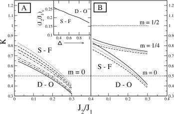
Figure 1: Luttinger liquid parameter ($K$) versus $\frac{J_{2}}{J_{1}}$ for different magnetization state. A constant dashed line at $K=0.5$ is for eye guide line, which separating the spin fluid and dimer order instability state. D-O: dimer order instability state, S-F: spin fluid Luttinger liquid phase. A: Here we only focus at $m=0$ magnetization state. Uppermost (dotted) curve is for $\Delta=0.3$ and the lowermost (solid) curve is for $\Delta=1$. The intermediate curves are for $\Delta=0.4,0.5,0.6.0.8,0.9$ respectively from upper to lower one. Inset shows the separation between the spin fluid and dimer order instability state by a critical line. Here we present the shift of the ${(\frac{J_{2}}{J_{1}})}_{c}$ with $\Delta$. B: Here we present the curves for different magnetization states. $m=1/2$ is independent of $\Delta$ and $\frac{J_{2}}{J_{1}}$ in contrast with $m=1/4,0$. The curves for $m=1/4,0$ plateaus are for $\Delta=0.4,0.5,0.6$ respectively from upper to lower one.

III.1 2.2 Calculations and Results for $m=\frac{1}{4}$ Magnetization States:

Here we discuss the physics of quantum spin pumping of a finite magnetization state. We are considering the magnetization state at $m=\frac{1}{4}$, it corresponds $k_{F}~{}=~{}\pm\frac{\pi}{4}$. The effective Hamiltonian for $J_{2}$ dimerization become,

$$H_{A} = H_{0}~{}-~{}(\frac{{J_{1}}\delta(t)}{2{\pi}^{2}{\alpha}^{2}})~{}\int dx:cos[4\sqrt{K}~{}\phi(x)]:$$ (19)

$$+\frac{A}{2{\pi}^{2}{\alpha}^{2}}~{}\int dx:cos[4\sqrt{K}~{}\phi(x)~{}+~{}\beta]:.$$

Where $A~{}=~{}\sqrt{{{{J_{1}}^{2}}{\Delta}}^{2}~{}+~{}{J_{2}}^{2}}$, ${\beta}~{}=~{}tan^{-1}\frac{{J_{1}}{\Delta}}{J_{2}}$. Apparently it appears from the general derivation of section (II), that the second and third terms of Eq. 19, will be absent due to the oscillatory nature of the integrand but this is not the case when one consider the dimerized lattice. In dimerized lattice, reciprocal lattice vector $G$ will change from $2\pi$ to $\pi$ due to the change of the size of the unit cell. It become more clear, if one write these terms as $~{}\int dx:cos[(G-4k_{F})x~{}+~{}4\sqrt{K}~{}\phi(x)]:$.

Similarly one can write the effective Hamiltonian for $J_{1}$ dimerization:

$$H_{B} = H_{0}~{}+~{}(\frac{{J_{1}}{\Delta}\delta(t)}{2{\pi}^{2}{\alpha}^{2}})~{}\int dx:sin[4\sqrt{K}~{}\phi(x)]:$$ (20)

$$-\frac{A}{2{\pi}^{2}{\alpha}^{2}}~{}\int dx:cos[4\sqrt{K}~{}\phi(x)~{}+~{}\beta]:.$$

The analytical structure of Eq. 19 and Eq. 20 are the same, i.e., the coefficient of the field ${\phi}(x)$ is the same for all sine-Gordon coupling terms. The renormalization group equations for these type of interactions are gia2 ; kos .

$$\frac{dK}{dlnL}~{}=~{}-4{\pi}^{2}K^{2}{\delta(t)}^{2}$$ (21)

$$\frac{d\delta(t)}{dlnL}~{}=~{}(2~{}-~{}4K)\delta(t)$$ (22)

It appears from these RG equations that to get a relevant perturbation, $K$ should be less than $1/2$. It reveals from Fig. 1B that $K$ is exceeding the relevant value in our region of interest to mature criteria for spin pumping. So the dimerization strength should exceed some critical value (${\delta}_{c}$) to initiate the spin pumping phase. These two equations are the Kosterlitz-Thousless equation for the system in this limit. At the critical point, system undergoes Kosterlitz-Thouless transition gia2 ; kos . Since the system flows to the strong coupling (dimer-order) as the dimerization strength exceeds some critical value (${\delta}_{c}$) initially, we have to guess the physics of this phase. We analyze the system in the limit $\delta~{}\rightarrow\pm\infty$ and $K~{}\rightarrow 0$. In this limit all sine-Gordon couplings are relevant but the value of $\phi$ is pinned at the minima of $cos(4\sqrt{K}\phi)$ for NN dimerization and of $sin(4\sqrt{K}\phi)$ for NNN dimerization because the dimerization strength is larger than the other couplings of the system, Hence it produces a deeper minima for the system. This parameter dependent transition, from massless phase to massive phase, at $T=0$ is the quantum phase transition. This quantum phase transition occurs at the every magnetization state. So we conclude that the appearance of quantum spin pumping is not spontaneous like $m=0$, rather dependent on the strength of the parameter.

III.2 2.3 Calculations and Results for $m=\frac{1}{2}$ and Others Fractionally Quantized Magnetization States:

Now we discuss the saturation magnetization at $m=\frac{1}{2}$ ($k_{F}~{}=~{}0$). $K_{F}~{}=~{}0$ implies that the band is empty and the dispersion is not linear, so the validity of the continuum field theory is questionable. Values of the two Luttinger liquid parameters, $v_{0}$ and $K$, are $0$ and $1$ respectively. It also implies that none of the sine-Gordon coupling terms become relevant in this parameter space. So there is no spin pumping for these fractionally quantized magnetization states.

Here we present the explanation for the absence of other fractionally quantized magnetization state (like $1/3,1/5,1/7$ etc): A careful examination of Eq. 12 to Eq. 14 reveals that to get a non oscillatory contribution from Hamiltonian one has to be satisfied $4{k_{F}}=G$ condition but this condition is not fulfilled for these fractionally quantized magnetization state. There are no sine-Gordon coupling terms. Hence there is no spin pumping physics for these fractionally quantized states of magnetization.

IV 3. Conclusions:

We have presented the physics of quantum spin pump for different magnetization state of an antiferomagnetic spin-1/2 chain with competing exchange interactions along with bond-alternation interactions. Our study is completely analytical. We have observed that for some magnetization state spin-pumping is spontaneous and for some other it is not and also explain the physical reasons for the presence and absence of spin pumping for those states.

The author (SS) would like to acknowledge The Center for Condensed Matter Theory of IISc for providing the working space and The National Center for Theoretical Science (Taipei) where the initial phase of this work has started. Finally author thanks, Dr. B. Mukhopadhyay for reading the manuscript very critically.

References

- (1) D. J. Thouless, Phys. Rev. B 27, 6083 (1983).
- (2) Q. Niu. Q and D. J. Thouless, J. Phys. A 17, 2453 (1984).
- (3) P. W. Brouwer, Phys. Rev. B 58, 10135 (1998).
- (4) T. A. Shutenko, I. L. Aleiner and B. L. Altshuler, Phys. Rev. B 61, 10366 (2000).
- (5) Y. Levinson, Entin-O.Wohlman and P. Wolfe, Physica A 302, 335 (2001); Wohlman-O.Entin and A. Aharony, Phys. Rev. B 66, 35329 (2002).
- (6) M. Blaauboer, Phys. Rev. B 65, 235318 (2002).
- (7) J. Wang and B. Wang, Phys. Rev. B 65, 153311 (2002); B. Wang and J. Wang, Phys. Rev. B 66, 201305 (2002).
- (8) P. Sharma and C. Chamon, Phys. Rev. Lett. 87, 96401 (2001); P. Sharma and C. Chamon cond-mat/0209291.
- (9) R. Citro, N. Anderi and Q. Niu, cond-mat/0306181.
- (10) R. Shindou, J. Phys. Soc. Jpn 74, 1214 (2005).
- (11) M. Kohgi , Phys. Rev. Lett 86, 2439 (2001).
- (12) P. Fulde, B. Schmidt and P. Thalmeier, Europhys. Lett 31, 323 (1995).
- (13) Here the system is invariant under the -rotational symmetry which exchange the NN bonds. The direction of electric field and rotational axis are different.
- (14) F. D. M. Haldane, Phys. Rev. B 25, 4925 (1982).
- (15) S. R. White and I. Afflek, Phys. Rev. B 54, 9862 (1996).
- (16) K. Totsuka, Phys. Rev. B 57, 3454 (1998).
- (17) T. Tonegawa Physica B 246-247, 368 (1998).
- (18) S. Chen, H. Buttner and J. Voit, Phys. Rev. Lett 87, 087205 (2001).
- (19) L. Capriotti Phys. Rev. Lett 89, 149701 (2002).
- (20) S. Sarkar and D. Sen, Phys. Rev. B 65, 172408 (2002).
- (21) . field corresponds to the quantum fluctuations (boson) of spin.
- (22) M. V. Berry, Proc. R. Soc. Lond. A 392, 45 (1984).
- (23) J. E. Avron, A. Raveh and B. Zur, Rev. Mod. Phys. 60, 873 (1988); J. E. Avron, J. Berger and Y. Last, Phys. Rev. Lett. 78, 511 (1997).
- (24) R. Chitra, S. Pati, H. R. Krishnamurthy, D. Sen and S. Ramasesha, Phys. Rev. B 52, 6581 (1995).
- (25) Giamarchi. T, Quantum Physics in One Dimension (Oxford Science Publications, Clarendon Press, Oxford, 2004).
- (26) K. Nomura and K. Okamoto, J. Phys. Soc. Jpn. 62, 1123 (1993).
- (27) R. D. Somma and A. A. Aligia, Phys. Rev. B 64, 24410 (2001).
- (28) J. M. Kosterlitz, and D. J. Thouless, J. Phys. C 6, 1181 (1973); V. L. Berezinski, Sov. Phys. JETP 32, 493 (1971).