Density oscillations in multi-component molecular mixtures

Abstract

The excitation spectrum of the density collective oscillations is computed for multi-component molecular mixtures both with Coulomb and (repulsive) short-range interactions. Distinct sound-like excitations appear, governed by the short-range interaction, which differ from the ordinary hydrodynamic sound. The dielectric function and the structure factor are also calculated. The "two-sounds phenomenon" can be understood by means of the predictions of this model.

This paper is motivated by the "two-sounds anomaly" persistently reported over the years in water, either in normal conditions or undercooled,key-1 -key-6 (6) as well as in other liquid molecular mixtures. Inelastic neutron, $X$-ray, Brillouin and, more recently, ultraviolet scattering, either in ordinary or in heavy water, seem to indicate an additional, faster, higher-frequency sound, propagating with velocity $\simeq 3000m/s$ up to intermediate wavevectors (mean inter-molecular distance in water is $\simeq 3\textrm{\AA}$), beside the ordinary hydrodynamic sound propagating with velocity $\simeq 1500m/s$. A dispersionless mode ($\simeq 10^{13}s^{-1}$) was also reported sometimes(key-3, 3),(key-5, 5) (as well as no additional sound(key-7, 7)). The phenomenon is also documented both by simulations of molecular dynamics and experimental data in binary mixtures with large mass difference (metallic alloys, rare-gas mixtures).(key-8, 8)-(key-17, 17)

We show herein that such a "two-sounds anomaly" may appear in interacting molecular systems with (repulsive) short-range interaction. Such a model could reasonably be related to liquid water (or other physical systems as those indicated above). The velocity of the sound-like excitations is independent of temperature, in contrast with the velocity of the hydrodynamic sound which is governed by the adiabatic compressibility, and thus temperature-dependent. In addition, the plasma-like branch of the spectrum due to the Coulomb interaction may appear as another sound-like mode for shorter wavelengths and weak Coulomb coupling. We report here also the computation of the dielectric function and the structure factor within such a model.

We start with the well-known representation of the particle density

$$n(\mathbf{r})=\frac{1}{V}\sum_{i}\delta(\mathbf{r}-\mathbf{r}_{i})=\frac{1}{V}\sum_{\mathbf{q}}e^{i\mathbf{qr}}\sum_{i}e^{-i\mathbf{q}\mathbf{r}_{i}}\,\,\,$$ (1)

for a collection of $N$ particles enclosed in volume $V$, where $\mathbf{r}_{i}$ denotes the position of the $i$-th particle. We consider a small displacement $\mathbf{r}_{i}\rightarrow\mathbf{r}_{i}+\mathbf{u}(\mathbf{r}_{i})$ in these positions, as given by a displacement field $\mathbf{u}(\mathbf{r}_{i})$, such that the particle density becomes

$$\widetilde{n}(\mathbf{r})=\frac{1}{V}\sum_{\mathbf{q}}e^{i\mathbf{qr}}\sum_{i}e^{-i\mathbf{q}\left[\mathbf{r}_{i}+\mathbf{u}(\mathbf{r}_{i})\right]}=\frac{1}{V}\sum_{\mathbf{q}}e^{i\mathbf{qr}}\sum_{i}e^{-i\mathbf{q}\mathbf{r}_{i}}\left[1-i\mathbf{qu}(\mathbf{r}_{i})+...\right]\,\,\,$$ (2)

for $\mathbf{qu}(\mathbf{r}_{i})\ll 1$. Now we employ a Fourier representation

$$\mathbf{u}(\mathbf{r}_{i})=\frac{1}{\sqrt{N}}\sum_{\mathbf{q}}\mathbf{u}(\mathbf{q})e^{i\mathbf{q}\mathbf{r}_{i}}\,\,\,$$ (3)

as well as the well-known random-phase approximation

$$\sum_{i}e^{i(\mathbf{q}-\mathbf{q}^{\prime})\mathbf{r_{i}}}=N\delta_{\mathbf{q},\mathbf{q}^{\prime}}\,\,\,$$ (4)

to get

$$\widetilde{n}(\mathbf{r})=n-in\frac{1}{\sqrt{N}}\sum_{\mathbf{q}}e^{i\mathbf{qr}}\mathbf{qu}(\mathbf{q})\,\,\,,$$ (5)

where $n=N/V$ is the particle density. By comparing equations (1) and (5), we can see that the small change in the density can be represented as

$$\widetilde{n}(\mathbf{r})-n=\delta n(\mathbf{r})=-ndiv\mathbf{u}(\mathbf{r})\,\,\,,$$ (6)

and its Fourier transform $\delta n(\mathbf{q})=-in\mathbf{q}\mathbf{u}(\mathbf{q})$.

We apply this displacement-field approach to a multi-component molecular mixture consisting of several species labelled by $i$, each with $N_{i}$ particles in volume $V$, mass $m_{i}$ and electric charge $ez_{i}$, where $-e$ is the electron charge and $z_{i}$ is a reduced effective charge, interacting through Coulomb potentials $\varphi_{ij}$ and short range potentials $\chi_{ij}$. The mixture is subjected to the neutrality condition $\sum_{i}n_{i}z_{i}=0$, where $n_{i}=N_{i}/V$ is the particle density of the $i$-th species. We consider elementary excitations of the particle density, whose interaction energy is given by

$$U=\frac{1}{2}\sum_{ij}\int d\mathbf{r}d\mathbf{r}^{\prime}\left[\varphi_{ij}(\mathbf{r}-\mathbf{r}^{\prime})+\chi_{ij}(\mathbf{r}-\mathbf{r}^{\prime})\right]\delta n_{i}(\mathbf{r})\delta n_{j}(\mathbf{r}^{\prime})\,\,\,,$$ (7)

where $\varphi_{ij}=e^{2}z_{i}z_{j}/\left|\mathbf{r}-\mathbf{r}^{\prime}\right|$ and $\delta n_{i}(\mathbf{r})$ denotes a small density disturbance which preserves the neutrality. According to equation (6) it can be represented as $\delta n_{i}=-n_{i}div\mathbf{u}_{i}$, where $\mathbf{u}_{i}$ is the displacement field. We use the Fourier transforms

$$\delta n_{i}(\mathbf{r})=\frac{1}{\sqrt{N}}\sum_{\mathbf{q}}\delta n_{i}(\mathbf{q})e^{i\mathbf{qr}}\,\,,\,\,\varphi(\mathbf{r})=\frac{1}{V}\sum_{\mathbf{q}}\varphi(\mathbf{q})e^{i\mathbf{qr}}\,\,\,,$$ (8)

where $N=\sum_{i}N_{i}$ is the total number of particles, $\varphi(\mathbf{r})=e^{2}/r$ and $\varphi(\mathbf{q})=\varphi(q)=4\pi e^{2}/q^{2}$. A similar Fourier transform is employed for the displacement field $\mathbf{u}_{i}$, which leads to $\delta n_{i}(\mathbf{q})=-in_{i}\mathbf{q}\mathbf{u}_{i}(\mathbf{q})$. We can see that only the longitudinal components $u_{i}(\mathbf{q})$ of the displacement field are relevant, so we may write $\mathbf{u}_{i}(\mathbf{q})=(\mathbf{q}/q)u_{i}(\mathbf{q})$, $\delta n_{i}(\mathbf{q})=-iqu_{i}(\mathbf{q})$, with $\delta n_{i}^{*}(-\mathbf{q})$=$\delta n_{i}(\mathbf{q})$, $\mathbf{u}_{i}^{*}(-\mathbf{q})=\mathbf{u}_{i}(\mathbf{q})$ and $u_{i}^{*}(-\mathbf{q})=-u_{i}(\mathbf{q})$. Making use of the Fourier transforms introduced above, the interaction $U$ given by equation (7) can be written as

$$U=-\frac{1}{2n}\sum_{ij\mathbf{q}}n_{i}n_{j}q^{2}\left[\varphi_{ij}(q)+\chi_{ij}(q)\right]u_{i}(\mathbf{q})u_{j}(-\mathbf{q})\,\,\,,$$ (9)

where $\varphi_{ij}(q)=z_{i}z_{j}\varphi(q)$ and $n=N/V$ is the total density of particles. We assume a weak $q$-dependence of $\chi_{ij}(q)$, as for short-range potentials.

Similarly, the kinetic energy associated with the coordinates $u_{i}$ is given by

$$T=-\frac{1}{2n}\sum_{i\mathbf{q}}m_{i}n_{i}\dot{u}_{i}(\mathbf{q})\dot{u}_{i}(-\mathbf{q})\,\,.$$ (10)

In addition, we introduce an external field $\phi(\mathbf{r})$, coupled to the electrical charges, which gives rise to the interaction

$$V=-i\frac{e}{n}\sum_{i\mathbf{q}}n_{i}z_{i}q\phi(\mathbf{q})u_{i}(-\mathbf{q})\,\,.$$ (11)

The equations of motion corresponding to the lagrangian $L=T-U-V$ are given by

$$m_{i}\ddot{u}_{i}+4\pi e^{2}z_{i}\sum_{j}z_{j}n_{j}u_{j}+q^{2}\sum_{j}\chi_{ij}n_{j}u_{j}=-iqez_{i}\phi\,\,\,,$$ (12)

where we dropped out the argument $\mathbf{q}$ in $u_{i}(\mathbf{q})$ and $\phi(\mathbf{q})$ and neglect the weak $q$-dependence of $\chi_{ij}(q)=\chi_{ij}$. In order to simplify these equations we take the same (repulsive) short-range potentials for all species, $\chi_{ij}=\chi>0$, and analyze first the homogeneous system of equations given by (12). We introduce the notations $a=4\pi e^{2}$, $b=q^{2}\chi$,

$$S_{1}=\sum_{i}\frac{z_{i}^{2}n_{i}}{m_{i}}\,\,,\,\,S_{2}=\sum_{i}\frac{n_{i}}{m_{i}}\,\,,\,\,S_{3}=\sum_{i}\frac{z_{i}n_{i}}{m_{i}}\,\,\,,$$ (13)

and

$$x=\frac{1}{n}\sum_{i}z_{i}n_{i}u_{i}\,\,,\,\,y=\frac{1}{n}\sum_{i}n_{i}u_{i}\,\,.$$ (14)

Making use of these notations, the homogeneous system of equations (12) can be written as

$$\begin{array}[]{c}\left(-\omega^{2}+aS_{1}\right)x+bS_{3}y=0\,\,\,,\\ \\ aS_{3}x+\left(-\omega^{2}+bS_{2}\right)y=0\,\,.\end{array}$$ (15)

In addition, we have

$$\omega^{2}u_{i}=\frac{anz_{i}}{m_{i}}x+\frac{bn}{m_{i}}y\,\,.$$ (16)

The spectrum of frequencies $\omega$ of the system of equations (15) can be obtained straightforwardly. It is given by

$$\omega_{1,2}^{2}=\frac{1}{2}\left[aS_{1}+bS_{2}\pm\sqrt{a^{2}S_{1}^{2}+2ab\left(2S_{3}^{2}-S_{1}S_{2}\right)+b^{2}S_{2}^{2}}\right]\,\,.$$ (17)

The $\omega_{1}$-branch in equation (17) (corresponding to the plus sign) represents the plasmonic excitations. In the long wavelength limit it reads

$$\omega_{1}^{2}=aS_{1}+bS_{3}^{2}/S_{1}=\omega_{p}^{2}+bS_{3}^{2}/S_{1}\,\,\,,\,\,\,q\rightarrow 0\,\,\,,$$ (18)

where $\omega_{p}$, given by

$$\omega_{p}^{2}=aS_{1}=4\pi e^{2}\sum_{i}\frac{z_{i}^{2}n_{i}}{m_{i}}\,\,\,,$$ (19)

is the plasma frequency. For shorter wavelengths the $\omega_{1}$-branch approaches an asymptote given by

$$\omega_{1}^{2}\simeq bS_{2}+aS_{3}^{2}/S_{2}\,\,\,,\,\,\,q\rightarrow\infty.$$ (20)

The $\omega_{2}$-branch in equation (17) (corresponding to the minus sign) represents sound-like excitations. In the long wavelength limit it is given by

$$\omega_{2}^{2}=\left(S_{2}-S_{3}^{2}/S_{1}\right)b=v_{s}^{2}q^{2}\,\,\,,\,\,\,q\rightarrow 0\,\,\,,$$ (21)

where

$$v_{s}=\sqrt{\left(S_{2}-S_{3}^{2}/S_{1}\right)\chi}\,\,\,$$ (22)

is the corresponding sound velocity. We can see easily, by applying the Schwarz-Cauchy inequality to the vectors $a_{i}=\sqrt{n_{i}/m_{i}}$ and $b_{i}=z_{i}\sqrt{n_{i}/m_{i}}$, that $v_{s}^{2}$ is always positive ($(S_{2}-S_{3}^{2}/S_{1})\geq 0$). For shorter wavelengths the $\omega_{2}$-branch of the spectrum approaches an horizontal asymptote given by

$$\omega_{2}^{2}\simeq\left(1-S_{3}^{2}/S_{1}S_{2}\right)\omega_{p}^{2}\,\,\,,\,\,\,q\rightarrow\infty\,\,.$$ (23)

In the limit of vanishing Coulomb coupling ($a\rightarrow 0$) the sound-branch of the spectrum becomes $\omega_{2}^{2}=bS_{2}=v_{s}^{2}q^{2}$, where

$$v_{s}^{2}=\chi S_{2}=\chi\sum_{i}(n_{i}/m_{i})\,\,\,,$$ (24)

an expression which holds also for the same mass $m_{i}=m$ for all particles (one component), due to the neutrality condition ($S_{3}=0$).

The above elementary excitations, which are governed by interaction, are non-equilibrium collective modes which might be termed density "kinetic" modes.(key-18, 18) The sound-like excitations ($\omega_{2}$-branch in equation (17)) may be called "densitons", in order to distinguish them from plasmons ($\omega_{1}$-branch in equation (17)) and from the ordinary sound. They may correspond to the density collective modes suggested by Zwanzig for classical liquids.(key-19, 19) We emphasize that these sound-like excitations are distinct from the ordinary hydrodynamic sound.

Indeed, the interaction corresponding to the latter can be written as

$$U=\frac{1}{2\kappa}\int d\mathbf{r}\left[div\mathbf{u}(\mathbf{r})\right]^{2}=-\frac{1}{2\kappa n}\sum_{\mathbf{q}}q^{2}u(\mathbf{q})u(-\mathbf{q})\,\,\,,$$ (25)

where $\kappa=-(1/V)(\partial V/\partial p)_{S}$ is the adiabatic compressibility ($p$ denotes the pressure and $S$ stands for entropy). The above equation is derived by making use of the change $\delta V=-V(\delta n/n)=Vdiv\mathbf{u}$ in volume. We emphasize that for thermodynamic equilibrium we have only one displacement field $\mathbf{u}(\mathbf{r})$. Equation (25) together with the kinetic energy given by equation (10) for $u_{i}(\mathbf{q})=u(\mathbf{q})$ leads to the sound branch $\omega_{0}^{2}=v_{0}^{2}q^{2}$, corresponding to the ordinary sound propagating with a velocity $v_{0}$ given by

$$v_{0}^{2}=\left(\kappa\sum_{i}n_{i}m_{i}\right)^{-1}\,\,.$$ (26)

For $m_{i}=m$ (one component) the above equation gives the well-known velocity $v_{0}=1/\kappa nm$ of the ordinary sound. As it is well-known, it has a slight temperature dependence, through the compressibility, in contrast with the velocity $v_{s}$ given above for the sound-like excitations. For an electrically neutral multi-component mixture it can be shown easily that $v_{s}^{2}/v_{0}^{2}\geq n^{2}\chi\kappa$.

If we apply equations (24) and $(\ref{26})$ to both ordinary and heavy water (one component, neutral molecule), and assume that interaction $\chi$ and, respectively, the compressibility $\kappa$ are the same for the two kinds of water, we can see that the two sound velocities $v_{s}$ and $v_{0}$ exhibit a slight isotopic effect, while their ratio $v_{s}/v_{0}=n\sqrt{\chi\kappa}$ does not exhibit such an isotopic effect, in agreement with experimental data. In this case we may take $v_{0}=1500m/s$ and $v_{s}=3000m/s$ from experimental data and get the interaction parameter $\chi\simeq 60eV\cdot\textrm{\AA}^{3}$ (for a mean inter-molecular spacing $\simeq 3\textrm{\AA}$) . A similar picture, given by equations (24) and (26), may apply to rare-gas mixtures, while for metallic alloys the Coulomb coupling must be taken into account (and equation (22) employed).

If we assume the existence of a dispersionless mode in water, then we may consider that water molecule is dissociated to some extent, and its components have an electric charge, such that the plasmonic mode given by equation (19) can be identified with such a dispersionless mode. Various models of dissociation of the water molecule are known, like $OH^{-}-H^{+}$ or $OH^{-}-H_{3}O^{+}$. In all cases a certain mobility of the $H^{+}$ (hydrogen) cations and $O^{-}$ (oxygen) anions is implied. We assume here that the dynamics of liquid water has a plasma-like component consisting of $H^{+z}$ cations with density $2n$ and mass $m$ (proton mass) and $O^{-2z}$ anions with density $n$ and mass $M=16m$, where $n$ is the density of water. The excitation spectrum given by equations (17) for such an $O^{-2z}-H^{+z}$ plasma is shown in Fig. 1.

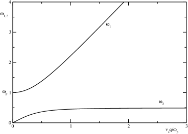
Figure 1: Spectrum of density excitations given by equation (17) for the $O^{-2z}-H^{+z}$ plasma.

Taking $\omega=10^{13}s^{-1}$($\simeq 5meV$) of the dispersionless mode(key-3, 3),(key-5, 5),(key-7, 7) as the plasma frequency $\omega_{p}$ given by $\omega_{p}^{2}=16\pi ne^{2}z^{2}/\mu$ (equation (19)), where $\mu=2mM/(M+2m)$ is the reduced mass, we get $z\simeq 3\times 10^{-2}$. The velocity of the hydrodynamic sound is given by $v_{0}=1/\sqrt{\kappa n(M+2m)}$ according to equation (26) and the velocity of the sound-like excitations is given by $v_{s}=\sqrt{9n\chi/(M+2m)}$ from equation (22). We can see that both velocities exhibit an isotopic effect, but their ratio $v_{s}/v_{0}=3n\sqrt{\chi\kappa}$ does not, in agreement with the experimental data. From $v_{s}=3000m/s$ we derive the interaction $\chi\simeq 7eV\cdot\textrm{\AA}^{3}$. Similar results are obtained for other forms of dissociation, like $OH^{-}-H^{+}$ or $OH^{-}-H_{3}O^{+}$. In this respect, the $O^{-2z}-H^{+z}$ plasma model can be viewed as an average, effective model for various plasma components that may exist in water.

According to equation (20), for shorter wavelengths the $\omega_{1}$-branch approaches an asymptote given by $\omega_{1}^{2}\sim bS_{2}+aS_{3}^{2}/S_{2}$. In the limit of weak Coulomb coupling this $\omega_{1}$-branch may appear as an "anomalous" sound given by

$$\omega_{a}=\sqrt{bS_{2}}=v_{a}q\,\,\,,$$ (27)

propagating with velocity

$$v_{a}=\sqrt{S_{2}\chi}=\frac{1}{\sqrt{1-S_{3}^{2}/S_{1}S_{2}}}v_{s}\,\,\,$$ (28)

(which is always a positive qauntity). This additional, anomalous sound is always faster than the sound-like excitations propagating with velocity $v_{s}$, since

$$\frac{v_{a}}{v_{s}}=\frac{1}{\sqrt{1-S_{3}^{2}/S_{1}S_{2}}}>1\,\,.$$ (29)

It is worth noting that the molecular dynamics studies which originary predicted such a fast, anomalous sound(key-20, 20) employed indeed a Coulomb interaction and a short-range one. We note, however, that the velocity $v_{a}$ as given by (28) does not depend on the Coulomb coupling. In the plasma model for water discussed above the ratio $v_{a}/v_{0}$ is approximately $2$ ($\simeq\sqrt{2M/9m+5/9}$), but it exhibits an isotopic effect, which does not seem to be supported by the experimental data.

It is easy to derive the dielectric function in the limit of long wavelengths from equation (12). Indeed, for charged particles equation $\delta n_{i}=-n_{i}div\mathbf{u}_{i}$ is equivalent with Maxwell equation $div\mathbf{E}_{i}=4\pi q_{i}\delta n_{i}$, where the electric field is given by $\mathbf{E}_{i}=-4\pi q_{i}n_{i}\mathbf{u}_{i}$ and $q_{i}=ez_{i}$ is the electric charge of the $i$-th species. It follows that the internal field is given by

$$E_{int}=-4\pi e\sum_{i}z_{i}n_{i}u_{i}\,\,$$ (30)

We get easily this field from equations (12),

$$E_{int}=-iq\phi\frac{\omega_{p}^{2}}{\omega^{2}-\omega_{p}^{2}}\,\,\,$$ (31)

in the long wavelength limit (it is proportional to $x$ given by equation (14)). The dielectric function is defined by $D=\varepsilon E=\varepsilon(D+E_{int})$, where $D=-iq\phi$ is the external field (electric displacement). We get the plasma dielectric function

$$\varepsilon=1-\omega_{p}^{2}/\omega^{2}\,\,\,,$$ (32)

as expected. It exhibits an absorption edge ($\omega_{p}$) for very low frequencies. In the static limit it is reasonable to admit the existence of an additional internal field of intrinsic polarizability which removes the $\omega=0$ singularity.

We pass now to the calculation of the structure factor. From equation (16) we can see that the displacement $u_{i}$ is a superposition of the two eigenvectors of the system of equations (15), which oscillate with eigenfrequencies $\omega_{1,2}$, respectively. It follows that these coordinates are those of linear harmonic oscillators with the potential energy of the form $m_{i}\omega^{2}u_{i}^{2}/2$. The statistical distribution of the coordinates $u_{i}$ in the classical limit is given by $dw\sim\exp(-m_{i}\omega^{2}u_{i}^{2}/2T)du_{i}$, where $T$ denotes the temperature. We get the thermal averages

$$\left\langle u_{i}u_{j}\right\rangle=\frac{T}{m_{i}\omega^{2}}\delta_{ij}\,\,.$$ (33)

On the other hand the structure factor defined by

$$\begin{array}[]{c}S(q,\omega)=\frac{1}{2\pi}\int d\mathbf{r}d\mathbf{r}^{\prime}dt\left\langle\delta n(\mathbf{r},t)\delta n(\mathbf{r}^{\prime},0)\right\rangle e^{i\mathbf{q}(\mathbf{r}-\mathbf{r}^{\prime})-i\omega t}=\\ \\ =\frac{N}{2\pi n^{2}}\int dt\left\langle\delta n(\mathbf{q},t)\delta n(-\mathbf{q},0)\right\rangle e^{-i\omega t}\end{array}$$ (34)

(we leave aside the central peak) can be written as

$$S(q,\omega)=\frac{Nq^{2}}{2\pi n^{2}}\int dt\sum_{ij}n_{i}n_{j}\left\langle u_{i}(t)u_{j}(0)\right\rangle e^{-i\omega t}\,\,.$$ (35)

Writing

$$u_{i}=u_{i}^{(1)}e^{i\omega_{1}t}+u_{i}^{(2)}e^{i\omega_{2}t}\,\,\,$$ (36)

and making use of equation (33) we get the structure factor

$$S(q,\omega)=NTq^{2}\left(\sum_{i}n_{i}^{2}/n^{2}m_{i}\right)\left[\frac{1}{\omega_{1}^{2}}\delta(\omega-\omega_{1})+\frac{1}{\omega_{2}^{2}}\delta(\omega-\omega_{2})\right]\,\,.$$ (37)

We can see that the relevant sound contributions read

$$S(q,\omega)\simeq\frac{NT}{v_{s,a}^{2}}\left(\sum_{i}n_{i}^{2}/n^{2}m_{i}\right)\delta(\omega-v_{s,a}q)\,\,.$$ (38)

The relaxation and damping effects can be included in the above expressions of the structure factor. As it is well-known, they amount to representing the $\delta$-functions by lorentzians.

The short-range interaction $\chi$ can be generalized to an interaction matrix $\chi_{ij}$ with distinct elements for each pair of species. In this case, the excitation spectrum of the density oscillations may exhibit multiple branches in general, for a multi-component mixture. In addition, it may have special features, like a dip in the plasmonic branch, or negative velocity for the sound-like excitations, which may indicate either an anomalous behaviour or unphysical situations, depending on the mutual magnitudes of the short-range potentials $\chi_{ij}$.

Now it is worthwhile commenting upon the validity of the approach presented above. If we keep higher-order terms in the expansion given by equation (2) (i.e. for moderate values of $\mathbf{q}\mathbf{u}_{i}$) then additional interactions appear in equation (9), which leads to finite lifetimes for the density excitations. This means that for larger wavevectors $\mathbf{q}$ these excitations are not anymore well-defined excitations, as expected. Making use of equation (33) we can estimate the mean product $qu_{i}$ for the sound-like branch as $qu_{i}\sim\sqrt{T/m_{i}v_{s}^{2}}$ , where the velocity $v_{s}$ is given by equation (22). This gives rather small values for $qu_{i}$. For instance, for water we get $qu\sim 0.5$ (at room temperature), which shows that the wavevector $q$ may take reasonable large values providing the displacement $u$ is sufficiently small. For the plasmonic branch, the condition $qu_{i}\ll 1$ gives a cutoff wavevector $q_{c}^{i}\simeq\sqrt{m_{i}\omega_{p}^{2}/T}$ for large $\omega_{p}$; for small values of the plasma frequency the condition becomes $qu_{i}\sim\sqrt{T/m_{i}v_{a}^{2}}\ll 1$.

Another source of finite lifetime for the density excitations arises from the kinetic term. Indeed, under the displacement $\mathbf{r}_{ik}\rightarrow\mathbf{r}_{ik}+\mathbf{u}_{i}(\mathbf{r}_{ik})$, where $\mathbf{r}_{ik}$ is the position of the $k$-th particle in the $i$-th species, a mixed term

$$H_{int}=\sum_{ik}m_{i}\mathbf{v}_{ik}\dot{\mathbf{u}}_{i}(\mathbf{r}_{ik})\,\,\,$$ (39)

appears in the kinetic term, where $\mathbf{v}_{ik}=\dot{\mathbf{r}}_{ik}$ is the velocity of the $ik$-particle. It is easy to get an upper bound for this term, by using the Schwarz-Cauchy inequality. It is given by $N\left\langle m_{i}v_{ik}^{2}\right\rangle^{1/2}\left\langle m_{i}\dot{u}_{i}^{2}\right\rangle^{1/2}$ or, by making use of (33), $\sqrt{\varepsilon T}$ per particle, where $\varepsilon$ represents the mean kinetic energy (which depends on temperature, in principle). This estimation can be taken as an uncertainty in energy, leading to a lifetime $\tau\simeq\hbar/\sqrt{\varepsilon T}$ and a corresponding meanfree path $\Lambda=v_{s}\tau$ for the sound-like excitations. For wavelengths $\lambda$ much longer than the meanfree path, i.e. for wavevectors $q$ such as $q\ll 1/v_{s}\tau$ we are in the collision-like regime ($\omega_{2}\tau\ll 1$), and the collisions can establish the thermodynamic equilibrium (hydrodynamic regime). In this case the ordinary sound can be propagated (with velocity $v_{0}$). For $q\gg 1/v_{s}\tau$ we are in the collisionless regime, the ordinary sound is absorbed, and the non-equilibrium sound-like excitations ("densitons") can be propagated (with velocity $v_{s}$). Unfortunately, it is difficult to have a reliable estimation of the energy $\varepsilon$, and so of the threshold wavevector $q_{t}=1/v_{s}\tau=\sqrt{\varepsilon T}/\hbar v_{s}$. For $\varepsilon=10meV$ (and $v_{s}=3000m/s$, $T=300K$) we get $q_{t}\simeq 0.1\textrm{\AA}^{-1}$, which is in a reasonable order-of-magnitude agreement with the experimental data.(key-1, )-(key-6, 6),(key-11, 11),(key-12, 12),(key-15, 15) It is interesting to note that if we apply this estimation to weakly-interacting gases, where we may take $\varepsilon\sim T$, we get a high value of the threshold wavevector $q_{t}\sim T/\hbar v_{s}$, since $v_{s}$ is very small (the short-range interaction is weak). We may say that in gases there is very unlikely to exist the sound-like excitations; it is only the ordinary sound that exists. On the contrary, the collision-like regime is quite unlikely in ordinary solids, so we have there sound-like excitations and to a much lesser extent ordinary sound.

Finally, we note that the collective excitations derived above contribute to the thermodynamics of liquids. Indeed, the free energy can be written as

$$F=F_{0}+F_{1}+F_{2}=F_{0}+T\sum_{\mathbf{q}}\ln\left(1-e^{-\hbar\omega_{1}/T}\right)+T\sum_{\mathbf{q}}\ln\left(1-e^{-\hbar\omega_{2}/T}\right)\,\,\,,$$ (40)

where $F_{0}$ is the free energy associated with the particle movements and $\omega_{1,2}$ are given by equation (17). The evaluation of integrals in equation (40) depends on the particular magnitude of the excitation spectrum, but usually the integrals are rapidly convergent and their contribution to the thermodynamic properties of the liquid is small. For instance, the sound-like contribution is approximately given by $F_{2}\simeq-\pi^{2}VT(T/\hbar v_{s})^{3}/90$, which is indeed a small correction to $F_{0}$ (the latter being governed mainly by the liquid cohesion).

In conclusion, we have shown that in interacting molecular systems there may appear sound-like excitations controlled by short-range interactions, distinct from the ordinary hydrodynamic sound. The former are non-eequilibrium excitations, while the latter appear through equilibrium, adiabatic processes. The velocity $v_{s}$ of the sound-like excitations is independent of temperature, while the velocity $v_{0}$ of the ordinary sound depends on temperature, through the adiabatic compressibility. In order to distinguish them we propose to call the former "kinetic" modes of particle density, or "densitons". In addition, in the presence of Coulomb interaction, the well-known plasmonic branch is present in the spectrum of the density excitations, which, for shorter wavelengths and weak Coulomb coupling may look like another, anomalous, fast sound. We have shown that the "two-sounds anomaly" reported in liquids like water, rare-gas mixtures, metallic alloys, etc, and documented by molecular dynamics studies, can be understood on this basis.

References

(1)J. Teixeira, M. C. Bellissent-Funel, S. H. Chen and
B. Dorner, Phys. Rev. Lett. 54 2681 (1985).
(2)F. Sette, G. Ruocco, M. Krish, U. Bergmann, C.
Masciovecchio, V. Mazzacurati, G. Signorelli and R. Verbeni, Phys.
Rev. Lett. 75 850 (1995).
(3)F. Sette, G. Ruocco, M. Krisch, C. Masciovecchio,
R. Verbeni and U. Bergmann, Phys. Rev. Lett. 77 83 (1996).
(4)G. Ruocco and F. Sette, J. Phys. Cond. Matt. 11
R259 (1999).
(5)C. Petrillo, F. Sacchetti, B. Dorner and J.-B.
Suck, Phys. Rev. E62 3611 (2000).
(6)S. C. Santucci, D. Fioretto, L. Comez, A. Gessini
and C. Masciovecchio, Phys. Rev. Lett. 97 225701 (2006).
(7)F. J. Bermejo, M. Alvarez, S. M. Bennington and
R. Vallauri, Phys. Rev. E51 2250 (1995).
(8)J. Bosse, G. Jacucci, M. Ronchetti and W. Schirmacher,
Phys. Rev. Lett. 57 3277 (1986).
(9)M. A. Ricci, D. Rocca, G. Ruocco and R. Vallauri,
Phys. Rev. Lett. 61 1958 (1988).
(10)M. A. Ricci, D. Rocca, G. Ruocco and R. Vallauri,
Phys. Rev. A40 7226 (1989).
(11)W. Montfrooij, P. Westerhuijs, V. O. de Haan
and I. M. de Schepper, Phys. Rev. Lett. 63 544 (1989).
(12)U. Balucani, G. Ruocco, A. Torcini and R. Vallauri,
Phys. Rev. E47 1677 (1993).
(13)F. Sciortino and S. Sastry, . J. Chem. Phys.
100 3881 (1994).
(14)M. Sampoli, G. Ruocco and F. Sette, Phys. Rev.
Lett. 79 1678 (1997).
(15)M. Alvarez, F. J. Bermejo, P. Verkerk and B.
Roessli, Phys. Rev. Lett. 80 2141 (1998).
(16)E. Enciso, N. G. Almarza, M. A. Gonzalez, F.
J. Bermejo, R. Fernandez-Perea and F. Bresme, Phys. Rev. Lett. 81
4432 (1998).
(17)M. Sampoli, U. Bafile, E. Guarini and F. Barocchi,
Phys. Rev. Lett. 88 085502 (2002).
(18)See, for instance, A. Campa and E. G. D. Cohen,
Phys. Rev. Lett. 61 853 (1988).
(19)R. Zwanzig, Phys. Rev. 156 190 (1967).
(20)A. Rahman and F. H. Stilllinger, Phys. Rev. A10
368 (1974).