Abstract

We derive a sufficient condition for the existence of index-guided modes in a very general class of dielectric waveguides, including photonic-crystal fibers (arbitrary periodic claddings, such as “holey fibers”), anisotropic materials, and waveguides with periodicity along the propagation direction. This condition provides a rigorous guarantee of cutoff-free index-guided modes in any such structure where the core is formed by increasing the index of refraction (e.g. removing a hole). It also provides a weaker guarantee of guidance in cases where the refractive index is increased “on average” (precisely defined). The proof is based on a simple variational method, inspired by analogous proofs of localization for two-dimensional attractive potentials in quantum mechanics.

OCIS codes: (060.5295) Photonic crystal fibers; (130.2790) Guided waves; (060.2310) Fiber optics; (060.4005) Microstructured fibers.

1 Introduction

In this paper, we present rigorous sufficient conditions for the existence of index-guided modes, including conditions for cutoff-free modes, in a wide variety of dielectric waveguides—from ordinary step-index fibers [1], to photonic-crystal “holey” fibers [2, 3, 4, 5], and even fiber-Bragg gratings [6] or other periodically modulated waveguides [7, 8, 5]. The dispersion relations of such waveguides must almost always be computed numerically, and so exact analytical theorems like the one derived here provide a foundation of certainty that is not available in any other way. A rigorous theorem allows us to give a general answer (although not a necessary condition) for questions such as: if the waveguide core has a mixture of higher- and lower-index regions, how much higher-index material is enough for cutoff-free guidance; and under what conditions do photonic-crystal fibers, like step-index fibers, have cutoff-free guided modes? The theorem provides an absolute guarantee, with no calculation required, that strictly increasing the refractive index to form the waveguide (e.g. filling in a hole of a holey fiber) yields a cutoff-free guided mode. It also leads directly to necessary conditions for single-polarization fibers, the subject of another manuscript currently in prepration. Our work extends an earlier proof of guided modes for homogeneous-cladding, non-periodic, dielectric waveguides with isotropic [9] or anistropic [10] materials, and is closely related in spirit to proofs of the existence of bound modes in two-dimensional potentials for quantum mechanics [11].

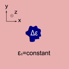
(a) Cross section of a waveguide (e.g. a conventional fiber) with a homogeneous cladding and an arbitrary-shape core.

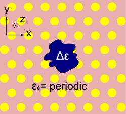
(b) Cross section of a photonic-crystal fiber with periodic cladding and arbitrary-shape core.

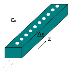
(c) A waveguide periodic in the propagation ($z$) direction surrounded by a homogenous cladding.

Fig. 1: Schematics of various types of dielectric waveguides in which our theorem is applicable. Light propagates in the $z$ direction (along which the structure is either uniform or periodic) and is confined in the $xy$ direction by a higher-index core compared to the surrounding (homogeneous or periodic cladding).

The most common guiding mechanism in dielectric waveguides is index guiding (or “total internal reflection”), in which a higher-index core is surrounded by a lower-index cladding $\varepsilon_{c}$ ($\varepsilon$ is the relative permittivity, the square of the refractive index in isotropic non-magnetic materials). A schematic of several such dielectric waveguides is shown in Fig. 1. In particular, we suppose that the waveguide is described by a dielectric function $\varepsilon(x,y,z)=\varepsilon_{c}(x,y,z)+\Delta\varepsilon(x,y,z)$ such that: $\varepsilon$, $\varepsilon_{c}$, and $\Delta\varepsilon$ are periodic in $z$ (the propagation direction) with period $a$ ($a\to 0$ for the common case of a waveguide with a constant cross-section); that the cladding dielectric function $\varepsilon_{c}$ is periodic in $xy$ (e.g. in a photonic-crystal fiber), with a homogeneous cladding (e.g. in a conventional fiber) as a special case; and the core is formed by a change $\Delta\varepsilon$ in some region of the $xy$ plane, sufficiently localized that $\int|1/\varepsilon-1/\varepsilon_{c}|<\infty$ (integrated over the $xy$ plane and the unit cell in $z$). This includes a very wide variety of dielectric waveguides, from conventional fibers [Fig. 1(a)] to photonic-crystal “holey” fibers [Fig. 1(b)] to waveguides with a periodic “grating” along the propagation direction [Fig. 1(c)] such as fiber-Bragg gratings and other periodic waveguides. We exclude metallic structures (i.e, we require $\varepsilon>0$) and make the approximation of lossless materials (real $\varepsilon$). We allow anisotropic materials. The case of substrates (e.g. for strip waveguides in integrated optics [12, 13, 14]) is considered in Sec. 5. We also consider only non-magnetic materials (relative permeability $\mu=1$), although a future extension to magnetic materials should be straightforward. Intuitively, if the refractive index is increased in the core, i.e. if $\Delta\varepsilon$ is non-negative, then we might expect to obtain exponentially localized index-guided modes, and this expectation is borne out by innumerable numerical calculations, even in complicated geometries like holey fibers [2, 3, 4, 5].

However, an intuitive expectation of a guided mode is far from a rigorous guarantee, and upon closer inspection there arise a number of questions whose answers seem harder to guess with certainty. First, even if $\Delta\varepsilon$ is strictly non-negative, is there a guided mode at every wavelength, or is there the possibility of e.g. a long-wavelength cutoff (as was initially suggested in holey fibers [15], but was later contradicted by more careful numerical calculations [16])? Second, what if $\Delta\varepsilon$ is not strictly non-negative, i.e. the core consists of partly increased and partly decreased index; it is known in such cases, e.g. in “W-profile fibers” [17] that there is the possibility of a long-wavelength cutoff for guidance, but precisely how much decreased-index regions does one need to have such a cutoff? Third, under some circumstances it is possible to obtain a “single-polarization” fiber, in which the waveguide is truly single-mode (as opposed to two degenerate polarization modes as in a cylindrical fiber) [18, 19, 20, 21, 22, 23]—our theorem can be extended, similar to Ref. 9, to a condition for two guided modes, and we will explore the consequences for single-polarization fibers in a subsequent paper. It turns out that all of these questions can be rigorously answered (in the sense of sufficient conditions for guidance) for the very general geometries considered in Fig. 1, without resorting to approximations or numerical computations.

We will proceed as follows. First, in Sec. 2, we review the mechanism of index guiding, state our result (a sufficient condition for the existence of index-guided modes), and discuss some important special cases. In Sec. 3, we first prove this theorem for the simplified special case of a homogeneous cladding $\varepsilon_{c}$, where the proof is much easier to follow. Then, in Sec. 4, we generalize the proof to arbitrary periodic claddings, such as for holey photonic-crystal fibers (with some algebraic details left to the appendix). In Sec. 5, we discuss a few contexts that go beyond the initial assumptions of our theorem: substrates, material dispersion, and finite-size effects. Finally, we offer some concluding remarks in Sec. 6 discussing future directions.

2 Statement of the theorem

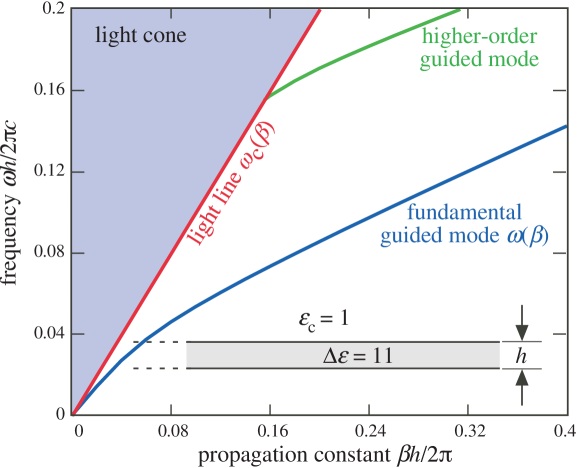
Fig. 2: Example dispersion relation of a simple 2d dielectric waveguide in air (inset) for the TM polarization (electric field out of the plane), showing the light cone, the light line, the fundamental (cutoff-free) guided mode, and a higher-order guided mode with a cutoff.

First, let us review the basic description of the eigenmodes of a dielectric waveguide [1, 5]. In a waveguide as defined above, the solutions of Maxwell’s equations (both guided and non-guided) can be written in the form of eigenmodes $\mathbf{H}(x,y,z)e^{i\beta z-i\omega t}$ (via Bloch’s theorem thanks to the periodicity in $z$) [5], where $\omega$ is the frequency, $\beta$ is the propagation constant, and the magnetic-field envelope $\mathbf{H}(x,y,z)$ is periodic in $z$ with period $a$ (or is independent of $z$ in the common case of a constant cross section, $a\to 0$). A plot of $\omega$ versus $\beta$ for all eigenmodes is the “dispersion relation” of the waveguide, one example of which is shown in Fig. 2. In the absence of the core (i.e. if $\Delta\varepsilon=0$), the (non-localized) modes propagating in the infinite cladding form the “light cone” of the structure [2, 3, 4, 5]; and at each real $\beta$ there is a fundamental (minimum-$\omega$) space-filling mode at a frequency $\omega_{c}(\beta)$ with a corresponding field envelope $\mathbf{H}_{c}$ [2, 3, 4, 5]. Such a light cone is shown as a shaded triangular region in Fig. 2. Below the “light line” $\omega_{c}(\beta)$, the only solutions in the cladding are evanescent modes that decay exponentially in the transverse directions [24, 2, 3, 4, 5]. Therefore, once the core is introduced ($\Delta\varepsilon\neq 0$), any new solutions with $\omega<\omega_{c}$ must be guided modes, since they are exponentially decaying in the cladding far from the core: these are the index-guided modes (if any). Such guided modes are shown as lines below the light cone in Fig. 2: in this case, both a lowest-lying (“fundamental”) guided mode with no low-frequency cutoff (although it approaches the light line asymptotically as $\omega\to 0$) and a higher-order guided mode with a low-frequency cutoff are visible. Since a mode is guided if $\omega<\omega_{c}$, we will prove the existence of a guided mode by showing that $\omega$ has an upper bound $<\omega_{c}$, using the variational (minimax) theorem for Hermitian eigenproblems [5].

[Modes that lie beneath the light light are not the only type of guided modes in microstructured dielectric waveguides. While all the guided modes in a traditional, homogeneous-cladding fiber lie below the light line and are confined by the mechanism of index-guiding, there can also be bandgap-guided modes in photonic-crystal fibers [2, 3, 4, 5]. These bandgap-guided modes lie above the cladding light line and are therefore not index-guided. Bandgap-guided modes always have a low-frequency cutoff (since in the long-wavelength limit the structure can be approximated by a “homogenized” effective medium that has no gap [25]). We do not consider bandgap-guided modes in this work; sufficient conditions for such modes to exist were considered by Ref. 26.]

We will derive the following sufficient condition for the existence of an index-guided mode in a dielectric waveguide at a given $\beta$: a guided mode must exist whenever

$$\int\mathbf{D}_{c}^{*}\cdot\left(\varepsilon^{-1}-\varepsilon_{c}^{-1}\right)\mathbf{D}_{c}<0,$$ (1)

where the integral is over $xy$ and one period in $z$ and $\mathbf{D}_{c}$ is the displacement field of the cladding’s fundamental mode. From this, we can immediately obtain a number of useful special cases:

• There must be a cutoff-free guided mode if $\Delta\varepsilon\geq 0$ everywhere (i.e., if we only increase the index to make the core).

• For a homogeneous cladding (and isotropic media), there must be a cutoff-free guided mode if $\int(1/\varepsilon-1/\varepsilon_{c})<0$ (similar to the earlier theorem of Ref. 9, but generalized to include waveguides periodic in $z$ and/or cores $\Delta\varepsilon$ that do not have compact support).

• More generally, a guided mode has no long-wavelength cutoff if eq. (1) is satisfied for the quasi-static ($\omega\to 0$, $\beta\to 0$) limit of $\mathbf{D}_{c}$.

Equation (1) can also be extended to a sufficient condition for having two guided modes (or equivalently, a necessary condition for single-polarization guidance), when the cladding fundamental mode is doubly degenerate. We explore this generalization, analogous to a result in Ref. 9 for homogeneous claddings, in another manuscript currently being prepared.

3 Waveguides with a homogeneous cladding

To illustrate the basic ideas of the proof in a simpler context, we will first consider the case of a homogeneous cladding ($\varepsilon_{c}=\mathrm{constant}$) and isotropic, $z$-invariant strucures ($\varepsilon$ is a scalar function of $x$ and $y$ only). In doing so, we reproduce a result first proved (using a somewhat different approach) by [9] (although the latter result required $\Delta\varepsilon$ to have compact support, whereas we only require a weaker integrability condition). Our proof, which we generalize in the next section, is closely inspired by a proof [11] of a related result in quantum mechanics, the fact that any attractive potential in two dimensions localizes a bound state [27, 28, 29, 11, 30]; we discuss this analogy in more detail below.

That is, we take the dielectric function $\varepsilon(x,y)$ to be of the form:

$$\varepsilon(x,y)=\varepsilon_{c}+\Delta\varepsilon(x,y),$$ (2)

where $\Delta\varepsilon$ is an an arbitrary change in $\varepsilon$ that forms the core of the waveguide. For convenience, we define a new function $\Delta$ by:

$$\Delta(x,y)\triangleq\varepsilon^{-1}-\varepsilon_{c}^{-1}.$$ (3)

The only constraints we place on $\Delta\varepsilon$ are that $\varepsilon$ be real and positive and that $\int|\Delta|dxdy$ be finite, as discussed above. Now, we wish to show that there must always be a (cutoff-free) guided mode as long as $\Delta\varepsilon$ is “mostly positive,” in the sense that:

$$\int\Delta(x,y)\,dxdy<0,$$ (4)

Since eq. (4) is independent of $\omega$ or $\beta$, the existence of guided modes will hold at all frequencies (cutoff-free).

The foundation for the proof is the existence of a variational (minimax) theorem that gives an upper bound for the lowest eigenfrequency $\omega_{\mathrm{min}}$. In particular, at each $\beta$, the eigenmodes $\mathbf{H}(x,y)e^{i\beta z-i\omega t}$ satisfy a Hermitian eigenproblem [5]:

$$\nabla_{\beta}\times\frac{1}{\varepsilon}\nabla_{\beta}\times\mathbf{H}=\hat{\Theta}_{\beta}\mathbf{H}=\frac{\omega^{2}}{c^{2}}\mathbf{H},$$ (5)

where

$$\nabla_{\beta}\triangleq\nabla+i\beta\hat{\mathbf{z}},$$ (6)

with eq. (5) defining the linear operator $\hat{\Theta}_{\beta}$. In addition to the eigenproblem, there is also the “transversality” constraint [24, 5]:

$$\nabla_{\beta}\cdot\mathbf{H}=0$$ (7)

(the absence of static magnetic charges). From the Hermitian property of $\hat{\Theta}_{\beta}$, the variational theorem immediately follows [5]:

$$\frac{\omega_{\mathrm{min}}^{2}(\beta)}{c^{2}}=\inf_{\nabla_{\beta}\cdot\mathbf{H}=0}\frac{\int\mathbf{H}^{*}\cdot\hat{\Theta}_{\beta}\mathbf{H}dxdy}{\int\mathbf{H}^{*}\cdot\mathbf{H}dxdy}$$ (8)

That is, an upper bound for the smallest eigenvalue is obtained by plugging any “trial function” $\mathbf{H}(x,y)$, not necessarily an eigenfunction, into the right-hand-side (the “Rayleigh quotient”), as long as $\mathbf{H}$ is “transverse” [satisfies eq. (7)]. Conversely, if eq. (7) is not satisfied, it is easy to make the numerator of the right-hand-side (which involved $\nabla_{\beta}\times\mathbf{H}$) zero, e.g. by setting $\mathbf{H}=\nabla\varphi+i\beta\varphi\hat{\mathbf{z}}$ for any $\varphi(x,y)$, so transversality of the trial function is critically important to obtaining a true upper bound.

Now, we merely need to find a transverse trial function such that the variational upper bound is below the light line of the cladding, which will guarantee a guided fundamental mode. For a homogeneous, isotropic cladding $\varepsilon_{c}$, the light line is simply $\omega_{c}^{2}/c^{2}=\beta^{2}/\varepsilon_{c}$, and so the condition for guided modes becomes:

$$\varepsilon_{c}\int\mathbf{H}^{*}\cdot\hat{\Theta}_{\beta}\mathbf{H}dxdy-\beta^{2}\int\mathbf{H}^{*}\cdot\mathbf{H}dxdy\\ =\varepsilon_{c}\int\frac{1}{\varepsilon}\left\|\nabla_{\beta}\times\mathbf{H}\right\|^{2}dxdy-\beta^{2}\int\left\|\mathbf{H}\right\|^{2}dxdy<0,$$ (9)

where in the second line we have integrated by parts.

The problem of bound states in quantum mechanics is conceptually very similar. There, given a potential function $V(x,y)$ in two dimensions with $\int|V|<\infty$, one wishes to show that $\int V<0$ (attractive) implies the existence of a bound state: an eigenfunction of the Schrödinger operator $-\nabla^{2}+V$ with eigenvalue (energy) $<0$. Again, this is a Hermitian eigenproblem and there is a variational theorem [31], so one merely needs to find some trial wavefunction $\psi$ for which the Rayleigh quotient is negative in order to obtain a bound state. In one dimension, finding such a trial function is simple—for example, an exponentially decaying function $e^{-\alpha|x|}$ (or a Gaussian $e^{-\alpha x^{2}}$) will work for sufficiently small $\alpha$—and the proof is sometimes assigned as an undergraduate homework problem [32]. In two dimensions, however, finding a trial function is more difficult—in fact, no function of the form $f(\alpha r)$ (where $r$ is the radius $\sqrt{x^{2}+y^{2}}$) will work (without more knowledge of the explicit solution for $V$) [11]—and the earliest proofs of the existence of bound modes used more complicated, non-variational methods [27, 30]. However, an appropriate trial function for a variational proof was eventually discovered [29, 9], and later a simpler trial function $e^{-(r+1)^{\alpha}}$ was proposed independently by Yang and de Llano [11].

In the present electromagnetic case, we found that the following trial function, inspired by the quantum case above [11], works. That is, we can prove the existence of waveguided modes for a homogeneous cladding using the trial function, in cylindrical $(r,\phi)$ coordinates:

$$\mathbf{H}=\hat{\mathbf{r}}\gamma\cos\phi-\hat{\boldsymbol{\phi}}\left(r\gamma\right)^{\prime}\sin\phi,$$ (10)

where

$$\gamma=\gamma(r)=e^{1-(r^{2}+1)^{\alpha}}$$ (11)

for some $\alpha>0$, and $(r\gamma)^{\prime}$ is the derivative with respect to $r$. Clearly, $\mathbf{H}$ in eq. (10) reduces to an $\hat{\mathbf{x}}$-polarized plane wave propagating in the $\hat{\mathbf{z}}$ direction as $\alpha\to 0$ (and hence $\gamma\to 1$). This is a key property of the trial function: in the limit of no localization ($\alpha=0$, $\Delta\varepsilon=0$) it should recover a fundamental (lowest-$\omega$) solution of the infinite cladding. Also, by construction, it satisfies the transversality condition (7) (which is why we chose this particular form). We chose $\gamma$ slightly differently from Ref. 11 for convenience only (to make sure it is differentiable at the origin and goes to $1$ for $\alpha\to 0$). For future reference, the first two $r$ derivatives of $\gamma$ are:

$$\gamma^{\prime} =-2\alpha r(r^{2}+1)^{\alpha-1}\gamma,$$ (12)

$$\gamma^{\prime\prime} =2\alpha(r^{2}+1)^{\alpha-1}\gamma\left[-1+2\alpha r^{2}(r^{2}+1)^{\alpha-1}+2(1-\alpha)r^{2}(r^{2}+1)^{-1}\right],$$ (13)

and are plotted along with $\gamma$ in Fig. 3.

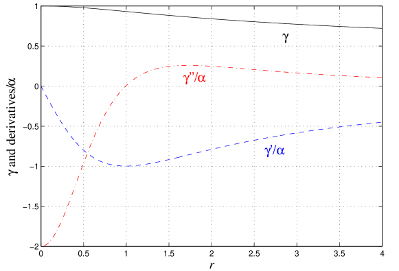
Fig. 3: Plot of $\gamma$ [eq. (11)], $\gamma^{\prime}/\alpha$ [eq. (12)], and $\gamma^{\prime\prime}/\alpha$ [eq. (13)] versus $r$ for $\alpha=0.1$. All three functions go to zero for $r\to\infty$, with no extrema other than those shown.

What remains is, in principle, merely a matter of algebra to verify that this trial function, for sufficiently small $\alpha$, satisfies the variational condition (9). In practice, some care is required in appropriately bounding each of the integrals and in taking the limits in the proper order, and we review this process below.

We substitute the trial function (10) for $\mathbf{H}$ into the left-hand side of eq. (9):

$$\begin{split}&\varepsilon_{c}\int\frac{1}{\varepsilon({\mathbf{r}})}\left\|\left(\nabla+i\beta\hat{z}\right)\times\mathbf{H}(r,\phi)\right\|^{2}d^{2}\mathbf{r}-\beta^{2}\int\|\mathbf{H}\|^{2}d^{2}\mathbf{r}\\ &=\varepsilon_{c}\int\left(\frac{1}{\varepsilon_{c}}+\Delta(\mathbf{r})\right)\left\|\hat{z}\frac{1}{r}\left[\frac{\partial}{\partial r}(rH_{\phi})-\frac{\partial H_{r}}{\partial\phi}\right]+i\beta\hat{z}\times{\mathbf{H}}\right\|^{2}d^{2}\mathbf{r}-\beta^{2}\int{\|\mathbf{H}\|^{2}}d^{2}\mathbf{r}\\ &=\varepsilon_{c}\int\left(\frac{1}{\varepsilon_{c}}+\Delta(\mathbf{r})\right)\left(\frac{\sin^{2}\phi}{r^{2}}\left\{\left[r(r\gamma)^{\prime}\right]^{\prime}-\gamma\right\}^{2}+\beta^{2}\|\mathbf{H}\|^{2}\right)d^{2}\mathbf{r}-\beta^{2}\int{\|\mathbf{H}\|^{2}}d^{2}\mathbf{r}\\ &=\varepsilon_{c}\int\left(\frac{1}{\varepsilon_{c}}+\Delta(\mathbf{r})\right)\frac{\sin^{2}\phi}{r^{2}}\left(3r\gamma^{\prime}+r^{2}\gamma^{\prime\prime}\right)^{2}d^{2}\mathbf{r}+\varepsilon_{c}\int\beta^{2}\Delta(\mathbf{r})\|\mathbf{H}\|^{2}d^{2}\mathbf{r}\\ \end{split}$$ (14)

We proceed to show that the last line of the above expression is negative in the limit $\alpha\to 0$, thus satisfying the condition for the existence of bound modes. We first examine the second term of eq. (14):

$$\lim_{\alpha\to{0}}\int\beta^{2}\Delta(\mathbf{r})\|\mathbf{H}\|^{2}d^{2}\mathbf{r}=\beta^{2}\int\Delta(\mathbf{r})d^{2}\mathbf{r}<0.$$ (15)

The key fact here is that we are able to interchange the $\alpha\to 0$ limit and the integral in this case, thanks to Lebesgue’s Dominated Convergence Theorem (LDCT) [33]: whenever the absolute value of the integrand is bounded above (for sufficiently small $\alpha$) by an $\alpha$-independent function with a finite integral, LDCT guarantees that the $\alpha\to 0$ limit can be interchanged with the integral. In particular, the absolute value of this integrand is bounded above by $|\Delta|$ multiplied by some constant (since $|\mathbf{H}|$ is bounded by a constant: $|\gamma|\leq 1$ and $|r\gamma^{\prime}|$ is also easily seen to be bounded above for sufficiently small $\alpha$), and $|\Delta|$ has a finite integral by assumption. Since $\lim_{\alpha\to 0}|\mathbf{H}|^{2}=1$, we obtain eq. (4), which is negative by assumption.

Now we must show that the remaining first term of eq. (14) goes to zero as $\alpha\to 0$, completing our proof. This term is proportional to $(\varepsilon_{c}^{-1}+\Delta)$, but the $\Delta$ terms trivially go to zero by the same arguments as above: $\Delta$ allows the limit to be interchanged with the integration by LDCT, and as $\alpha\to 0$ the $\gamma^{\prime}$ and $\gamma^{\prime\prime}$ terms go to zero. The remaining $\varepsilon_{c}^{-1}$ terms can be bounded above by a sequence of inequalities as follows:

$$\begin{split}&\lim_{\alpha\to 0}\int_{0}^{\infty}\int_{0}^{2\pi}\frac{\sin^{2}\phi}{r^{2}}(3r\gamma^{\prime}+r^{2}\gamma^{\prime\prime})^{2}r\,dr\,d\phi\\ &=16\pi\lim_{\alpha\to 0}\int_{0}^{\infty}\alpha^{2}r^{3}(r^{2}+1)^{2\alpha-2}\gamma^{2}\left[-2+\alpha r^{2}(r^{2}+1)^{\alpha-1}+(1-\alpha)r^{2}(r^{2}+1)^{-1}\right]^{2}dr\\ &\leq 16\pi\lim_{\alpha\to 0}\int_{0}^{\infty}\alpha^{2}r(r^{2}+1)^{2\alpha-1}\gamma^{2}\left[2+\alpha(r^{2}+1)^{\alpha}+(1-\alpha)\right]^{2}dr\\ &=16\pi\lim_{\alpha\to 0}\int_{1}^{\infty}\alpha^{2}t^{4\alpha-1}e^{2-2t^{2\alpha}}\left[(3-\alpha)+\alpha t^{2\alpha}\right]^{2}dt\\ &\leq 8\pi\lim_{\alpha\to 0}\int_{0}^{\infty}\alpha u\,e^{2-2u}\left[(3-\alpha)+\alpha u\right]^{2}du\\ &=8\pi e^{2}\lim_{\alpha\to 0}\alpha\left[\frac{3}{8}\alpha^{2}+\frac{1}{2}\alpha(3-\alpha)+\frac{1}{4}\left(3-\alpha\right)^{2}\right]=0.\end{split}$$ (16)

From the first to second line, we substituted eqs. (12) and (13) and simplified. From the second to third line, we bounded the integrand above by flipping negative terms into positive ones and replacing $r^{2}$ with $r^{2}+1$. From the third to the fourth line, we made a change of variables $t^{2}=r^{2}+1$. Then, from the fourth to fifth line, we made another change of variable $u=t^{2\alpha}$, and bounded the integral above by changing the lower limit from $u=1$ to $u=0$. The final integral can be performed exactly and goes to zero, completing the proof.

4 General periodic claddings

In the previous section we considered $z$-invariant waveguides with a homogeneous cladding and isotropic materials (for example, conventional optical fibers). We now generalize the proof in three ways, by allowing:

• transverse periodicity in the cladding material (photonic-crystal fibers),

• a core and cladding that are periodic in $z$ with period $a$ ($a\to 0$ for the $z$-invariant case),

• anisotropic $\varepsilon_{c}$ and $\Delta\varepsilon$ materials ($\varepsilon$ is a $3\times 3$ positive-definite Hermitian matrix).

In particular, we consider dielectric functions of the form:

$$\varepsilon(x,y,z)=\varepsilon_{c}(x,y,z)+\Delta\varepsilon(x,y,z),$$ (17)

where the cladding dielectric tensor $\varepsilon_{c}(x,y,z)=\varepsilon_{c}(x,y,z+a)$ is $z$-periodic and also periodic in the $xy$ plane (with an arbitrary unit cell and lattice), and the core dielectric tensor change $\Delta\varepsilon(x,y,z)=\Delta\varepsilon(x,y,z+a)$ is $z$-periodic with the same period $a$. Both $\varepsilon_{c}$ and the total $\varepsilon$ must be positive-definite Hermitian tensors. As defined in eq. (3), we denote by $\Delta$ the change in the inverse dielectric tensor. Similar to the isotropic case, we require that $\int|\Delta_{ij}|$ be finite for integration over the $xy$ plane and one period of $z$, for every tensor component $\Delta_{ij}$. We also require that the components of $\varepsilon_{c}^{-1}$ be bounded above.

In the homogeneous-cladding case, any light mode that lies beneath the (linear) light line of the cladding is guided. We have shown that such a mode always exists, for all $\beta$, under the condition of eq. (4), by showing that the variational upper bound on its frequency lies below the light line. In the case of a periodic cladding, the light line is the dispersion relation of the fundamental space-filling mode of the cladding, which corresponds to the lowest-frequency mode at each given propagation constant $\beta$ [2, 3, 4, 5]. This light “line” is, in general, no longer straight, and there are mechanisms for guidance that are not available in the previous case, such as bandgap guidance [2, 3, 4, 5]. Bandgap-guided modes may exist above the light line and are, in general, not cutoff-free because the gap has a finite bandwidth. Here, we only consider index-guided modes, which are guided because they lie below the light line. We will follow the same general procedure as in the previous section to derive the sufficient condition [eq. (1)] to guarantee the existence of guided modes. The homogeneous-cladding case is then a special case of this more general theorem, recovering eq. (4) (but generalizing it to $z$-periodic cores), where in that case the cladding fundamental mode $\mathbf{D}_{c}$ is a constant and can be pulled out of the integral. The case of a $z$-homogeneous fiber is just the special case $a\to 0$, eliminating the $z$ integral in eq. (1).

The proof is similar in spirit to that of the homogeneous-cladding case. At each $\beta$, the eigenmodes $\mathbf{H}(x,y,z)e^{i\beta z-i\omega t}$ satisfy the same Hermitian eigenproblem (5) and transversality constraint (7) as before. We have a similar variational theorem to eq. (8) [5], except that, in the case of $z$-periodicity, we now integrate over one period in $z$ as well as over $x$ and $y$.

$$\frac{\omega_{\mathrm{min}}^{2}(\beta)}{c^{2}}=\inf_{\nabla_{\beta}\cdot\mathbf{H}=0}\frac{\int\mathbf{H}^{*}\cdot\hat{\Theta}_{\beta}\mathbf{H}}{\int\mathbf{H}^{*}\cdot\mathbf{H}}.$$ (18)

As before, to prove the existence of a guided mode we will find a trial function $\mathbf{H}$ such that this upper bound, called the “Rayleigh quotient” for $\mathbf{H}$, is below the light line $\omega_{c}(\beta)^{2}/c^{2}$. The corresponding condition on $\mathbf{H}$ can be written [similar to eq. (9)]:

$$\int\mathbf{H}^{*}\cdot\hat{\Theta}_{\beta}\mathbf{H}-\frac{\omega_{c}^{2}(\beta)}{c^{2}}\int\mathbf{H}^{*}\cdot\mathbf{H}<0.$$ (19)

We considered a variety of trial functions, inspired by the Yang and de Llano quantum case [11], before finding the following choice that allows us to prove the condition (19). Similar to eq. (10), we want a slowly decaying function proportional to $\gamma(r)=e^{1-(r^{2}+1)^{\alpha}}$, from eq. (11), that in the $\alpha\to 0$ (weak guidance) limit approaches the cladding fundamental mode $\mathbf{H}_{c}$. As before, the trial function must be transverse ($\nabla_{\beta}\cdot\mathbf{H}=0$), which motivated us to write the trial function in terms of the corresponding vector potential. We denote by $\mathbf{A}_{c}$ the vector potential corresponding to the cladding fundamental mode $\mathbf{H}_{c}=\nabla_{\beta}\times\mathbf{A}_{c}$. In terms of $\mathbf{A}_{c}$ and $\gamma$, our trial function is then:

$$\mathbf{H}=\nabla_{\beta}\times\left(\gamma\mathbf{A}_{c}\right)=\gamma\mathbf{H}_{c}+\nabla\gamma\times\mathbf{A}_{c}.$$ (20)

For convenience, we choose $\mathbf{A}_{c}$ to be Bloch-periodic (like $\mathbf{H}_{c}$, since $\mathbf{A}_{c}$ also satisifies a periodic Hermitian generalized eigenproblem and hence Bloch’s theorem applies). In contrast, our previous homogeneous-cladding trial function [eq. (10)] corresponds to a different gauge choice with an unbounded vector potential $\mathbf{A}_{c}=-\frac{1}{i\beta}\hat{\mathbf{y}}+\nabla_{\beta}\psi$, differing from a constant vector potential via the gauge function $\psi=\frac{r}{i\beta}\sin\phi+e^{-i\beta z}$.

Substituting eq. (20) into the left hand side of our new guidance condition (19), we obtain five categories of terms to analyze:

1. terms that contain $\Delta=\varepsilon^{-1}-\varepsilon_{c}^{-1}$,

2. terms that cancel due to the eigenequation (5),

3. terms that have one first derivative of $\gamma$,

4. terms that have $(\gamma^{\prime})^{2}$,

5. terms that have $\gamma^{\prime}\gamma^{\prime\prime}$ or $(\gamma^{\prime\prime})^{2}$.

Category (i) will give us our condition for guided modes, eq. (1), while category (ii) will be cancelled exactly in eq. (19). We show in the appendix that all of the terms in category (iii) exactly cancel one another. The terms in categories (iv) and (v) all vanish in the $\alpha\to 0$ limit; we distinguish them because category (v) turns out to be easier to analyze. There are no terms with $\gamma^{\prime\prime}$ alone, as these can be integrated by parts to obtain category (iii) and (iv) terms. In the appendix, we provide an exhaustive listing of all the terms and how they combine as described above. In this section, we only outline the basic structure of this algebraic process, and explain why the category (iv) and (v) terms vanish as $\alpha\to 0$.

Category (i) consists only of one term:

$$\begin{split}&\lim_{\alpha\rightarrow 0}\int\mathbf{H}^{*}\cdot\left(\nabla_{\beta}\times\Delta\nabla_{\beta}\times\mathbf{H}\right)\\ =&\int\mathbf{H}_{c}^{*}\cdot\left(\nabla_{\beta}\times\Delta\nabla_{\beta}\times\mathbf{H}_{c}\right)\\ =&\int\left(\nabla_{\beta}\times\mathbf{H}_{c}\right)^{*}\cdot\Delta\left(\nabla_{\beta}\times\mathbf{H}_{c}\right)\\ =&\frac{\omega_{c}^{2}}{c^{2}}\int\mathbf{D}_{c}^{*}\cdot\Delta\mathbf{D}_{c}\\ \end{split}$$ (21)

From the first to the second line, we interchanged the limit with the integration, thanks to the LDCT condition as in Sec. 3, since the magnitudes of all of the terms in the integrand are bounded above by the tensor components $|\Delta_{ij}|$ multiplied by some $\alpha$-independent constants, and $|\Delta_{ij}|$ has a finite integral by assumption. (In particular, the $\mathbf{A}_{c}$ fundamental mode and its curls are bounded functions, being Bloch-periodic, and $\gamma$ and its first two derivatives are bounded for sufficiently small $\alpha$.) The result is precisely the left-hand side of eq. (1), which is negative by assumption.

Next, we would like to cancel $-\frac{\omega_{c}^{2}}{c^{2}}\int\mathbf{H}^{*}\cdot\mathbf{H}$ by the eigen-equation (5). Thus, we examine the term $\int\mathbf{H}^{*}\cdot\left(\nabla_{\beta}\times\varepsilon_{c}^{-1}\gamma\nabla_{\beta}\times{\mathbf{H}_{c}}\right)$ (which comes from the term where the right-most curl falls on $\mathbf{H}_{c}$ rather than $\gamma$) below:

$$\begin{split}&\int\mathbf{H}^{*}\cdot\left(\nabla_{\beta}\times\varepsilon_{c}^{-1}\gamma\nabla_{\beta}\times{\mathbf{H}_{c}}\right)\\ =&\int\mathbf{H}^{*}\cdot\left(\gamma\nabla_{\beta}\times\varepsilon_{c}^{-1}\nabla_{\beta}\times\mathbf{H}_{c}+\left(\nabla\gamma\right)\times\varepsilon_{c}^{-1}\nabla_{\beta}\times\mathbf{H}_{c}\right)\\ =&\int\mathbf{H}^{*}\cdot\gamma\frac{\omega_{c}^{2}}{c^{2}}\mathbf{H}_{c}+\int\mathbf{H}^{*}\cdot\left(\nabla\gamma\times\varepsilon_{c}^{-1}\nabla_{\beta}\times\mathbf{H}_{c}\right)\\ =&\int\mathbf{H}^{*}\cdot\frac{\omega_{c}^{2}}{c^{2}}\mathbf{H}-\int\mathbf{H}^{*}\cdot\frac{\omega_{c}^{2}}{c^{2}}\nabla\gamma\times\mathbf{A}_{c}+\int\mathbf{H}^{*}\cdot\left(\nabla\gamma\times\varepsilon_{c}^{-1}\nabla_{\beta}\times\mathbf{H}_{c}\right)\\ \end{split}$$ (22)

From the second to the third lines, we used the eigenequation (5), and from the third to the fourth lines we used the definition (20) of $\mathbf{H}$ in terms of $\mathbf{H}_{c}$. The first term of the last line above cancels $-\frac{\omega_{c}^{2}}{c^{2}}\int\mathbf{H}^{*}\cdot\mathbf{H}$ in eq. (19). The second and third terms contain two category (iii) terms: $\frac{\omega_{c}^{2}}{c^{2}}\int\gamma\mathbf{H}_{c}\cdot\left(\nabla\gamma\times\mathbf{A}_{c}\right)$ and $i\omega_{c}\int\gamma\nabla\gamma\cdot\mathbf{E}_{c}\times\mathbf{H}_{c}^{*}$, both of which will be exactly cancelled as described in the appendix, as well as some category (iv) and (v) terms.

The category (iv) integrands are all of the form $(\gamma^{\prime})^{2}$ multiplied by some bounded function (a product of the various Bloch-periodic fields as well as the bounded $\varepsilon_{c}^{-1}$). This integrand can then be bounded above by replacing the bounded function with the supremum $B$ of its magnitude, at which point the integral is bounded above by $2\pi B\int_{0}^{\infty}(\gamma^{\prime})^{2}r\,dr$. However, such integrands were among the terms we already analyzed in the homogeneous-cladding case, in eq. (16), and we explicitly showed that such integrals go to zero as $\alpha\to 0$.

The category (v) integrands could also be explicitly shown to vanish as $\alpha\to 0$, similar to eq. (16), but a simpler proof of the same fact can be constructed via the LDCT condition. In particular, similar to the previous paragraph, after replacing bounded functions with their suprema we are left with cylindrical-coordinate integrands of the form $\gamma^{\prime}\gamma^{\prime\prime}r$ and $(\gamma^{\prime\prime})^{2}r$. Both of these integrands, however, are bounded above by an $\alpha$-independent function with a finite integral, and hence LDCT allows us to put the $\alpha\to 0$ limit inside the integral and set the integrands to zero. Specifically, by inspection of eqs. (12) and (13), $|\gamma^{\prime}\gamma^{\prime\prime}|r<4r^{2}(1+2+2)/(r^{2}+1)^{2-\delta}$ and $(\gamma^{\prime\prime})^{2}r<4r(1+2+2)^{2}/(r^{2}+1)^{2-\delta}$ for $\alpha<\delta/4$, and both of these upper bounds have finite integrals, if we take $\delta$ to be some number $<1/2$, since they decay faster than $1/r$.

In summary, we have shown that, if eq. (1) is satisfied, then the variational upper bound for our trial function [eq. (20)] is below the light line, and therefore an index-guided mode is guaranteed to exist. The special cases of this theorem, as discussed in the introduction, immediately follow.

5 Substrates, dispersive materials, and finite-size effects

In this section, we briefly discuss several situations that lie outside of the underlying assumptions of our theorem: waveguides sitting on substrates, dispersive ($\omega$-dependent) materials, and finite-size claddings.

An optical fiber is completely surrounded by a single cladding material, but the situation is quite different in integrated optical waveguides. There, it is common to have an asymmetrical cladding, with air above the waveguide and a low-index material (e.g. oxide) below the waveguide, such as in strip or ridge waveguides [12, 13, 14]. In such cases, it is well known that the fundamental guided mode has a low-frequency cutoff even when the waveguide consists of strictly nonnegative $\Delta\varepsilon$ [12, 14]. This does not contradict our theorem because we required the cladding to be periodic in both transverse directions, whereas a substrate is not periodic in the vertical direction.

We have also assumed non-dispersive materials in our proof. What happens when we have more realistic, dispersive materials? Suppose that $\varepsilon$ depends on $\omega$ but has negligible absorption (so that guided modes are still well-defined). For a given $\omega$, we can construct a frequency-independent $\varepsilon$ structure matching the actual $\varepsilon$ at that $\omega$, and apply our theorem to determine whether there are guided modes at $\omega$. The simplest case is when $\Delta\varepsilon\geq 0$ for all $\omega$, in which case we must still obtain cutoff-free guided modes. The theorem becomes more subtle to apply when $\Delta\varepsilon<0$ in some regions, because not only must one perform the integral of eq. (1) to determine the existence of guided modes, but the condition (1) is for a fixed $\beta$ while the integrand is for a given frequency, and the frequency of the guided mode is unknown a priori.

Finally, any real structure has a finite cladding. Both numerically and experimentally, this makes it difficult to study the long-wavelength regime because the modal diameter increases rapidly with wavelength (i.e. the frequency approaches the light line and the transverse decay rate becomes very slow)—in fact, it seems likely that the modal diameter will increase exponentially with the wavelength. In quantum mechanics (scalar waves) with a potential well of depth $V$, the decay length of the bound mode increases as $e^{C/V}$ when $V\to 0$, for some constant $C$ [27, 11]. In electromagnetism, for the long wavelength limit, a homogenized effective-medium $\tilde{\varepsilon}$ description of the structure becomes applicable [25], and in this effective near-homogeneous limit the modes are described by a scalar wave equation with a “potential” $-\omega^{2}\Delta\tilde{\varepsilon}$ [34], and hence the quantum analysis should apply. Thus, by this informal argument, we would expect the modal diameter to expand proportional to $e^{C\lambda^{2}}$ for some constant $C$ (where $\lambda=2\pi c/\omega$ is the vacuum wavelength), but a more explicit proof would be desirable.

6 Concluding remarks

We have demonstrated sufficient conditions for the existence of cutoff-free guided modes for general microstructured dielectric fibers, periodic in either or both the $z$ direction and in the transverse plane. The results are a generalization of previous results on the existence of such modes in fibers with a homogeneous cladding index. Our theorem allows one to understand the guidance in many very complicated structures analytically, and enables one to rigorously guarantee guided modes in many structures (especially those where $\Delta\varepsilon\geq 0$ everywhere) by inspection. There remain a number of interesting questions for future study, however, some of which we outline below.

Our eq. (1) is a sufficient condition for index-guided modes, but it is certainly not necessary in general: even when it is violated, one can have guided modes with a cutoff (as for W-profile fibers [17] or waveguides on substrates [12, 14]), or other types of guided modes (such as bandgap-guided modes [2, 3, 4, 5]). However, these other types of guides modes in dielectric waveguides have a long-wavelength cutoff, so one can pose the question: is eq. (1) a necessary condition for cutoff-free guided modes (where $\mathbf{D}_{c}$ is given by the long-wavelength limit of the cladding fundamental mode) in dielectric waveguides (as opposed to TEM modes in metallic coaxial waveguides, which also have no cutoff [35])? Based on theoretical reasoning and some numerical evidence, we suspect that the answer is no, but that it may be possible to modify eq. (1) to obtain a necessary condition. In particular, the variational theorem is closely related to first-order perturbation theory: if one has a small perturbation $\Delta\varepsilon$ and substitutes the unperturbed field into the Rayleigh quotient, the result is the first-order perturbation in the eigenvalue. However, when $\Delta\varepsilon$ is large, even if the volume of the perturbation is small, perturbation theory requires a correction due to the electric-field discontinuity at the interface [36]. In the long-wavelength limit, perturbation theory is corrected by computing the quasi-static polarizability of the perturbation [36], and we conjecture that a similar correction to our trial field may allow one to derive a necessary condition for the absence of a cutoff. Equation (1) is still a sufficient condition (the variational theorem still holds even with a suboptimal trial function), but the preceding considerations predict that it will become farther from a necessary condition for the absence of a cutoff as $\Delta\varepsilon$ is increased, and this prediction seems to be confirmed by preliminary numerical experiments with W-profile fibers.

Let us also mention five other interesting directions to pursue. First, Ref. 9 actually proved a somewhat stronger condition than eq. (1) for homogeneous claddings, in that they showed the existence of guided modes when the integral was $\leq 0$ (and $\Delta\varepsilon>0$ in some region) rather than $<0$ as in our condition. Although the $=0$ case seems unlikely to be experimentally or numerically significant, we suspect that a similar generalization should be possible for our theorem (re-weighting the integrand to make it negative and then taking a limit as in Ref. 9). Second, as discussed in Sec. 5, it would be desirable to develop a sufficient condition at a fixed $\omega$ rather than at a fixed $\beta$, although we are not sure whether this is possible. Third, one would like a more explicit confirmation of the argument, in Sec. 5, that the modal diameter should asymptotically increase exponentially with the square of the wavelength. Fourth, it might be interesting to consider the case of “Bragg fiber” geometries consisting of “periodic” sequences of concentric layers [37], which are not strictly periodic because the layer curvature decreases with radius. Finally, as we mentioned in Sec. 2, it is possible to extend the theorem to a condition for two guided modes in many cases where the cladding fundamental mode is doubly degenerate, and we are currently preparing another manuscript describing this result along with conditions for truly single-mode (“single-polarization”) waveguides.

Appendix: All Rayleigh-quotient terms

In this appendix, we provide an exhaustive listing of all the terms that appear when the trial function [eq. (20)] is substituted into eq. (19) (the condition to be satisfied, a rearrangement of the Rayleigh quotient bound). Since the terms that contain $\Delta$ [category (i)] were already fully analyzed in Sec. 4 (since for these terms the limits could be trivially interchanged), we consider only the remaining terms involving $\varepsilon_{c}(\mathbf{r})$. More specifically, the only non-trivial term to analyze is the $\Delta$-free part of the left-most integral in eq. (19):

$$\begin{split}&\int\mathbf{H}^{*}\cdot\left(\nabla_{\beta}\times\varepsilon_{c}^{-1}\nabla_{\beta}\times\mathbf{H}\right)\\ &=\int\mathbf{H}^{*}\cdot\left(\nabla_{\beta}\times\varepsilon_{c}^{-1}\gamma\nabla_{\beta}\times{\mathbf{H}_{c}}\right)+\int\mathbf{H}^{*}\cdot\left(\nabla_{\beta}\times\varepsilon_{c}^{-1}\nabla\gamma\times{\mathbf{H}_{c}}\right)\\ &\quad{}+\int\mathbf{H}^{*}\cdot\left(\nabla_{\beta}\times\varepsilon_{c}^{-1}\nabla_{\beta}\times\left(\nabla\gamma\times{\mathbf{A}_{c}}\right)\right).\end{split}$$ (23)

We have already seen, in eq. (22), that the first term breaks down into a term that cancels $\frac{\omega_{c}^{2}}{c^{2}}\int\mathbf{H}^{*}\cdot\mathbf{H}$ in eq. (19), via the eigen-equation, and two other terms. Removing the terms cancelled by the eigenequation, and substituting $-i\frac{\omega_{c}}{c}\mathbf{E}_{c}$ for $\varepsilon_{c}^{-1}\nabla_{\beta}\times\mathbf{H}_{c}$ (Ampère’s law), we have:

$$\begin{split}&\quad{}-\frac{\omega_{c}^{2}}{c^{2}}\int\mathbf{H}^{*}\cdot\left(\nabla\gamma\times\mathbf{A}_{c}\right)+\int\mathbf{H}^{*}\cdot\left[\nabla\gamma\times\left(-i\frac{\omega_{c}}{c}\mathbf{E}_{c}\right)\right]\\ &\quad{}+\int\mathbf{H}^{*}\cdot\nabla_{\beta}\times\varepsilon_{c}^{-1}\left[\nabla\gamma\times\mathbf{H}_{c}+\nabla_{\beta}\times\left(\nabla\gamma\times\mathbf{A}_{c}\right)\right]\\ &=-\frac{\omega_{c}^{2}}{c^{2}}\int\left[\gamma\mathbf{H}_{c}+\nabla\gamma\times\mathbf{A}_{c}\right]^{*}\cdot\left(\nabla\gamma\times\mathbf{A}_{c}\right)-i\frac{\omega_{c}}{c}\int\gamma\nabla\gamma\cdot\left(\mathbf{E}_{c}\times\mathbf{H}_{c}^{*}\right)\\ &\quad{}-i\frac{\omega_{c}}{c}\int\left(\nabla\gamma\times\mathbf{A}_{c}\right)^{*}\cdot\left(\nabla\gamma\times\mathbf{E}_{c}\right)+\int\left(\gamma\nabla_{\beta}\times\mathbf{H}_{c}\right)^{*}\cdot\varepsilon_{c}^{-1}\left[\nabla\gamma\times\mathbf{H}_{c}+\nabla_{\beta}\times\left(\nabla\gamma\times\mathbf{A}_{c}\right)\right]\\ &\quad{}+\int\left(\nabla\gamma\times\mathbf{H}_{c}\right)^{*}\cdot\varepsilon_{c}^{-1}\left[\nabla\gamma\times\mathbf{H}_{c}+\nabla_{\beta}\times\left(\nabla\gamma\times\mathbf{A}_{c}\right)\right]\\ &\quad{}+\int\left(\nabla_{\beta}\times\nabla\gamma\times\mathbf{A}_{c}\right)^{*}\cdot\varepsilon_{c}^{-1}\left[\nabla\gamma\times\mathbf{H}_{c}+\nabla_{\beta}\times\left(\nabla\gamma\times\mathbf{A}_{c}\right)\right]\\ &=-\frac{\omega_{c}^{2}}{c^{2}}\int\gamma\mathbf{H}_{c}^{*}\cdot\left(\nabla\gamma\times\mathbf{A}_{c}\right)-\frac{\omega_{c}^{2}}{c^{2}}\int\left\|\nabla\gamma\times\mathbf{A}_{c}\right\|^{2}-i\frac{\omega_{c}}{c}\int\gamma\nabla\gamma\cdot\left(\mathbf{E}_{c}\times\mathbf{H}_{c}^{*}\right)\\ &\quad{}-i\frac{\omega_{c}}{c}\int\left(\nabla\gamma\times\mathbf{A}_{c}\right)^{*}\cdot\left(\nabla\gamma\times\mathbf{E}_{c}\right)+i\frac{\omega_{c}}{c}\int\gamma\mathbf{E}_{c}^{*}\cdot\left(\nabla\gamma\times\mathbf{H}_{c}\right)\\ &\quad{}+i\frac{\omega_{c}}{c}\int\gamma\left(\nabla_{\beta}\times\mathbf{E}_{c}\right)^{*}\cdot\left(\nabla\gamma\times\mathbf{A}_{c}\right)+i\frac{\omega_{c}}{c}\int\left(\nabla\gamma\times\mathbf{E}_{c}\right)^{*}\cdot\left(\nabla\gamma\times\mathbf{A}_{c}\right)\\ &\quad{}+\int\left(\nabla\gamma\times\mathbf{H}_{c}\right)^{*}\cdot\varepsilon_{c}^{-1}\left(\nabla\gamma\times\mathbf{H}_{c}\right)\\ &\quad{}+\left(\int\left(\nabla\gamma\times\mathbf{H}_{c}\right)^{*}\cdot\varepsilon_{c}^{-1}\left[\nabla_{\beta}\times\left(\nabla\gamma\times\mathbf{A}_{c}\right)\right]+\mathrm{c.c.}\right)\\ &\quad{}+\int\left(\nabla_{\beta}\times\left(\nabla\gamma\times\mathbf{A}_{c}\right)\right)^{*}\cdot\varepsilon_{c}^{-1}\left(\nabla_{\beta}\times\left(\nabla\gamma\times\mathbf{A}_{c}\right)\right).\end{split}$$ (24)

Above, the first “$=$” step is obtained by substituting the trial function for $\mathbf{H}$, integrating some of the $\nabla_{\beta}\times{}$ operators by parts, and distributing the derivatives of $\gamma\mathbf{H}_{c}$ by the product rule. The second step is obtained by using Ampère’s law again, combined with integrations by parts and the product rule; “c.c.” stands for the complex conjugate of the preceding expression. Continuing, we obtain:

$$\begin{split}&=-\frac{\omega_{c}^{2}}{c^{2}}\int\gamma\mathbf{H}_{c}^{*}\cdot\left(\nabla\gamma\times\mathbf{A}_{c}\right)-\frac{\omega_{c}^{2}}{c^{2}}\int\left\|\nabla\gamma\times\mathbf{A}_{c}\right\|^{2}-2i\frac{\omega_{c}}{c}\int\gamma\nabla\gamma\cdot\Re\left\{\mathbf{E}_{c}\times\mathbf{H}_{c}^{*}\right\}\\ &\quad{}+\left(i\frac{\omega_{c}}{c}\int\left(\nabla\gamma\times\mathbf{A}_{c}\right)\cdot\left(\nabla\gamma\times\mathbf{E}_{c}\right)^{*}+\mathrm{c.c.}\right)+\frac{\omega_{c}^{2}}{c^{2}}\int\gamma\mathbf{H}_{c}^{*}\cdot\left(\nabla\gamma\times\mathbf{A}_{c}\right)\\ &\quad{}+\int\left(\nabla\gamma\times\mathbf{H}_{c}\right)^{*}\cdot\varepsilon_{c}^{-1}\left(\nabla\gamma\times\mathbf{H}_{c}\right)+\left(\int\left(\nabla\gamma\times\mathbf{H}_{c}\right)^{*}\cdot\varepsilon_{c}^{-1}\left[\nabla_{\beta}\times\left(\nabla\gamma\times\mathbf{A}_{c}\right)\right]+\mathrm{c.c.}\right)\\ &\quad{}+\int\left(\nabla_{\beta}\times\left(\nabla\gamma\times\mathbf{A}_{c}\right)\right)^{*}\cdot\varepsilon_{c}^{-1}\left(\nabla_{\beta}\times\left(\nabla\gamma\times\mathbf{A}_{c}\right)\right)\\ \end{split}$$ (25)

In obtaining this expression, we have grouped terms into complex-conjugate pairs and used Faraday’s law to replace $\nabla_{\beta}\times\mathbf{E}_{c}$ with $i\frac{\omega_{c}}{c}\mathbf{H}_{c}$. At this point, we have two $\frac{\omega_{c}^{2}}{c^{2}}\int\gamma\mathbf{H}_{c}^{*}\cdot\left(\nabla\gamma\times\mathbf{A}_{c}\right)$ terms that exactly cancel. All of the remaining terms, except for $-i\frac{\omega_{c}}{c}\int\gamma\nabla\gamma\cdot\Re\left\{\mathbf{E}_{c}\times\mathbf{H}_{c}^{*}\right\}$, are multiples of two first or higher derivatives of $\gamma$, corresponding to category (iv) and (v) terms, which we proved to vanish in Sec. 4.

The only remaining term is the $\mathbf{E}_{c}\times\mathbf{H}_{c}^{*}$ term, in category (iii). This term is identically zero (for any $\alpha\geq 0$) because it is purely imaginary, whereas all of the other terms are purely real and the overall expression must be real. More explicitly:

$$\begin{split}&-2i\frac{\omega_{c}}{c}\int\gamma\nabla\gamma\cdot\Re\left\{\mathbf{E}_{c}\times\mathbf{H}_{c}^{*}\right\}\\ &\quad=-2i\frac{\omega_{c}}{2c}\int\nabla\gamma^{2}\cdot\Re\left\{\mathbf{E}_{c}\times\mathbf{H}_{c}^{*}\right\}\\ &\quad=-i\frac{\omega_{c}}{c}\int\nabla\cdot\left(\gamma^{2}\Re\left\{\mathbf{E}_{c}\times\mathbf{H}_{c}^{*}\right\}\right)+i\frac{\omega_{c}}{c}\int\gamma^{2}\nabla\cdot\left(\Re\left\{\mathbf{E}_{c}\times\mathbf{H}_{c}^{*}\right\}\right)\\ \end{split}$$ (26)

The first term of the last line is zero by the divergence theorem (transforming it into a surface integral at infinity), since $\gamma\to 0$ at infinity. For the second term, the integrand is the divergence of the time-average Poynting vector $\Re\left\{\mathbf{E}_{c}\times\mathbf{H}_{c}^{*}\right\}$, which equals the time-average rate of change of the energy density [34], which is identically zero for any lossless eigenmode (such as the cladding fundamental mode).