Should particle trajectories comply with the transverse momentum distribution?

Abstract

The momentum distributions associated with both the wave function of a particle behind a grating and the corresponding Bohmian trajectories are investigated and compared. Near the grating, it is observed that the former does not depend on the distance from the grating, while the latter changes with this distance. However, as one moves further apart from the grating, in the far field, both distributions become identical.

1 Introduction

Quantum interference experiments where beams of one particle at a time are used have intensified the theoretical investigation of the topology of particle trajectories behind the interference grating ref1 ; ref2 ; ref3 ; ref4 ; ref5 ; ref6 ; ref7 ; ref8 . The aim of all the approaches developed in this direction is to get consistency between the quantum mechanical particle distribution and the distribution associated with the trajectories of the particles. In this paper we compare the features of Bohmian trajectories with those displayed by the trajectories determined using the momentum distribution (MD trajectories) associated with the wave function of the particle. As is well known, Bohmian trajectories follow the flux lines of the quantum flow, and therefore reproduce exactly the quantum mechanical distribution in both the far and near field ref1 ; ref2 ; ref3 ; ref4 ; ref6 ; ref8 . In particular, it is remarkable the consistency of a set of Bohmian trajectories in the near field behind a multiple slit grating within the context of the Talbot effect ref8 . This effect has been observed experimentally with relatively heavy particles, such as Na atoms ref8-a or Bose-Einstein condensates ref8-b .

Moreover, here we also study the momentum distribution associated with Bohmian trajectories, and compare it with the momentum distribution associated with the wave function of the particle. We find that in the far field these two distributions are identical. However, in the near field, the distribution of transverse momenta associated with the Bohmian trajectories changes with the distance from the grating, and therefore differs from the momentum distribution associated with the wave function.

The essential feature of the Bohmian deterministic trajectories is that a particle passing through different slits will never reach the same point on the detection screen ref4 . On the contrary, this limitation does not hold for MD trajectories arising from different slits, which may reach the same point on the screen ref5 ; ref7 . The momenta of particles moving along MD trajectories are distributed according to the momentum distribution determined by the wave function of the particle. The probability of arrival of a particle to a given point on the screen depends on: (1) the slit through which it passed and (2) the presence of other slits. The second type of dependence is a consequence of the dependence of this probability on the transverse momentum distribution, which depends on the properties of the grating as a whole ref5 . As shown, MD trajectories reproduce fairly well the quantum mechanical space distribution in the far field.

2 Wave function of a particle behind a grating

The motion of a particle behind a grating is determined by its wave function. Here, we assume that in front of the grating ($y<0$) we have a plane wave with initial momentum $\vec{p}=\hbar\vec{k}=\hbar k\vec{i}_{y}$ (and de Broglie wavelength $\lambda=2\pi/k$), moving along the longitudinal direction $y$. Behind the grating ($y\geq 0$), the solution can be expressed as a product of the longitudinal part, a plane wave, and the transverse part, i.e.,

$$\Psi(x,y,t)=Be^{iky}e^{-i\omega t}\psi(x,t),$$ (1)

where $B$ is a normalization constant. Arsenović et al. have shown ref5 that the transverse part (for simplicity taken to be one-dimensional) is given by

$$\psi(x,t)=\frac{1}{\sqrt{2\pi}}\int_{-\infty}^{+\infty}dk_{x}\,c(k_{x})e^{ik_{x}x}e^{-i\hbar k_{x}^{2}t/2m},$$ (2)

where

$$c(k_{x})=\frac{1}{\sqrt{2\pi}}\int_{-\infty}^{\infty}dx\,\psi(x,0)e^{-ik_{x}x}$$ (3)

is the Fourier transform of the initial transverse wave function $\psi(x,0)$, which is the wave function just behind the grating, is related to the transmission or window function associated with the grating, and refers to the time of passage of a particle through the grating. Substituting (3) into (2), $\psi(x,t)$ is expressed in terms of the initial wave function as

$$\psi(x,t)=\frac{\sqrt{m}}{\sqrt{2\pi\hbar t}}\ \!e^{-i\pi/4}\int_{-\infty}^{\infty}\psi(x^{\prime},0)e^{im(x-x^{\prime})^{2}/2\hbar t}dx^{\prime}.$$ (4a)

By assuming that the motion along the $$y y=vt=(\hbar k/m)t \psi(x,t) y$$-axis is classical, i.e., it satisfies the relation , one finds the dependence of on the longitudinal coordinate :

$$\psi(x,t=ym/\hbar k)=\frac{\sqrt{k}}{\sqrt{2\pi y}}\ \!e^{-i\pi/4}\int_{-\infty}^{\infty}\psi(x^{\prime},0)e^{ik(x-x^{\prime})^{2}/2y}dx^{\prime}.$$ (4b)

Expressions (4a) and (4b) are particularly useful when $\psi(x,0)$ consists of discrete pieces of elements where it is zero. In the case of a one-dimensional grating with $n$ slits of equal width $\delta$ (see Fig. 1), from the boundary and normalization conditions follows

$$\psi(x,0)=\frac{1}{\sqrt{n\delta}}$$

at the openings, and

$$\psi(x,0)=0$$

elsewhere (i.e., outside the openings). Note that this is an idealization of the effect that a perfect periodic grating with full transmission in the openings would have on a plane wavefront that would reach it. Since all the points on this wavefront have the same phase, the transmitted pieces of wave function described above will also have the same phase. We can neglect this phase, since introducing a constant phase factor will not alter the physics of the problem. The probability amplitude of the particle transverse momentum $\bar{c}(p_{x})=c(k_{x})/\sqrt{\hbar}=c(p_{x}/\hbar)/\sqrt{\hbar}$ is then given by

$$c(k_{x})=\sqrt{\frac{2}{\pi n\delta}}\frac{\sin\left(\frac{k_{x}\delta}{2}\right)}{k_{x}}\frac{\sin\left(\frac{k_{x}dn}{2}\right)}{\sin\left(\frac{k_{x}d}{2}\right)},$$ (5)

where $d$ is the distance between the center of two consecutive slits.

=3.5in

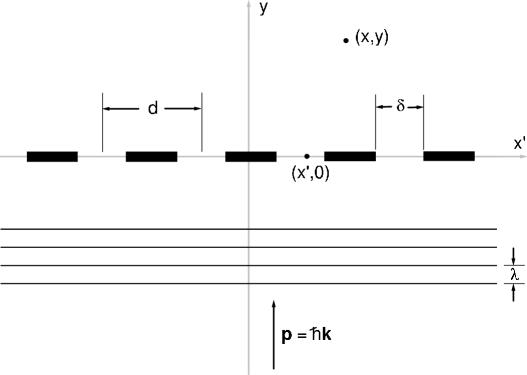
Figure 1: Scheme of the physical system studied. Note that $x^{\prime}$ refers to the coordinate along the grating, while $x$ is the actual coordinate out of the grating.

In Optics it is common to consider sharp-edge slits to study interference and diffraction, as in the model described above. Changing the shape of the initial wave function would not induce significant changes in the momentum distribution. For example, one may use Gaussians instead of square wave functions, i.e., at the openings we have

$$\psi(x,0)\propto e^{-(x-x_{c})^{2}/a^{2}},$$ (6)

where $x_{c}$ is the center of the corresponding opening and $a$ is of the order of the slit width. Then a different multiplicative Gaussian factor appears in the first contribution to the momentum distribution, thus $c(k_{x})$ becoming

$$c(k_{x})\propto e^{-k_{x}^{2}a^{2}/4}\ \!\frac{\sin\left(\frac{k_{x}dn}{2}\right)}{\sin\left(\frac{k_{x}d}{2}\right)}.$$ (7)

For $x\gg x^{\prime}$, the term ${x^{\prime}}^{2}$ can be neglected in the exponential function inside the integral in (4). By doing that, one obtains ref5

$$\psi(x,t)=\sqrt{\frac{m}{2\pi\hbar t}}e^{-i\pi/4}e^{i\frac{x^{2}m}{2\hbar t}}\int_{-\infty}^{\infty}dx^{\prime}\,\psi(x^{\prime},0)e^{-i\frac{x^{\prime}xm}{\hbar t}}.$$ (8)

The integral in (8) is nothing else but the function $c$ defined in (3), taking into account that the variable $xm/\hbar t$ plays the role of $k_{x}$. Therefore, one can write

$$\psi(x,t)=\frac{m}{\hbar t}e^{-i\pi/4}e^{ix^{2}m/2\hbar t}c\left(x\frac{m}{\hbar t}\right).$$ (9)

The wave function (1), where the transverse part is given by (2) or (4), explains in a unified way many effects and properties of particle diffraction and interference ref7 , in particular the Talbot effect. Note that, for a periodic (infinite) grating, the integral in (2) reduces to the sum over discrete momentum values and one can easily see that at integer multiples of $2L_{T}$ ($L_{T}=d^{2}/\lambda$ being the Talbot distance ref8 ; ref8-a ; ref8-b ) the transverse wave function is simply equal to the wave function on the grating. The grating pattern is also repeated at odd multiples of $L_{T}$, but shifted by half a grating period, $d/2$, along $x$-axis.

In the case of a finite grating, an approximate form of the Talbot effect appears ref7 ; ref9 . Namely, in the near field one finds self-images distorted at the ends.

3 Momentum distribution trajectories

Interference experiments with beams such that only one particle is launched at a time have demonstrated that particles accumulate with time on the detection screen, building up an interference pattern after some time. In order to describe the emergence of the interference pattern through an accumulation of single particle events one has to assume that particles move along certain trajectories.

The theoretical investigation of the topology of the trajectories is based on various assumptions. Arsenović et al. ref5 assumed that trajectories were straight lines starting at different positions on the slits. The longitudinal momentum of a particle moving along such a trajectory is equal to the longitudinal momentum of the incident beam that reaches the grating, and the distribution of the transverse momentum of the particles is given by $|\bar{c}(p_{x})|^{2}$. This is why we call these trajectories the momentum distribution (MD) trajectories.

Within the MD approach, a particle can start from any slit; if it has the right transverse momentum, it will reach the chosen detection spot. The expression for the screen arrival probability based on the idea of MD trajectories ref5 reads as

$$\tilde{P}(x,t)=\int_{-\infty}^{+\infty}dk_{x}\int_{-\infty}^{+\infty}dx^{\prime}|c(k_{x})|^{2}|\psi(x^{\prime},0)|^{2}\delta(x-x^{\prime}-\hbar k_{x}t/m).$$ (10)

The total probability can be expressed as a sum of $n$ terms

$$\tilde{P}(x,t)=\sum_{i=1}^{n}\tilde{P}_{i}(x,t),$$ (11)

where

$$\tilde{P}_{i}(x,t)=\frac{1}{n\delta}\int_{m(x-x_{r}^{i})/\hbar t}^{m(x-x_{l}^{i})/\hbar t}|c(k_{x})|^{2}dk_{x}$$ (12)

is the probability that a particle which passed through the $i$-th slit of the grating arrives to a point $(x,y=\hbar kt/m)$ at time $t$. Here $x_{l}^{i}$ and $x_{r}^{i}$ are the coordinates of the left and right edges of the $i$-th slit. Note that, as said in the previous Section, the momentum distribution $c(k_{x})$ depends on the initial wave function chosen. This will only influence the probabilities along the $x$ direction, but not the shape of the MD trajectories.

Numerical calculations for various gratings show ref5 ; ref9 ; ref10 that the distributions $\tilde{P}(x,t)$ and $|\psi(x,t)|^{2}$ are almost identical in the far field. In the near field, both distributions look qualitatively similar, however they differ numerically as well as in certain important details. This is understandable because near the slits the topology of particle trajectories is more complicated than in the far field, where the straight-line approximation works fairly well.

4 Bohmian trajectories

The Bohmian trajectories associated with the state of a single particle, $\Psi(\vec{r},t)$, are determined ref1 from the differential equation (guidance condition)

$$\vec{v}(\vec{r},t)=\frac{d\vec{r}}{dt}=\frac{1}{m}\nabla S(\vec{r},t),$$ (13)

where $S(\vec{r},t)$ is the phase of the wave function written in the polar form, i.e.,

$$\Psi(\vec{r},t)=Re^{iS/\hbar}.$$ (14)

It can be easily shown that

$$\nabla S=\hbar\ \!{\rm Im}\left[\frac{\nabla\Psi}{\Psi}\right].$$ (15)

Hence, according to (1), in our case we have

$$\vec{v}=\frac{d\vec{r}}{dt}=\frac{\hbar}{m}\left\{\vec{i}_{y}k+\vec{i}_{x}{\rm Im}\left[\frac{\partial_{x}\psi(x,t)}{\psi(x,t)}\right]\right\},$$ (16)

where $\partial_{x}=\partial/\partial x$. The equation of motion along the $y$-axis,

$$v_{y}=\frac{dy}{dt}=\frac{\hbar k}{m},$$ (17)

is very simple, and has the solution

$$y=y_{0}+\frac{\hbar k}{m}t.$$ (18)

On the other hand, the equation of motion along the $x$-axis

$$v_{x}=\frac{dx}{dt}=\frac{\hbar}{m}\ \!{\rm Im}\left[\frac{\partial_{x}\psi(x,t)}{\psi(x,t)}\right]$$ (19)

can not be solved analytically for all values of $x$. Unlike MD trajectories, for Bohmian trajectories both their distribution and shape are influenced by the choice of the initial wave function ref3 , although fundamental features still remain.

=3in

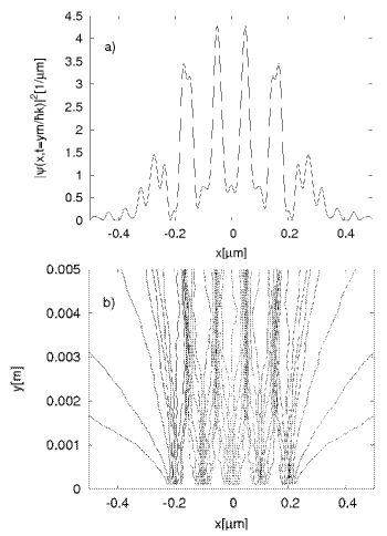
Figure 2: a) Particle distribution function behind a grating with $n$=5 slits for $y$=1.25$L_{T}$, where $L_{T}$ is the Talbot distance $L_{T}$=$d^{2}/\lambda$. b) Trajectories behind a grating with $n$=5 slits for $y\leq 1.25L_{T}$. Trajectories passing through different openings are represented with different line styles. The values of the parameters used in the calculations are: $d=0.1$$\times$10^-6 m, $\delta=0.05$$\times$10^-6 m, $m=1.19$$\times$10^-24 kg, $v=220$ m/s and $\lambda=2.53$$\times$10^-12 m.

Equation (19) can only be solved analytically in the far field, using the approximate expression (9) for $\psi(x,t)$. Using this approximation, Eq. (19) reduces to

$$\frac{dx}{dt}=\frac{x}{t},$$ (20)

whose solution reads

$$x=\frac{x_{0}}{t_{0}}\ \!t.$$ (21)

We have found numerical solutions of Eq. (19) and plotted the Bohmian trajectories for particles behind gratings with $n=5$ and $n=30$ slits. As can be seen in Figs. 1 and 2, the density of Bohmian trajectories at a certain distance from the grating is in good agreement with the quantum mechanical probability density, $|\psi(x,t=ym/\hbar k)|^{2}$, in both the far field (see Fig. 2) and the near field (see Fig. 1). Bohmian trajectories, grouped in bunches, follow the directions that end at the regions of the different intensity peaks. Such an agreement was found previously by Sanz et al. ref1 ; ref3 ; ref4 , who plotted together the intensity pattern obtained by means of the standard quantum mechanics and the histogram obtained by counting Bohmian trajectories (see Fig. 5 in ref4 , for instance).

The consistency of the set of Bohmian trajectories in the near field within the context of the Talbot effect found by Sanz and Miret-Artés ref8 is remarkable. This consistency is also seen in Fig. 3, which shows the Bohmian trajectories behind a grating with $n=30$ slits (only one half of the full pattern is shown; the other half is its mirror image).

=3in

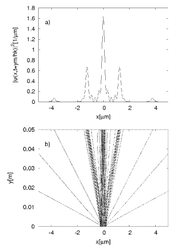
Figure 3: a) Particle distribution function behind a grating with $n$=5 slits for $y$=12.5$L_{T}$, where $L_{T}$ is the Talbot distance $L_{T}$=$d^{2}/\lambda$. b) Trajectories behind a grating with $n$=5 slits for $y\leq 12.5L_{T}$. The values of the parameters used in the calculations are: $d=0.1$$\times$10^-6 m, $\delta=0.05$$\times$10^-6 m, $m=1.19$$\times$10^-24 kg, $v=220$ m/s and $\lambda=2.53$$\times$10^-12 m.

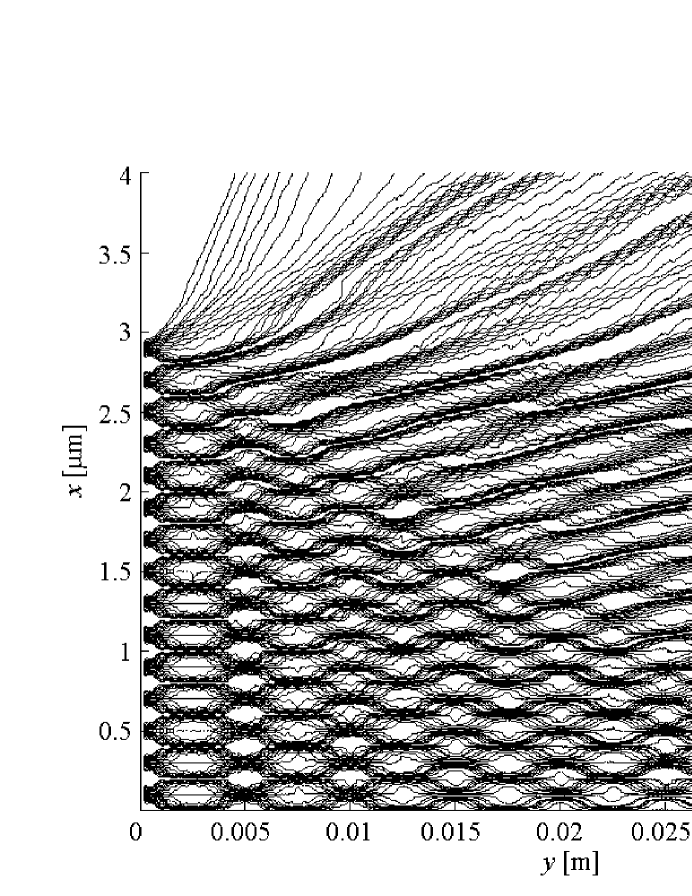
Figure 4: Bohmian trajectories behind one half of a Ronchi grating with $n$=30 slits. The values of the parameters used in the calculations are: $d=0.2$$\times$10^-6 m, $\delta=0.1$$\times$10^-6 m, $k=(\pi/8)$$\times$10¹² m^-1, $m=3.8189$$\times$10^-26 kg and $v=1084$ m/s.

5 Comparison between Bohmian trajectories and MD trajectories

An essential feature of the Bohmian deterministic trajectories is that a particle passing through different slits will not reach the same point on the detection screen. In the far field, Bohmian trajectories asymptotically approach straight lines that connect the center of the grating with the detection spot (see Fig. 4). On the contrary, MD trajectories from different slits may reach the same point on the screen, because this trajectories are associate with different values of transverse momentum. Namely, a particle which leaves certain point at the slit may have various values of momentum, in accordance with the transverse momentum distribution.

=2.5in

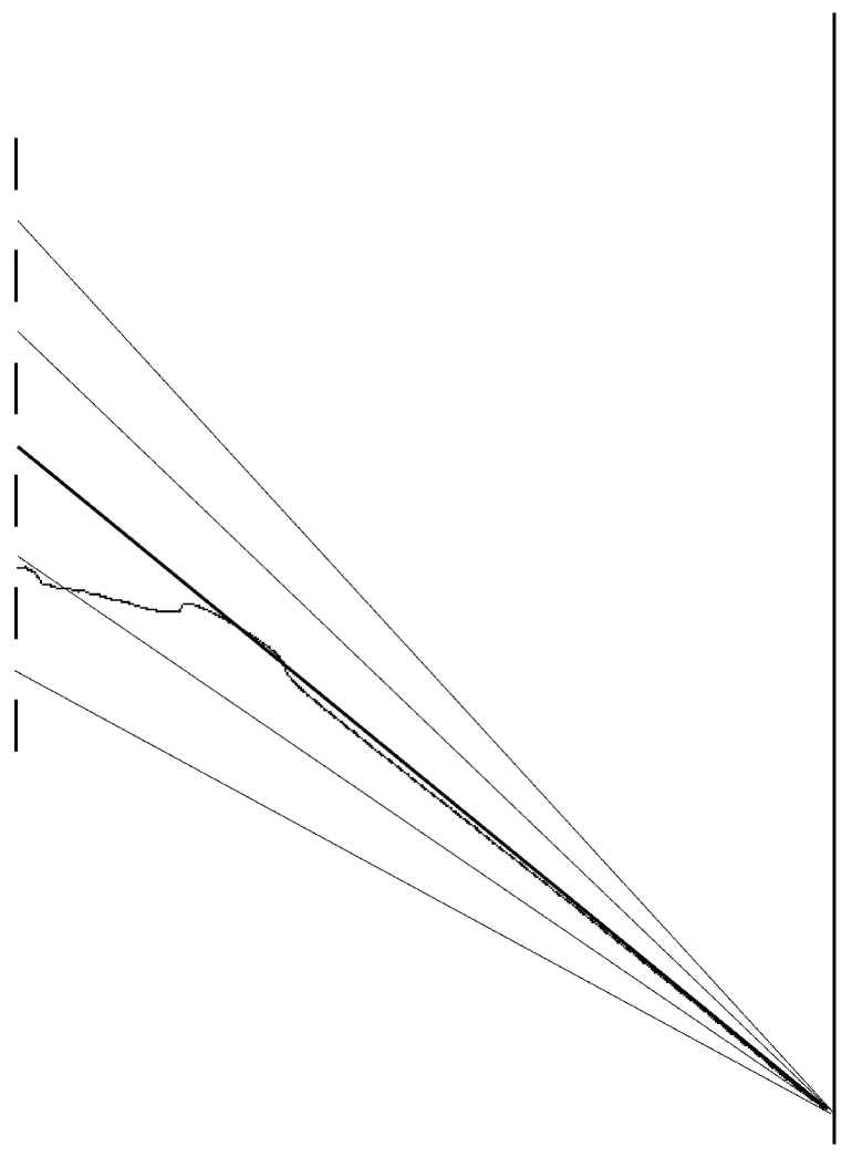
Figure 5: Sketch of MD (five straight lines) and Bohmian (curve) trajectories where there essential features are compared. The central among these straight lines is the asymptote of a Bohmian trajectory.

6 Momentum distribution

It is evident that the probability amplitude of the transverse momenta is an essential feature of the wave function and wave field behind a grating. Thus, the following question arises: is the distribution of transverse momenta associated with Bohmian trajectories identical or different from the distribution $|\bar{c}(p_{x})|^{2}=|c(k_{x})|^{2}/\hbar$, where $c(k_{x})$ is determined by (3)?

Long time ago, based on a general expression for the distribution of Bohmian momenta, Takabayasi ref11 concluded that the aforementioned two distributions were different functions. We have found that this conclusion is not always true. Using the Eq. (19) for Bohmian trajectories, and the approximation (9) for the wave function, we are going to show that the distributions determined from the wave function and from Bohmian trajectories are identical in the far field. In the near field, the distribution of transverse momenta associated with Bohmian trajectories changes with the distance from the grating and is different from the distribution $|\bar{c}(p_{x})|^{2}$.

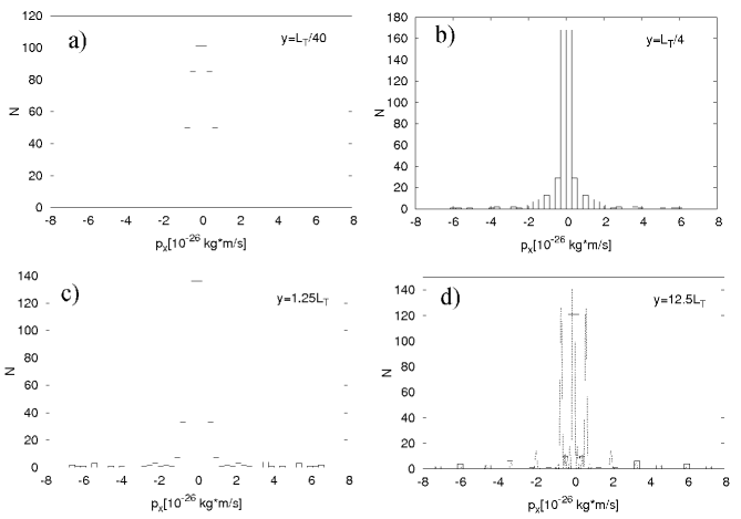
Figure 6: Histogram of the Bohmian momentum distribution at four distances from a grating with $n$=5 slits: (a) $y$=$L_{T}/40$, (b) $y$=$L_{T}/4$, (c) $y$=1.25$L_{T}$ and (d) $y$=12.5$L_{T}$. In panel (d), the quantum momentum distribution has also been plotted with dashed line.

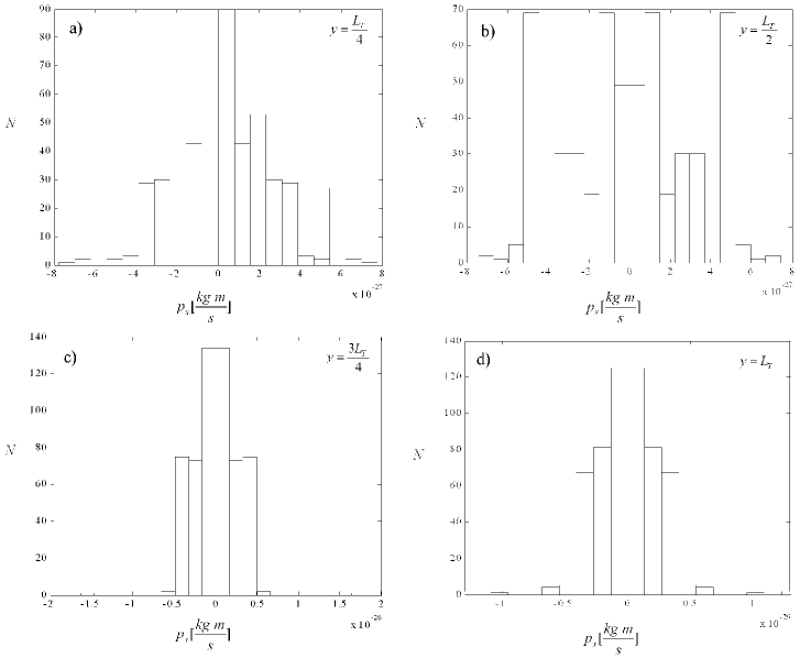
Figure 7: Histogram of the Bohmian momentum distribution at four distances from a grating with $n$=30 slits: (a) $y$=$L_{T}/4$, (b) $y$=$L_{T}/2$, (c) $y$=0.75$L_{T}$ and (d) $y$=$L_{T}$.

An analytical expression for the transverse momentum distribution in the far field can be easily obtained. One starts from a general relation between the probability distribution in the $x$-space and in the $p_{x}$-space,

$$P(x,t)dx=\Pi(p_{x},t)dp_{x}.$$ (22)

Taking into account that $P(x,t)=|\psi(x,t)|^{2}$ as well as relation (19), we find the following expression for the probability distribution of Bohmian momenta along the $x$-axis:

$$\Pi(p_{x},t)=\frac{|\psi(x,t)|^{2}}{\partial_{x}p_{x}}=\frac{|\psi(x,t)|^{2}}{\partial_{xx}S},$$ (23)

where $\partial_{xx}=\partial^{2}/\partial x^{2}$. Using the approximate expression (9) for the transverse wave function, which is valid in the far field, we find:

$$|\psi(x,t)|^{2} = \frac{m}{\hbar t}\left|c\left(x\frac{m}{\hbar t}\right)\right|^{2}$$ (24)

$$\frac{\partial^{2}S}{\partial x^{2}} = \frac{m}{t}.$$ (25)

Therefore, the probability distribution of Bohmian momenta in the far field will be

$$\Pi(p_{x},t)=\frac{1}{\hbar}|c(k_{x})|^{2}=|\bar{c}(p_{x})|^{2}.$$ (26)

We do not have an analytic expression for $\Pi(p_{x},t)$ in the near field, but the histograms of the probability density of Bohmian momenta plotted in Figs. 5 and 6 show that it changes with the distance from the grating. This means that, in the near field, the probability density of Bohmian momenta differs from the momentum distribution $|\bar{c}(p_{x})|^{2}$.

7 Conclusions

By appealing to descriptions in terms of quantum particle trajectories in interference experiments, one can understand how interference patterns emerge from the accumulation of single particle events. This justifies theoretical investigations of properties and statistics of particle trajectories.

In Bohmian mechanics trajectories reproduce exactly the quantum mechanical space distribution in both the far and near fields. The consistency of the set of Bohmian trajectories in the near field within the context of the Talbot effect, demonstrated by Sanz and Miret-Artés ref8 , is remarkable.

The probability amplitude of transverse momenta is also an essential feature of the wave function and the wave field behind the grating. Taking this into account, the following question arises: should particle trajectories comply with the transverse momentum distribution? From our numerical calculations and analytical treatments, it follows that the distributions of transverse momentum determined from the wave function and from Bohmian trajectories are identical in the far field. On the other hand, in the near field, the distribution of transverse momenta associated with the Bohmian trajectories changes with the distance from the grating and is different from the distribution $|\bar{c}(p_{x})|^{2}$.

Considering that the answer to the aforementioned question should be positive, Arsenović et al. proposed ref5 to approximate trajectories by straight lines and to assume that the distribution of particle momenta is determined by the wave function. These trajectories, which we call MD trajectories, reproduce fairly well the quantum mechanical space distribution in the far field ref5 ; ref9 . However, in the near field the agreement is not so satisfactory. It seems that a better agreement of the space distribution derived from MD trajectories with the quantum mechanical space distribution in the near field could be obtained by combining peaces of various Bohmian trajectories ref1 ; ref2 ; ref3 ; ref4 ; ref8 , and by studying also lines of a quantum mechanical current.

- (1) A.S. Sanz, F. Borondo, S. Miret-Artés, Phys. Rev. B 61, 7743 (2000)
- (2) A.S. Sanz, F. Borondo, S. Miret-Artés, Europhys. Lett. 55, 303 (2001)
- (3) A.S. Sanz, F. Borondo, S. Miret-Artés, J. Phys.: Condens. Matter 14, 6109 (2002)
- (4) R. Guantes, A.S. Sanz, J. Margalef-Roig, S. Miret-Artés, Surf. Sci. Rep. 53, 199 (2004)
- (5) D. Arsenović, M. Božić, L. Vušković, J. Opt. B: Quantum Semiclassical Opt. 4, S358 (2002)
- (6) M. Gondran, A. Gondran, Am. J. Phys. 73, 507 (2005)
- (7) M. Božić, D. Arsenović, Acta Physica Hungarica B 26/1-2, 219 (2006)
- (8) A.S. Sanz, S. Miret-Artés, J. Chem. Phys. 126, 234106 (2007)
- (9) M.S. Chapman, C.R. Ekstrom, T.D. Hammond, J. Schmiedmayer, B.E. Tannian, S. Wehinger, D.E. Pritchard, Phys. Rev. A 51 R14 (1995)
- (10) L. Deng, E.W. Hagley, J. Denschlag, J.E. Simsarian, M. Edwards, C.W. Clark, K. Helmerson, S.L. Rolston, W.D. Phillips, Phys. Rev. Lett. 83, 5407 (1999)
- (11) M. Božić, D. Arsenović, L. Vušković, Phys. Rev. A 69, 053618 (2004)
- (12) M. Božić, D. Arsenović, L. Vušković, Concepts of Physics II, 163 (2005)
- (13) T. Takabayasi, Prog. Theor. Phys. 8, 143 (1952)