Equatorial photon motion in the Kerr–Newman spacetimes with a non-zero cosmological constant

Abstract

Discussion of the equatorial photon motion in Kerr–Newman black-hole and naked-singularity spacetimes with a non-zero cosmological constant is presented. Both repulsive and attractive cosmological constants are considered. An appropriate ‘effective potential’ governing the photon radial motion is defined, circular photon orbits are determined, and their stability with respect to radial perturbations is established. The spacetimes are divided into separated classes according to the properties of the ‘effective potential’. There is a special class of Kerr–Newman–de Sitter black-hole spacetimes with the restricted repulsive barrier. In such spacetimes, photons with high positive and all negative values of their impact parameter can travel freely between the outer black-hole horizon and the cosmological horizon due to an interplay between the rotation of the source and the cosmological repulsion. It is shown that this type of behavior of the photon motion is connected to an unusual relation between the values of the impact parameters of the photons and their directional angles relative to outward radial direction as measured in the locally non-rotating frames. Surprisingly, some photons counterrotating in these frames have positive impact parameter. Such photons can be both escaping or captured in the black-hole spacetimes with the restricted repulsive barrier. For the black-hole spacetimes with a standard, divergent repulsive barrier of the equatorial photon motion, the counterrotating photons with positive impact parameters must all be captured from the region near the black-hole outer horizon as in the case of Kerr black holes, while they all escape from the region near the cosmological horizon. Further, the azimuthal motion is discussed and photon trajectories are given in typical situations. It is shown that for some photons with negative impact parameter turning points of their azimuthal motion can exist.

1 Introduction

The Kerr–Newman–de Sitter and Kerr–Newman–anti-de Sitter solutions of Einstein–Maxwell equations represent black holes and naked singularities in spacetimes with a non-zero cosmological constant $\Lambda$. For a repulsive cosmological constant, $\Lambda>0$, the geometry is asymptotically de Sitter, and, generally, contains a cosmological horizon behind which the geometry must be dynamic. For an attractive cosmological constant, $\Lambda<0$, the geometry is asymptotically anti-de Sitter, and can contain black-hole horizons only.

A wide variety of recent cosmological observations, including, e.g., measurements of the present value of the Hubble parameter, measurements of the anisotropy of the cosmic relic radiation, statistics of the gravitational lensing of quasars and active galactic nuclei, and the high-redshift supernovae, suggest that in the framework of the inflationary cosmology a non-zero repulsive cosmological constant $\Lambda>0$ has to be considered seriously in order to explain properties of the presently observed universe [1, 2, 3, 4].

On the other hand, it was recognized recently that the anti-de Sitter spacetime plays an important role in the multidimensional string theory [5, 6, 7]. Therefore, solutions of the Einstein–Maxwell equations with both positive and negative values of the cosmological constant deserve attention.

Properties of the Kerr–Newman spacetimes with a non-zero cosmological constant are appropriately described by their geodesic structure which determines motion of test particles and photons. The motion of photons in the symmetry plane (the equatorial plane) of these spacetimes can be considered as a relatively simple and easily tractable case giving results illustrating the geometric structure in a highly representative way. We shall discuss the properties of the equatorial photon motion for both the black-hole and naked-singularity spacetimes with both the repulsive and attractive cosmological constant.

In Kerr–Newman–de Sitter black-hole spacetimes with appropriately tuned parameters, an unusual effect exists due to the interplay between the rotation of the black hole and the cosmological repulsion [8, 9]; a restricted repulsive barrier of the equatorial photon motion permits photons with sufficiently high positive and all negative values of the impact parameter to move freely between the black hole and cosmological horizons. No such effect exists in the spherically symmetric Schwarzschild–de Sitter and Reissner–Nordström–de Sitter spacetimes, where the repulsive barrier always diverges at the black-hole and cosmological horizons. In Kerr–Newman–de Sitter black-hole spacetimes with a standard, divergent repulsive barrier, the barrier diverges at two radii between the outer black-hole and cosmological horizons. We shall show that the effect of the restricted repulsive barrier is related to the fact that the constants of motion and impact parameter of photons have other asymptotic meaning that we are accustomed to.

The plan of the paper is the following. In Section 2, the radial equation of the equatorial photon motion is discussed. Properties of the radial motion are given in terms of an ‘effective potential’ related to an appropriately defined impact parameter, and circular photon orbits, corresponding to local extrema of the effective potential, are determined for arbitrary values of the parameters of the spacetimes. In Section 3, the Kerr–Newman–de Sitter and Kerr–Newman–anti-de Sitter spacetimes are classified according to the properties of the effective potential of the equatorial photon motion which reflects in an appropriate way the properties of the spacetime geometry. As the criteria for the classification we use the number of event horizons, the number of circular photon orbits, and the number of divergent points of the effective potential. In Section 4, relation between the impact parameter of the equatorial photons and their directional angle relative to the outward radial direction as measured by the family of locally non-rotating observers is determined. The directions corresponding to the captured photons, and the counterrotating photons with positive impact parameter, are established, and related for the Kerr black hole and Kerr–de Sitter black holes with both divergent and restricted repulsive barriers. In Section 5, the azimuthal equation of the equatorial photon motion is considered, and the trajectories of photons are given is some representative cases. Concluding remarks are presented in Section 6.

2 The radial motion

In the standard Boyer–Lindquist coordinates with geometric units ($c=G=1$), the Kerr–Newman geometry with a non-zero cosmological constant $\Lambda$ is described by the line element

$${\rm d}s^{2}= - \frac{\Delta_{r}}{I^{2}\rho^{2}}({\rm d}t-a\sin^{2}\theta\,{\rm d}\phi)^{2}+\frac{\Delta_{\theta}\sin^{2}\theta}{I^{2}\rho^{2}}[a\,{\rm d}t-(r^{2}+a^{2})\,{\rm d}\phi]^{2}$$ (1)

$$+ \frac{\rho^{2}}{\Delta_{r}}\,{\rm d}r^{2}+\frac{\rho^{2}}{\Delta_{\theta}}\,{\rm d}\theta^{2},$$

where

$$\Delta_{r}=\left(1-{\textstyle\frac{1}{3}}\Lambda r^{2}\right)(r^{2}+a^{2})-2Mr+e^{2},$$ (2)

$$\Delta_{\theta}=1+\textstyle{\frac{1}{3}}\Lambda a^{2}\cos^{2}\theta,$$ (3)

$$I=1+{\textstyle\frac{1}{3}}\Lambda a^{2},$$ (4)

$$\rho^{2}=r^{2}+a^{2}\cos^{2}\theta.$$ (5)

Here, $M$ is the mass parameter of the spacetime, $a$ is its specific angular momentum ($a=J/M$), and $e$ is its electric charge. Note that the following analysis of the photon equatorial motion holds for dyonic spacetimes as well, since the magnetic monopole charge $p$ enters the geometry (1) in the same way as the electric charge $e$. Therefore, $e^{2}$ can be simply replaced by $e^{2}+p^{2}$. It is convenient to use dimensionless coordinates and parameters. Therefore, we define a new parameter

$$y={\textstyle\frac{1}{3}}\Lambda M^{2},$$ (6)

and we redefine the following quantities: $s/M\rightarrow s$, $t/M\rightarrow t$, $r/M\rightarrow r$, $a/M\rightarrow a$, $e/M\rightarrow e$, i.e., we express all of these quantities in units of $M$. This is equivalent to putting $M=1$, and leads to

$$\Delta_{r}=(1-yr^{2})(r^{2}+a^{2})-2r+e^{2},$$ (7)

$$\Delta_{\theta}=1+ya^{2}\cos^{2}\theta,$$ (8)

$$I=1+ya^{2};$$ (9)

equation (5) remains the same.

The equations of motion of test particles and photons in the Kerr–Newman spacetimes with a non-zero cosmological constant were in the integrated and separated form given by Carter [10]. Using the results of the discussion of the latitudinal motion [11], the radial equation of motion along equatorial null geodesics can be given in the form (see Eq. (10) in [11])

$$\left(\frac{{\rm d}r}{{\rm d}\lambda}\right)^{2}=\frac{1}{r^{4}}R(r;y,a,e),$$ (10)

with

$$R(r;y,a,e)=I^{2}\left\{[(r^{2}+a^{2})E-a\Phi]^{2}-\Delta_{r}(aE-\Phi)^{2}\right\},$$ (11)

where $E$ and $\Phi$ are the constants of motion connected with symmetries of the geometry (1). They can be expressed as projections of photon’s 4-momentum onto the time Killing vector $\xi_{(t)}={\partial}/{\partial t}$ and the axial Killing vector $\xi_{(\phi)}={\partial}/{\partial\phi}$, respectively; $\lambda$ is the affine parameter along the null geodesics. Recall that the constants of motion $E$ and $\Phi$ cannot here be interpreted as energy and the axial component of the angular momentum at infinity, since the geometry (1) is not asymptotically flat. For the equatorial motion of photons, the last constant of motion, connected with the total angular momentum of the particle, must be restricted by the condition $K=I^{2}(aE-\Phi)^{2}$, due to the equation of the latitudinal motion [11]. In this form it enters the equation of the radial motion (11).

The motion of photons is independent of the constant of motion $E$. The equatorial motion is fully governed by the impact parameter $\ell=\Phi/E$ ($E\neq 0$). However, it is convenient to analyze the radial motion of photons in terms of a redefined impact parameter

$$X\equiv\frac{\Phi}{E}-a=\ell-a.$$ (12)

Then

$$R(r;y,a,e,E,X)=I^{2}E^{2}\left[(r^{2}-aX)^{2}-\Delta_{r}X^{2}\right];$$ (13)

clearly, at the dynamic regions, where $\Delta_{r}<0$, there is $R(r)>0$, and the radial motion has no turning points there. At the stationary regions, where $\Delta_{r}\geq 0$, the turning points of the radial motion, where $R=0$, are determined by the ‘effective potential’

$$X_{\pm}(r;y,a,e)\equiv\frac{r^{2}}{a\mp\sqrt{\Delta_{r}}},$$ (14)

which can be analyzed in a relatively simple way. We will assume $a\geq 0$ in the following.

At the regions, where $a^{2}-\Delta_{r}>0$ (and $X_{+}>0$), the radial motion is allowed, if

$$X>X_{+}(r;y,a,e)\quad\mbox{or}\quad X<X_{-}(r;y,a,e).$$ (15)

At the regions, where $a^{2}-\Delta_{r}<0$ (and $X_{+}<0$), the radial motion is allowed, if

$$X>X_{+}(r;y,a,e)\quad\mbox{and}\quad X<X_{-}(r;y,a,e).$$ (16)

We have to determine the behavior of the effective potential given by the functions $X_{\pm}(r;y,a,e)$. It is necessary to find the regions of reality of the potential, its local extrema and its divergences. We shall use a ‘Chinese boxes’ technique; properties of the potentials are given by families of functions of $r$ and the parameters of the geometry $(y,a,e)$, the properties of these families of functions are given by other families of functions of $r$ with the number of parameters lowered by 1, until we get a function of single $r$. We shall concentrate on the behavior of the potential in the regions of $r>0$.

First, we consider the reality of the effective potential $X_{\pm}(r;y,a,e)$. Clearly, the potential is well defined in the stationary regions ($\Delta_{r}\geq 0$) only. At the boundaries of the stationary regions, if they exist, i.e., at the event horizons of the geometry ($\Delta_{r}=0$), the common points of $X_{+}(r;y,a,e)$ and $X_{-}(r;y,a,e)$ are located. One more common point is at $r=0$; it is the only point where $X_{\pm}=0$. The functions $X_{+}(r;y,a,e)$ and $X_{-}(r;y,a,e)$ have no other zero point. At the horizons ($r=r_{\rm h}$), there is

$$X_{\pm}(r_{\rm h})=\frac{r^{2}_{\rm h}}{a}.$$ (17)

The loci of the event horizons are determined by the condition

$$y=y_{\rm h}(r;a,e)\equiv\frac{r^{2}-2r+a^{2}+e^{2}}{r^{2}\left(r^{2}+a^{2}\right)}.$$ (18)

The function $y_{\rm h}(r;a,e)$ diverges at $r=0$, while it approaches zero from above for $r\rightarrow\infty$. If $a^{2}>0$ and/or $e^{2}>0$, $y_{\rm h}\rightarrow\infty$ for $r\rightarrow 0$. In the special case $a^{2}=e^{2}=0$ (in the Schwarzschild–de Sitter geometry) $y_{\rm h}\rightarrow-\infty$ for $r\rightarrow 0$.

Zeros of the function $y_{\rm h}(r;a,e)$ are determined by the relation

$$a^{2}=a^{2}_{\rm z(h)}(r;e)\equiv 2r-r^{2}-e^{2}.$$ (19)

The function $a^{2}_{\rm z(h)}(r;e)$ determines loci of the horizons of the Kerr–Newman black holes with a zero cosmological constant. Zeros of the function $a^{2}_{\rm z(h)}(r;e)$ are given by the relation

$$e^{2}=e^{2}_{\rm z(z(h))}(r)\equiv r(2-r),$$ (20)

determining loci of the horizons of the Reissner–Nordström black holes. [All the characteristic functions will be denoted in this straightforward, although rather lengthy way. However, this way enables one to obtain an immediate orientation in relations between the families of the characteristic functions.] The maximum of the function $a^{2}_{\rm z(h)}(r;e)$ is at $r=1$, where $a^{2}=1-e^{2}$. This corresponds to the extreme Kerr–Newman black holes. The motion of photons in the Kerr–Newman spacetimes was extensively discussed in [12] and [13].

The local extrema of the function $y_{\rm h}(r;a,e)$ are determined (due to the condition ${\partial y_{\rm h}}/{\partial r}=0$) by the relation

$$a^{2}=a^{2}_{{\rm ex(h)}\pm}(r;e) \equiv \frac{1}{2}\Big{\{}-2r^{2}+r-e^{2}$$ (21)

$$\pm \left.\left[r^{2}(8r+1)-e^{2}\left(4r^{2}+2r-e^{2}\right)\right]^{1/2}\right\}.$$

The reality condition of the functions $a^{2}_{{\rm ex(h)}\pm}(r;e)$ is

$$e^{2} \geq e^{2}_{{\rm r(ex(h))}+},$$ (22)

$$e^{2} \leq e^{2}_{{\rm r(ex(h))}-},$$ (23)

where

$$e^{2}_{{\rm r(ex(h)}\pm)}(r)\equiv r\left\{2r+1\pm 2[r(r-1)]^{1/2}\right\}.$$ (24)

Zero points of $a^{2}_{{\rm ex(h)}\pm}(r;e)$ are determined by the condition

$$e^{2}=e^{2}_{{\rm z(ex(h))}}(r)\equiv{\textstyle\frac{1}{2}}r(3-r).$$ (25)

and the extremal points are given by the relation

$$e^{2}=e^{2}_{{\rm ex(ex(h))}\pm}(r)\equiv\frac{1}{8}r\left\{-16r^{2}+24r+11\pm|4r-1||4r-5|\right\}.$$ (26)

Due to the asymptotic behaviour of $y_{\rm h}(r;a,e)$, at least one event horizon (a cosmological horizon) exists in the spacetimes with $y>0$. If fixed values of $a$ and $e$ permit the existence of local extrema of the function $y_{\rm h}(r;a,e)$, other horizons exist for $y$ located between the local extrema. Therefore, the Kerr–Newman–de Sitter spacetimes can contain two black-hole horizons at $r_{-}$ (the inner one) and $r_{+}$ (the outer one), and a cosmological horizon at $r_{\rm c}$ ($r_{-}<r_{\rm c}<r_{+}$). If the local minimum $y_{\rm min}(a,e)$ enters the region of $y<0$, Kerr–Newman–anti-de Sitter black holes with two horizons at $r_{-}$ and $r_{+}$ can exist, if $y_{\rm min}<y<0$. (Detailed discussion of the properties of the horizons will be presented in the next section.)

The local extrema of the effective potential determine the loci and impact parameters of circular photon orbits. They are given by the condition ${\partial X_{\pm}}/{\partial r}=0$, which implies the equation

$$y^{2}a^{4}r^{4}+2ya^{2}r^{2}(r^{2}+3r-2e^{2})+r^{2}(r^{2}-6r+9+4e^{2})$$

$${}-4r(a^{2}+3e^{2})+4e^{2}(a^{2}+e^{2}) = 0.$$ (27)

The extrema are, therefore, determined by the relation

$$y = y_{{\rm ex}\pm}(r;a,e)\equiv\frac{1}{a^{2}r^{2}}$$ (28)

$$\times \left\{-\left(r^{2}+3r-2e^{2}\right)\pm 2\left[r\left(3r^{2}+a^{2}\right)-e^{2}\left(2r^{2}+a^{2}\right)\right]^{1/2}\right\}.$$

Now, we shall give the relevant properties of the functions $y_{{\rm ex}\pm}(r;a,e)$. For $r\rightarrow\infty$, both $y_{{\rm ex}\pm}\rightarrow-1/a^{2}$. Reality of these functions is determined by the relations

$$a^{2}\left\{\begin{array}[]{ll}\geq a^{2}_{\rm r(ex)}(r;e)&\mbox{if $r\geq e^{2}$}\\ \leq a^{2}_{\rm r(ex)}(r;e)&\mbox{if $r\leq e^{2}$}\end{array}\right.,$$ (29)

where

$$a^{2}_{\rm r(ex)}(r;e)\equiv-\frac{r^{2}\left(3r-2e^{2}\right)}{\left(r-e^{2}\right)}.$$ (30)

The divergence of this function is given by

$$e^{2}=e^{2}_{\rm d(r(ex))}(r)\equiv r,$$ (31)

and $a^{2}_{\rm r(ex)}\rightarrow+\infty(-\infty)$ for $r\rightarrow e^{2}$ from below (above). Zero points of $a^{2}_{\rm r(ex)}(r;e)$ are determined by the relation

$$e^{2}=e^{2}_{\rm z(r(ex))}(r)\equiv{\textstyle\frac{3}{2}}r.$$ (32)

One local extremum of $a^{2}_{\rm r(ex)}$ is at $r=1$ for each $e$, the others are determined by

$$e^{2}=e^{2}_{\rm ex(r(ex))+}\equiv 2r,$$ (33)

$$e^{2}=e^{2}_{\rm ex(r(ex))-}\equiv{\textstyle\frac{3}{4}}r.$$ (34)

One can immediately see that $a^{2}_{\rm r(ex)}<0$ at $r\geq e^{2}$, and the upper reality condition (29) is always satisfied at $r\geq e^{2}$. Thus, we have to consider only the lower reality condition (29), restricted to $r<e^{2}$. There are no divergent points of the functions $y_{{\rm ex}\pm}(r;a,e)$. Their zero points, which determine photon circular orbits of the Kerr–Newman spacetimes, are given by

$$a^{2}=a^{2}_{\rm z(ex)}(r;e)\equiv\frac{\left(r^{2}-3r+2e^{2}\right)^{2}}{4\left(r-e^{2}\right)}.$$ (35)

For divergent points of the function $a^{2}_{\rm z(ex)}$ we find

$$e^{2}=e^{2}_{\rm d(z(ex))}(r) \equiv r$$ (36)

$$= e^{2}_{\rm d(r(ex))}(r),$$

and $a^{2}_{\rm z(ex)}\rightarrow+\infty(-\infty)$ for $r\rightarrow e^{2}$ from above (below). Its zero points are given by

$$e^{2}=e^{2}_{\rm z(z(ex))}(r) \equiv {\textstyle\frac{1}{2}}r(3-r)$$ (37)

$$= e^{2}_{\rm z(ex(h))}(r).$$

One of its extreme points is located at $r=1$ for any value of $e$; the others are given by

$$e^{2}=e^{2}_{{\rm ex(z(ex))}1}(r) \equiv {\textstyle\frac{3}{4}}r$$ (38)

$$= e^{2}_{{\rm ex(r(ex))}-}(r),$$

and

$$e^{2}=e^{2}_{{\rm ex(z(ex))}2}(r) \equiv {\textstyle\frac{1}{2}}r(3-r)$$ (39)

$$= e^{2}_{\rm z(z(ex))}(r)=e^{2}_{\rm z(ex(h))}.$$

Therefore, the zero points of $a^{2}_{\rm z(ex)}(r;e)$ are also extreme points of this function. For $e^{2}=\frac{3}{4}$, there is an inflex point of $a^{2}_{\rm z(ex)}$ at $r=1$. We shall see that the value of $e^{2}=\frac{3}{4}$ plays an important role in the character of the photon equatorial motion. If $e^{2}>\frac{3}{4}$, the function $a^{2}_{\rm z(ex)}$ has no positive extremum at $r<1$, and it has a minimum at $r=1$. If $e^{2}<\frac{3}{4}$, it has a minimum at $r<1$, and a maximum at $r=1$. In the special case of $e^{2}=1$, there is

$$a^{2}_{\rm z(ex)}(r;1)\equiv{\textstyle\frac{1}{4}}(r-1)(r-2)^{2},$$ (40)

and the function $a^{2}_{\rm z(ex)}$ has no divergent points.

Since

$$\frac{\partial y_{{\rm ex}\pm}}{\partial r} = (3r-4e^{2})$$ (41)

$$\times \frac{\left\{\left[r(3r^{2}+a^{2})-e^{2}(2r^{2}+a^{2})\right]^{1/2}\mp(r^{2}+a^{2})\right\}}{a^{2}r^{3}\left[r(3r^{2}+a^{2})-e^{2}(2r^{2}+a^{2})\right]^{1/2}},$$

we can immediately see that the function $y_{{\rm ex}+}(r;a,e)$ has local extrema given by the condition

$$a^{2}=a^{2}_{{\rm ex(ex)}\pm}(r;e) \equiv \frac{1}{2}\Big{\{}-2r^{2}+r-e^{2}$$ (42)

$$\pm \left[r^{2}(8r+1)-e^{2}\left(4r^{2}+2r-e^{2}\right)\right]^{1/2}\Big{\}}$$

$$= a^{2}_{{\rm ex(h)}\pm}(r;e).$$

Therefore, the local extrema of the functions $y_{\rm h}(r,a,e)$ and $y_{{\rm ex}+}(r,a,e)$ coincide. Moreover, both $y_{\rm ex+}(r;a,e)$ and $y_{\rm ex-}(r;a,e)$ have an extreme point determined by the relation

$$e^{2}=e^{2}_{{\rm ex((ex)\pm)}}(r) \equiv {\textstyle\frac{3}{4}}r$$ (43)

$$= e^{2}_{{\rm ex(z(ex))}1}(r)=e^{2}_{{\rm(ex(r(ex))}-}.$$

Clearly, $y_{\rm ex-}(r=\frac{4}{3}e^{2};e)$ is always a minimum. Because the extrema of $y_{\rm ex+}(r,a,e)$ coincide with the extrema of $y_{\rm h}(r,a,e)$ at some $r_{\rm ex(h)}$, we can conclude that if $y_{\rm h}(r;a,e)$ has two extreme points, the function $y_{\rm ex+}(r;a,e)$ has three extreme points. If $y_{\rm ex+}(r=\frac{4}{3}e^{2};e)$ is a maximum, then $y_{\rm ex+}(r=r_{\rm min(h)};e)$ must be a minimum, and circular photon orbits can exist under the inner horizon of black holes (with both $y>0$ and $y<0$). If $y_{\rm ex+}(r=\frac{4}{3}e^{2};e)$ is a minimum, then $y_{\rm ex+}(r=r_{\rm min(h)};e)$ must be a maximum, and two additional circular photon orbits can exist in the field of naked singularities.

It is easy to determine the character of the extreme point of $y_{\rm ex+}(r;a,e)$ at $r=\frac{4}{3}e^{2}$. We can find that at $r=\frac{4}{3}e^{2}$ there is

$$\frac{\partial^{2}y_{{\rm ex}\pm}}{\partial r^{2}}(r={\textstyle\frac{4}{3}}e^{2};e)$$

$$=\frac{3\left\{\left[r(3r^{2}+a^{2})-e^{2}(2r^{2}+a^{2})\right]^{1/2}\mp(r^{2}+a^{2})\right\}}{a^{2}r^{3}\left[r(3r^{2}+a^{2})-e^{2}(2r^{2}+a^{2})\right]^{1/2}},$$ (44)

and, substituting for $r=\frac{4}{3}e^{2}$, the condition

$$\frac{\partial^{2}y_{{\rm ex}\pm}}{\partial r^{2}}(r={\textstyle\frac{4}{3}}e^{2};e)\leq 0,$$ (45)

can be put into the form

$$81a^{4}+9e^{2}(32e^{2}-3)a^{2}+32e^{6}(8e^{2}-9)\geq 0.$$ (46)

The inflex point (${\partial^{2}y_{{\rm ex}\pm}}/{\partial r^{2}}(r=\frac{4}{3}e^{2};e)=0$) is given by the relation

$$a^{2}=a^{2}_{\rm inf\pm}(e)\equiv\frac{1}{18}e^{2}\left[3-32e^{2}\pm\sqrt{3(320e^{2}+3)}\right].$$ (47)

There is $a^{2}_{\rm inf-}(e)<0$ for $e^{2}<0$; zeros of $a^{2}_{\rm inf+}(e)$ are at $e^{2}=0$, and $e^{2}=\frac{9}{8}$. The maximum of this function is

$$a^{2}_{\rm max(inf+)}=0.2666.$$ (48)

The maxima of $y_{\rm ex+}(r;a,e)$ at $r=\frac{4}{3}e^{2}$ (${\partial^{2}y_{{\rm ex}\pm}}/{\partial r^{2}}(r=\frac{4}{3}e^{2};e)<0$) are determined by the conditions

$$a^{2}>a^{2}_{\rm inf+}(e),$$ (49)

$$a^{2}<a^{2}_{\rm inf-}(e),$$ (50)

while for the minima (${\partial^{2}y_{{\rm ex}\pm}}/{\partial r^{2}}(r=\frac{4}{3}e^{2};e)>0$) we arrive at

$$a^{2}_{\rm inf-}<a^{2}<a^{2}_{\rm inf+}.$$ (51)

Finally, let us determine divergent points of the effective potential. Only $X_{+}(r;y,a,e)$ can diverge; the loci of the divergent points are given by the relation

$$y=y_{\rm d}(r;a,e)\equiv\frac{r^{2}-2r+e^{2}}{r^{2}(r^{2}+a^{2})}.$$ (52)

For $r\rightarrow\infty$, this function goes to zero from above; clearly, there is $y_{\rm h}(r;a,e)>y_{\rm d}(r;a,e)$. The divergence of $y_{\rm d}(r;a,e)$ occurs at $r=0$. Notice that if $e^{2}>0$, $y_{\rm d}(r\rightarrow 0)\rightarrow\infty$, while for $e=0$, $y_{\rm d}(r\rightarrow 0)\rightarrow-\infty$. (The case of $e=0$ is discussed in [8].)

Zeros of the function $y_{\rm d}(r;a,e)$ are independent of the parameter $a$;

$$e^{2}=e^{2}_{\rm z(d)}(r) \equiv r(2-r)$$ (53)

$$= e^{2}_{\rm z(z(h))}(r).$$

The local extrema of the function $y_{\rm d}(r;a,e)$ are determined by

$$a^{2}=a^{2}_{{\rm ex(d)}}(r;e)\equiv\frac{r^{2}(r^{2}-3r+2e^{2})}{(r-e^{2})}.$$ (54)

Divergent points of $a^{2}_{{\rm ex(d)}}(r;e)$ are given by

$$e^{2}=e^{2}_{\rm d(ex(d))}(r) \equiv r$$ (55)

$$= e^{2}_{\rm d(r(ex))}(r)=e^{2}_{\rm d(z(ex))}(r).$$

In the special case of $e=1$, there is no divergent point since

$$a^{2}_{\rm ex(d)}(r;1)=r^{2}(r-1).$$ (56)

Zero points of the function $a^{2}_{{\rm ex(d)}}(r;e)$ are located where

$$e^{2}=e^{2}_{\rm z(ex(d))}(r) \equiv {\textstyle\frac{1}{2}}r(3-r)$$ (57)

$$= e^{2}_{\rm z(z(ex))}(r)=e^{2}_{\rm z(ex(h))}(r)=e^{2}_{\rm ex(z(ex))2}(r),$$

and its local extrema are determined by the relation

$$e^{2}=e^{2}_{{\rm ex(ex(d))}\pm}(r)\equiv\frac{1}{8}\left\{-4r^{2}+11r\pm 4r\left|r-\frac{5}{4}\right|\right\}.$$ (58)

Now, we can discuss properties of the photon equatorial motion using the formulae presented above. The properties enable us to classify the spacetimes under consideration.

3 Classification of the spacetimes

We propose a classification of the Kerr–Newman–de Sitter and Kerr–Newman–anti-de Sitter spacetimes according to the properties of the effective potential $X_{\pm}(r;y,a,e)$ governing photon motion in the equatorial plane. The classification will arise from a systematic study of the properties of the functions given in the preceding section. The crucial features of the classification will be the number of event horizons present in these spacetimes, the number of divergences of the effective potential, the number of its local extrema, governing loci and impact parameters of circular photon geodesics, and its asymptotic behavior.

Figure 1: The characteristic functions $e^{2}(r)$ governing the reality conditions (event horizons), local extrema and divergent points of the effective potential of the equatorial photon motion in the Kerr–Newman spacetimes with a non-zero cosmological constant. The functions $e^{2}_{\rm ex(ex(h))\pm}(r)$ are represented by the bold solid curves; their linear part represents also the function $e^{2}_{\rm ex(r(ex))+}(r)$. The functions $e^{2}_{\rm r(ex(h))\pm}(r)$ are represented by the bold dotted curve. The bold dashed-dotted curve represents the functions $e^{2}_{\rm z(ex(h))}(r)=e^{2}_{\rm z(z(ex))}(r)=e^{2}_{\rm ex(z(ex))2}(r)=e^{2}_{\rm z(ex(d))}(r)$. The functions $e^{2}_{\rm ex(ex(d))\pm}(r)$ are represented by the thin solid curves; the linear part of them corresponds also to the functions $e^{2}_{\rm ex(r(ex))-}(r)=e^{2}_{\rm ex(z(ex))1}(r)=e^{2}_{\rm ex((ex)\pm)}(r)$, the parabolic part corresponds also to the functions $e^{2}_{\rm z(z(h))}(r)=e^{2}_{\rm z(d)}(r)$. The function $e^{2}_{\rm z(r(ex))}(r)$ is represented by the thin dotted line. The functions $e^{2}_{\rm d(r(ex))}(r)=e^{2}_{\rm d(z(ex))}(r)=e^{2}_{\rm d(ex(d))}(r)$ are represented by the thin dashed-dotted line. The inflex points of the function $y_{\rm h}(r;a,e)$ are given by the branch of the function $e^{2}_{{\rm ex(ex(h))}-}(r)$ located at $r\geq 1.5$ and $e^{2}\leq\frac{9}{8}$ (emphasized by extra bold curve), where $a^{2}_{{\rm ex(h)}+}(r;e)>0$. The inflex points of $y_{\rm d}(r;a;e)$ are given by the function $e^{2}_{{\rm ex(ex(d))}\pm}(r)$ at $r\geq 1.5$ and $e^{2}\geq\frac{9}{8}$, i.e., outside the region of existence of black-hole horizons.

All the characteristic functions $e^{2}(r)$

• $e^{2}_{\rm r(ex(h))\pm}(r)$,

• $e^{2}_{\rm z(ex(h))}(r)=e^{2}_{\rm z(z(ex))}(r)=e^{2}_{\rm ex(z(ex))2}(r)=e^{2}_{\rm z(ex(d))}(r)$,

• $e^{2}_{\rm ex(ex(h))\pm}(r)$,

• $e^{2}_{\rm z(z(h))}(r)=e^{2}_{\rm z(d)}(r)$,

• $e^{2}_{\rm d(r(ex))}(r)=e^{2}_{\rm d(z(ex))}(r)=e^{2}_{\rm d(ex(d))}(r)$,

• $e^{2}_{\rm z(r(ex))}(r)$,

• $e^{2}_{\rm ex(r(ex))-}(r)=e^{2}_{\rm ex(z(ex))1}(r)=e^{2}_{\rm ex(ex)\pm}(r)$,

• $e^{2}_{\rm ex(ex(d))\pm}(r)$,

• $e^{2}_{\rm ex(r(ex))+}(r)$,

which are relevant in order to determine the properties of the characteristic functions $a^{2}(r;e)$

• $a^{2}_{\rm ex(h)\pm}(r;e)=a^{2}_{\rm ex(ex)\pm}(r;e)$,

• $a^{2}_{\rm z(ex)}(r;e)$,

• $a^{2}_{\rm r(ex)}(r;e)$,

• $a^{2}_{\rm z(h)}(r;e)$,

• $a^{2}_{\rm ex(d)}(r;e)$,

are illustrated in Fig. 1. Of course, we must restrict ourselves to the relevant regions, where the characteristic functions $e^{2}(r)$, and $a^{2}(r;e)$ are non-negative.

Figure 2: The sequence of characteristic functions $a^{2}(r;e)$ determining behavior of functions $y_{\rm h}(r;a;e)$, $y_{\rm ex\pm}(r;a;e)$, $y_{\rm d}(r;a;e)$ characterizing properties of the effective potential of the equatorial photon motion. The functions are drawn in the physically relevant part $a^{2}(r)\geq 0$ only: $a^{2}_{\rm ex(h)}$ are drawn as bold solid curves, $a^{2}_{\rm z(h)}$ as bold dashed curves, $a^{2}_{\rm ex(d)}$ as thin solid curves, $a^{2}_{\rm z(ex)}$ as thin dashed curves, and $a^{2}_{\rm r(ex)}$ as thin dashed-dotted curves. The sequence covers all the qualitatively different cases (A)–(D) of the behavior of the functions $a^{2}(r;e)$ in the dependence on the parameter $e$, as determined in Section 3. The following values of parameter $e$ are used: (a) $e^{2}=0.5$, (b) $e^{2}=0.95$, (c) $e^{2}=1.1$, (d) $e^{2}=1.5$.

Figure 3: The functions $a^{2}_{\rm inf+}(e^{2})$ (bold solid curve), $a^{2}_{\rm ex(z(ex))}(e^{2})$ (bold dashed curve), $a^{2}_{\rm max(z(h))}(e^{2})$ (bold dotted curve), $a^{2}_{\rm max(ex(h))+}(e^{2})$ (thin solid curve), and $a^{2}_{\rm min(ex(d))}(e^{2})$ (thin dashed curve), determining behavior of the functions $y_{\rm h}(r;a,e)$, $y_{\rm ex\pm}(r;a,e)$, $y_{\rm d}(r;a,e)$. Note that the function $a^{2}_{\rm max(z(h))}(e^{2})$ separates the black-hole and naked-singularity Kerr–Newman spacetimes in the parameter space ($a^{2}$-$e^{2}$), and by itself corresponds to Kerr–Newman extreme black holes. Similarly, the function $a^{2}_{\rm ex(z(ex))}(e^{2})$ separates the regions of the Kerr–Newman spacetimes admitting different number of circular photon geodesics. On the other hand, the function $a^{2}_{\rm max(ex(h))+}(e^{2})$ represents the limiting values of parameters $a^{2}$, $e^{2}$ allowing the existence of the Kerr–Newman–de Sitter black holes (with $y$ tuned appropriately); above this function, naked-singularity spacetimes exist for any $y>0$.

It follows from the behavior of the characteristic functions $e^{2}(r)$ that there are four qualitatively different cases of the behavior of the characteristic functions $a^{2}(r;e)$ at the relevant region of $a^{2}\geq 0$. We denote them in the following way:

(A)

$e^{2}<\frac{3}{4}$ ,

(B)

$\frac{3}{4}<e^{2}<1$ ,

(C)

$1<e^{2}<\frac{9}{8}$ ,

(D)

$e^{2}>\frac{9}{8}$.

The behavior of the characteristic functions $a^{2}(r;e)$ is for the cases A–D demonstrated in Figs 2a–d. The limiting situations, corresponding to equalities in conditions A–D, can be inferred in a straightforward way, and are related to continuous changes of these characteristic functions.

The characteristic functions enable us to determine the behavior of the functions $y_{\rm h}(r;a,e)$, $y_{{\rm ex}\pm}(r;a,e)$, $y_{\rm d}(r;a,e)$. However, in order to find the regions of the parameter $a^{2}$ corresponding to different cases of the behavior of $y_{\rm h}$, $y_{\rm ex\pm}$, $y_{\rm d}$, we need the functions $a^{2}_{\rm inf+}(e)$, $a^{2}_{\rm ex(z(ex))}(e)$, $a^{2}_{\rm max(z(h))}(e)$, $a^{2}_{\rm max(ex(h)+)}(e)$, $a^{2}_{\rm min(ex(d))}(e)$, which are drawn in Fig. 3. The function $a^{2}_{\rm inf+}(e)$ is given by the relation (47). Further, we can easily find that for the extreme point of $a^{2}_{\rm z(ex)}(r;e)$ at $r=\frac{4}{3}e^{2}$ there is

$$a^{2}_{\rm ex(z(ex))}(e)\equiv{\textstyle\frac{1}{27}}e^{2}(8e^{2}-9)^{2},$$ (59)

and for $a^{2}_{\rm z(h)}(r;e)$ at $r=1$ there is

$$a^{2}_{\rm max(z(h))}(e)\equiv 1-e^{2}.$$ (60)

Clearly, $a^{2}_{\rm max(z(h))}(e)$ governs the extremal Kerr–Newman black holes, and, together with the function $a^{2}_{\rm ex(z(ex))}(e)$ yields the classification of the equatorial photon motion in the Kerr–Newman backgrounds [12, 13]. The function $a^{2}_{\rm max(ex(h))+}(e)$ is implicitly given in a parametric form by $a^{2}_{\rm ex(h)+}(r;e)$, and $e^{2}_{\rm ex(ex(h))-}(r)$ with $r$ being the parameter. Similarly, the function $a^{2}_{\rm min(ex(d))}(e)$ is determined by $a^{2}_{\rm ex(d)}(r;e)$, and $e^{2}_{\rm ex(ex(d))+}(r)$; we find

$$a^{2}_{\rm min(ex(d))}(e)\equiv 2\left({\textstyle\frac{2}{3}}\right)^{5}e^{6}(8e^{2}-9)^{2}.$$ (61)

Further, it is useful to establish the common points of $y_{\rm ex+}(r;a,e)$ and $y_{\rm d}(r;a,e)$. They are determined by two conditions:

$$e^{2}=e^{2}_{\rm(d\hbox{-}ex)+}(r;a)\equiv\frac{a^{2}r+r^{3}(3-r)}{2r^{2}+a^{2}},$$ (62)

$$e^{2}=e^{2}_{\rm(d\hbox{-}ex)-}(r;a)\equiv\frac{-4a^{4}+a^{2}r(1-4r)+r^{3}(3-r)}{2r^{2}+a^{2}}.$$ (63)

However, the condition (54) for the extrema of $y_{\rm d}(r;a,e)$ can be transferred into the form

$$e^{2}_{\rm ex(d)}(r;a)\equiv\frac{a^{2}r+r^{3}(3-r)}{2r^{2}+a^{2}}.$$ (64)

Clearly, the intersections determined by the first condition (62) are just at the extrema of the function $y_{\rm d}(r;a,e)$. The intersections determined by the second condition (63) are irrelevant for the character of the photon equatorial motion.

Now, using Figs 2 and 3, the behavior of the functions $y_{\rm h}(r;a,e)$, $y_{{\rm ex}\pm}(r;a,e)$, $y_{\rm d}(r;a,e)$ can be given in the following exhaustive scheme. [However, we must stress that in some of the following cases, there are variants of the behavior of these functions, determined by different relations between their extremal values than are those shown in the corresponding figures. These variant cases will not be drawn explicitly. We will only point out, which variants should be considered in the explicitly illustrated cases.]

(A)

$e^{2}<3/4$

(a)

$a^{2}<a^{2}_{\rm inf+}$ (Fig. 4a)

(b)

$a^{2}_{\rm inf+}<a^{2}<a^{2}_{\rm ex(z(ex))}$ (Fig. 4b)

(c)

$a^{2}_{\rm ex(z(ex))}<a^{2}<a^{2}_{\rm max(z(h))}=1-e^{2}$ (Fig. 4c)

(d)

$1-e^{2}=a^{2}_{\rm max(z(h))}<a^{2}<a^{2}_{\rm max(ex(h))+}$ (Fig. 4d)

(e)

$a^{2}_{\rm max(ex(h))+}<a^{2}$ (Fig. 4e)

In the case Aa one has to compare $y_{\rm min(d)}(a,e)$ with $y_{\rm min(ex+)(a,e)}$. The function $y_{\rm min(d)}(a,e)$ is given implicitly in a parametric way by $a^{2}_{\rm ex(d)}(r;e)$ and $y_{\rm d}(r;a,e)$, with $r$ being the parameter. On the other hand, at $r=\frac{4}{3}e^{2}$ the minima of $y_{{\rm ex}\pm}(r;a,e)$ at $r=\frac{4}{3}e^{2}$ (or maximum of $y_{\rm ex+}$, for $a^{2}>a^{2}_{\rm inf+}$) are determined by the functions

$$y_{{\rm ex(ex)}\pm}(a,e)\equiv\frac{9}{8a^{2}e^{2}}\left[-1-\frac{8e^{2}}{9}\pm\left(\frac{32e^{2}}{9}+\frac{a^{2}}{3e^{2}}\right)^{1/2}\right].$$ (65)

The minimum $y_{\rm min(ex)+}(a,e)$ and maxima $y_{\rm max(ex)+}(a,e)$ are separated by the function $a^{2}_{\rm inf+}(e)$. In the case Ac the function $y_{\rm max(ex+)}(a,e)$ have to be related with $y_{\rm max(d)}(a,e)$ and $y_{\rm max(h)}(a,e)$, while in the case Ad, all the functions $y_{\rm max(ex+)}(a,e)$, $y_{\rm max(d)}(a,e)$, $y_{\rm min(h)}(a,e)$, and $y_{\rm max(h)}(a,e)$ have to be related. The function $y_{\rm max(d)}(a,e)$ is parametrically given by $a^{2}_{\rm ex(d)}(r;e)$ and $y_{\rm d}(r;a,e)$. The functions $y_{\rm min(h)}(a,e)$ and $y_{\rm max(h)}(a,e)$ are parametrically given by $a^{2}_{\rm ex(h)+}(r;e)$ and $y_{{\rm h}}(r;a,e)$. All these functions are determined by a numerical code.

(B)

$3/4<e^{2}<1$

(a)

$a^{2}<a^{2}_{\rm max(z(h))}=1-e^{2}$ (equivalent to Aa)

(b)

$1-e^{2}=a^{2}_{\rm max(z(h))}<a^{2}<a^{2}_{\rm ex(z(ex))}$ (Fig. 4f)

(c)

$a^{2}_{\rm ex(z(ex))}<a^{2}<a^{2}_{\rm inf+}$ (Fig. 4g)

(d)

$a^{2}_{\rm inf+}<a^{2}<a^{2}_{\rm max(ex(h))+}$ (equivalent to Ad)

(e)

$a^{2}_{\rm max(ex(h))+}<a^{2}$ (equivalent to Ae)

In the case Bb, $y_{\rm min(d)}(a,e)$ have to be related to $y_{\rm min(ex+)}(a,e)$, and $y_{\rm min(h)}(a,e)$ to $y_{\rm max(d)}(a,e)$, while in the case Bc we have to relate $y_{\rm max(d)}(a,e)$ to $y_{\rm min(h)}(a,e)$, and $y_{\rm min(ex+)}(a,e)$ to $y_{\rm max(d)}(a,e)$.

(C)

$1<e^{2}<9/8$

(a)

$a^{2}<a^{2}_{\rm ex(z(ex))}$ (Fig. 4h)

(b)

$a^{2}_{\rm ex(z(ex))}<a^{2}<a^{2}_{\rm inf+}$ (Fig. 4i)

(c)

$a^{2}_{\rm inf+}<a^{2}<a^{2}_{\rm max(ex(h))}$ (Fig. 4j)

(d)

$a^{2}_{\rm max(ex(h))+}<a^{2}$ (equivalent to Ae)

In the case Ca we have to relate $y_{\rm min(h)}(a,e)$ to $y_{\rm max(d)}(a,e)$; in the case Cb we should consider relations of $y_{\rm min(h)}(a,e)$ with $y_{\rm max(d)}(a,e)$, and of $y_{\rm min(ex+)}(a,e)$ with $y_{\rm min(d)}(a,e)$ and $y_{\rm max(d)}(a,e)$; in the case Cc we have to relate $y_{\rm min(h)}(a,e)$ to $y_{\rm max(d)}(a,e)$, and $y_{\rm max(ex+)}(a,e)$ to $y_{\rm max(h)}(a,e)$.

(D)

$9/8<e^{2}$

(a)

$a^{2}<a^{2}_{\rm min(z(ex))}$ (Fig. 4k)

(b)

$a^{2}_{\rm min(z(ex))}<a^{2}<a^{2}_{\rm min(ex(d))}$ (Fig. 4l)

(c)

$a^{2}_{\rm min(ex(d))}<a^{2}$ (equivalent to Ae)

There is no variant in these cases. Note that in the special case of $e=1$, the cases Ca–d are relevant with

$$y_{\rm d}(r;a,e)=\frac{(r-1)^{2}}{r^{2}(r^{2}+a^{2})}.$$ (66)

By using the classification criteria presented in the beginning of this section, we can show that there is 18 types of the behavior of the effective potential $X_{\pm}(r;y,a,e)$. We shall characterize all the classes, and the corresponding behavior of the effective potential. However, we shall determine and illustrate the corresponding range of the parameters $y,a,e$ only for some selected classes. Of course, using the same procedure as for the selected classes, the corresponding distribution in the parameter space can be determined also for the remaining classes. We shall concentrate on the detailed distribution of the black-hole spacetimes, and will not consider the naked-singularity spacetimes.

(a)

(b)

(c)

(d)

(e)

(f)

(g)

(h)

(i)

(j)

(k)

(l)

Figure 4: Different types of the functions $y_{\rm h}(r;a,e)$ (dotted curves), $y_{\rm ex\pm}(r;a,e)$ (solid curves), $y_{\rm d}(r;a,e)$ (dashed curves) determining the behavior of the ‘effective potential’ of the photon equatorial motion. The cases illustrated in figures (a)–(l) are governed by the behavior of the functions $a^{2}(r)$ and $a^{2}(e^{2})$; see Section 3, where the situations not explicitly illustrated by the sequence of figures (a)–(l) are discussed. (a) $e^{2}=0.5$, $a^{2}=0.16$, (b) $e^{2}=0.5$, $a^{2}=0.36$, (c) $e^{2}=0.5$, $a^{2}=0.49$, (d) $e^{2}=0.5$, $a^{2}=0.64$, (e) $e^{2}=0.5$, $a^{2}=0.81$, (f) $e^{2}=0.95$, $a^{2}=0.06$, (g) $e^{2}=0.95$, $a^{2}=0.1$, (h) $e^{2}=1.1$, $a^{2}=0.001$, (i) $e^{2}=1.1$, $a^{2}=0.01$, (j) $e^{2}=1.1$, $a^{2}=0.02$, (k) $e^{2}=1.5$, $a^{2}=0.1$, (l) $e^{2}=1.5$, $a^{2}=4$.

The starting point of our classification is separation of Kerr–Newman–de Sitter ($y>0$) and Kerr–Newman–anti-de Sitter ($y<0$) spacetimes. This basic separation reflects different asymptotic character of these spacetimes, which is represented by different asymptotic behavior of $X_{\pm}(r;y,a,e)$. For $y>0$, a cosmological horizon exist behind which the spacetime is dynamic. The effective potential is well-defined up to the cosmological horizon. For $y<0$, there is no cosmological horizon, and for $r\rightarrow\infty$ there is

$$X_{\pm}\approx\pm\frac{1}{\sqrt{-y}}.$$ (67)

Further, we have to separate the black-hole and naked-singularity spacetimes, i.e., we use the criterion of the number of event horizons representing reality limits of the effective potential. We give the discussion in full detail – the other cases will be considered in much briefer form. The event horizons are determined by the function $y_{\rm h}(r;a,e)$. Due to the behavior of this function at $r\rightarrow 0$ and $r\rightarrow\infty$, at least one event horizon (cosmological) exist in spacetimes with $a^{2}>0$, $e^{2}>0$. The black-hole horizons can exist, if $y_{\rm h}(r;a,e)$ has local extrema. The relevant extrema of $a^{2}_{{\rm ex(h)}+}(r;e)$ are given by $e^{2}_{{\rm ex(ex(h))}-}(r)$ at the branch lying under the curve $e^{2}_{{\rm z(ex(h))}}$. Therefore, the relevant extrema of $a^{2}_{{\rm ex(h)}+}(r;e)$ exist for $e^{2}<\frac{9}{8}$. In the limiting case of $e=0$, the function $a^{2}_{{\rm ex(h)}+}(r)$ has its maximum at $r_{\rm crit}=1.61603$, with a corresponding critical value of the rotation parameter corresponding to the marginal black-hole spacetime

$$a^{2}_{\rm crit}=\left(\frac{3+2\sqrt{3}}{8}\right)\sqrt{\left(7+4\sqrt{3}\right)}-\frac{\sqrt{3}}{16}\left(5\sqrt{3}+8\right)=1.21202,$$ (68)

and the critical value of the cosmological parameter

$$y_{\rm crit}=\frac{16\left[\sqrt{\left(7+4\sqrt{3}\right)}-3\right]}{3\left(7+4\sqrt{3}\right)\left[\sqrt{7+4\sqrt{3}}+1\right]}=0.0592.$$ (69)

If $0<e^{2}<\frac{9}{8}$, the critical value $a^{2}_{\rm max(ex(h))}(e)$, governing an inflex point of $y_{\rm h}(r;a,e)$, is determined by $e^{2}_{{\rm ex(ex(h))}-}(r)$. For $a^{2}<a^{2}_{\rm max(ex(h))}(e)$, the function $y_{\rm h}(r;a,e)$ has two local extrema $y_{\rm min(h)}(a,e)$ and $y_{\rm max(h)}(a,e)$, determined by (21) and (18), with a given value of the parameter $e$. For $a^{2}=a^{2}_{\rm max(ex(h))}(e)$, these extrema coincide at $y_{\rm crit}(e)$ which is the limiting value for black-hole spacetimes with a fixed parameter $e$. The black-hole spacetimes exist for $y_{\rm h(min)}(a,e)<y<y_{\rm h(max)}(a,e)$. If $y=y_{\rm min(h)}(a,e)$, the two black-hole horizons coincide and the geometry determines an extreme black hole; for $y<y_{\rm min(h)}(a,e)$ it determines a naked singularity. Certain kind of ‘instability’ occurs at $y_{\rm max(h)}(a,e)$. If $y=y_{\rm max(h)}(a,e)$, the outer black-hole and cosmological horizons coincide, keeping the role of the cosmological horizon in a spacetime with an extreme black hole. For $y>y_{\rm max(h)}(a,e)$, the geometry describes a naked singularity, and the cosmological horizon is determined be the branch of $y_{\rm h}(r;a,e)$ determining the inner black-hole horizon for $y<y_{\rm max(h)}(a,e)$. The Kerr–Newman–anti-de Sitter black holes correspond to the range of parameters

$$y_{\rm min(h)}(a,e)<y<0.$$ (70)

Distribution of black-hole and naked-singularity spacetimes in the parameter space is given by the functions $y_{\rm min(h)}(a,e)$, $y_{\rm max(h)}(a,e)$, and can be determined by a numerical code. The results are given in Fig. 5. We can see that black-hole spacetimes can exist for all values of the attractive cosmological constant ($y<0$), contrary to the case of repulsive cosmological constant ($y>0$), when black-hole spacetimes must have $y\leq\frac{2}{27}$. The extremal value of $y=\frac{2}{27}$ corresponds to the extreme Reissner–Nordström–de Sitter geometry with the extremal value of $e^{2}=\frac{9}{8}$ (and $a^{2}=0$) [8].

Figure 5: Parameter space ($y$-$a^{2}$-$e^{2}$) of the Kerr–Newman spacetimes with a non-zero cosmological constant separated into parts corresponding to the black-hole and naked-singularity spacetimes, respectively. The boundary between these states is given by the functions $y_{\rm max(h)}(a,e)$ and $y_{\rm min(h)}(a,e)$ determined by a numerical code. The black-hole spacetimes can exist for any asymptotically anti-de Sitter spacetime ($y<0$), while for de Sitter spacetimes ($y>0$), they are restricted by the upper limit $y_{\rm max}=2/27$. In the limiting case, $y=y_{\rm max}$, we obtain a Reissner–Nordström–de Sitter extreme black hole with $e^{2}=9/8$ (and $a^{2}=0$).

Note that in the special case of the Schwarzschild spacetimes ($a^{2}=e^{2}=0$) with $y\neq 0$, there is $y_{\rm h}\rightarrow-\infty$ for $r\rightarrow 0$. Then the black-hole and cosmological horizon exist for $0<y<y_{\rm crit}=\frac{1}{27}$. They are determined by the relations

$$r_{\rm h}=\frac{2}{\sqrt{3y}}\,\cos\frac{\pi+\xi}{3},$$ (71)

$$r_{\rm c}=\frac{2}{\sqrt{3y}}\,\cos\frac{\pi-\xi}{3},$$ (72)

where

$$\xi=\cos^{-1}\left(3\sqrt{3y}\right).$$ (73)

If $y>\frac{1}{27}$, the spacetime is dynamic at all $r>0$, and represents certain kind of naked singularity. On the other hand, in any Schwarzschild–anti-de Sitter geometry with $y<0$ there is a black-hole horizon located at $r_{\rm h}$ determined by the relation

$$r_{\rm h}=\left(-\frac{1}{y}\right)^{1/3}$$

$$\times\left\{\left[1+\left(1-\frac{1}{27y}\right)^{1/2}\right]^{1/3}+\left[1-\left(1-\frac{1}{27y}\right)^{1/2}\right]^{1/3}\right\}.$$ (74)

Clearly, $r_{\rm h}\rightarrow 2$ for $y\rightarrow 0$, while $r_{\rm h}\rightarrow 0$ for $y\rightarrow-\infty$.

The other criterion of the classification is given by the number of divergent points of the effective potential $X_{\pm}(r;y,a,e)$. There exist Kerr–Newman–de Sitter black-hole spacetimes with an unusual property of the effective potential, namely with a restricted repulsive barrier allowing photons with high positive-valued and any negative-valued impact parameter $X$ to move freely between the outer black-hole and cosmological horizons. These spacetimes were extensively studied in [9]. Their character is a non-standard one, because from the photon motion in other black-hole spacetimes we are accustomed to the existence of a divergent barrier repelling photons with high values of impact parameter. Really, if $y=0$, the effective potential diverges at the horizons and at infinity in the spherically symmetric Schwarzschild and Reissner–Nordström black-hole spacetimes. When the rotation is ‘switched on’, i.e., in the Kerr and Kerr–Newman black-hole spacetimes, the effective potential is finite at the horizons, but it diverges at infinity and at some loci between the horizon and infinity. In the case of spherically symmetric Schwarzschild–de Sitter and Reissner–Nordström–de Sitter geometries, the effective potential diverges at the horizons again, as can be inferred directly from the formula

$$X_{\pm}(r;y,e)=\mp\frac{r^{2}}{\sqrt{\Delta_{r}}}.$$ (75)

Therefore, in all these cases, a repulsive barrier does exist for photons with a high magnitude of the impact parameter.

The black-hole spacetimes with a restricted repulsive barrier must have the cosmological-constant parameter in the interval

$$y_{\rm max(d)}(a,e)<y<y_{\rm max(h)}(a,e).$$ (76)

Using a numerical code, the region of the parameter space corresponding to these spacetimes can be determined. The result is shown in Fig. 6.

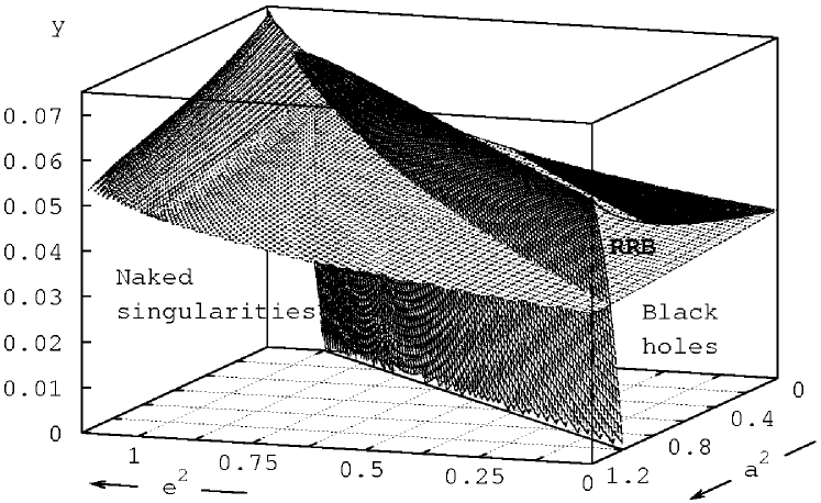
Figure 6: Parameter space of the Kerr–Newman–de Sitter black-hole spacetimes separated into classes Ia+IIa (with divergent repulsive barrier) and Ib+IIb (with restricted repulsive barrier, see below). The boundary surface, determined by a numerical code, is given by the function $y_{\rm max(d)}(a,e)$ illustrated by the light surface.

Extension of the region of the parameter space corresponding to the Kerr–Newman–de Sitter black-hole spacetimes with the restricted repulsive barrier of the photon motion depends strongly on the parameter $e$. The region is suppressed with increasing values of $e$, and it disappears for $e^{2}>\frac{9}{8}$. We can easily find [8] that, for $a=0$, the critical value $y_{\rm crit}(e)$, corresponding to the boundary between the black-hole and naked-singularity spacetimes, shifts from the value $y_{\rm crit}(e=0)=\frac{1}{27}$ for the extreme Schwarzschild–de Sitter geometry to the value $y_{\rm crit}(e^{2}=\frac{9}{8})=\frac{2}{27}$ for the extreme Reissner–Nordström–de Sitter geometry. We can intuitively expect such kind of behavior. Since the rotation parameter $a$ is responsible for the existence of the restricted repulsive barrier, we understand that the corresponding region of the parameter space will be largest for the smallest restrictions coming from the other parameter $e$. The minimal values of the parameter $y$, allowing the black-hole spacetimes with the restricted repulsive barrier are given by the common points of $y_{\rm max(d)}(a,e)$ and $y_{\rm min(h)}(a,e)$. If $e=0$, it reaches its minimum value

$$y_{\rm rrb(min)}(e=0)=0.033185,$$ (77)

at the rotation parameter

$$a^{2}_{\rm rrb(max)}(e=0)=1.08316.$$ (78)

With $e$ increasing, the value of $y_{\rm rrb(min)}(e)$ also increases, while $a^{2}_{\rm rrb(min)}(e)$ decreases. Further, we should note that inspecting the geometries allowing the restricted repulsive barrier, we find that the radii of their outer black-hole and cosmological horizons must be comparable (see Fig. 7).

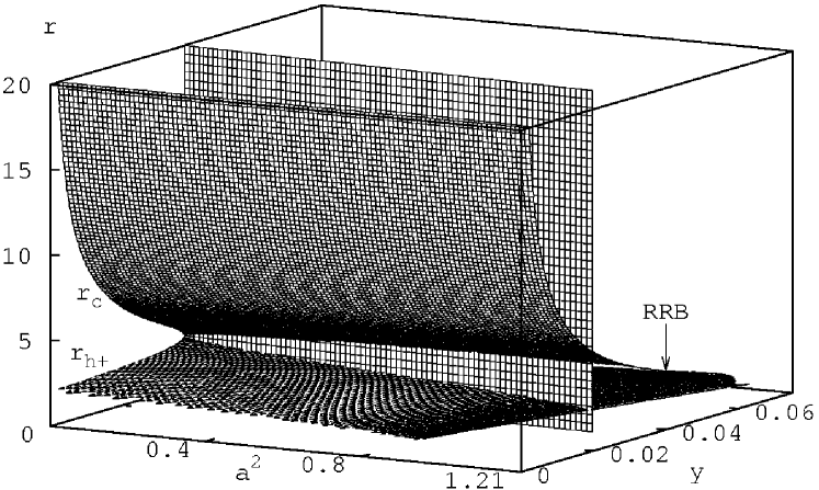
Figure 7: Illustration of dependence of the outer black-hole and cosmological horizon radii of the Kerr–Newman–de Sitter spacetimes with a restricted repulsive barrier on cosmological parameter $y$ and rotation parameter $a^{2}$. The light plane separates the Kerr–de Sitter spacetimes with divergent and restricted repulsive barrier. The cosmological parameter $y$ is so high for these spacetimes that the horizon radii are comparable.

The values of $y_{\rm rrb(min)}(e)$ are very high, and correspond to black holes with an enormously high mass parameter. Considering the recent estimate [4, 14] on the relict cosmological constant

$$\Lambda_{0}\sim 8\pi\times 0.65\,\rho_{\rm crit}\sim 1.1\times 10^{-56}\,{\rm cm}^{-2},$$ (79)

we obtain the limit on the mass of black holes with restricted repulsive barrier to be

$$M\geq M_{\rm rrb(0)}\sim 2\times 10^{22}M_{\odot}.$$ (80)

Of course, radically different estimates on the mass $M_{\rm rrb}$ could be obtained for primordial black holes in the very early stages of expansion of the Universe, when phase transitions connected to symmetry breaking of physical interactions due to Higgs mechanism could take place. For example, the electroweak symmetry breaking at $T\sim 100$ GeV could correspond to an effective cosmological constant [16]

$$\Lambda_{\rm ew}\sim 0.028\,{\rm cm}^{-2},$$ (81)

and the related limiting mass is

$$M_{\rm rrb(ew)}\sim 2.5\times 10^{28}\,{\rm g}\sim 1.3\times 10^{-5}M_{\odot}.$$ (82)

The phenomenon of the restricted repulsive barrier is related to the fact that, similarly to the constants of motion $E$ and $\Phi$, also the impact parameters $X$ or $\ell$ have other asymptotical meaning than we are accustomed to because of the asymptotically de Sitter structure of the spacetimes. Nevertheless, the physical meaning of the impact parameters $X$ and $\ell$ can be given by their relation to directional angles as measured by physically well defined stationary observers located between the black-hole and cosmological horizons. It will be shown in the next section, how directional angles of captured and escaping photons measured by locally non-rotating observers, are related to the impact parameters having positive values for photons counterrotating relative to these observers.

The last criterion for the classification of Kerr–Newman spacetimes with $\Lambda\neq 0$ is given by the local extrema of the effective potential, i.e., it is given by the number of the circular geodesics.

The behavior of the functions $y_{{\rm ex}\pm}(r;a,e)$ implies that there are 0, 2, or 4 circular photon orbits present in the Kerr–Newman spacetimes with $y\neq 0$, except the situations corresponding to the existence of inflex point of these functions. Because the local extrema of the functions $y_{\rm h}(r,a,e)$ and $y_{{\rm ex}+}(r,a,e)$ coincide, we can conclude that in spacetimes with both $y>0$ and $y<0$ two circular photon orbits always exist outside the outer black-hole horizon. Two additional circular photon orbits can exist under the inner black-hole horizon. On the other hand, in the field of naked singularities, there can exist no, two, or four circular photon orbits. Stability of the photon circular orbits against radial perturbation can be directly inferred from the effective potential.

Now, we give the summary of the classification of the Kerr–Newman spacetimes with $y\neq 0$ according to the properties of the ‘effective potential’. We make the basic separation according to the asymptotic character of the spacetime (and the potential). The numbers of the event horizons and circular photon orbits are considered as main criteria of the classification. The divergent points of the effective potential are used as an additional criterion.

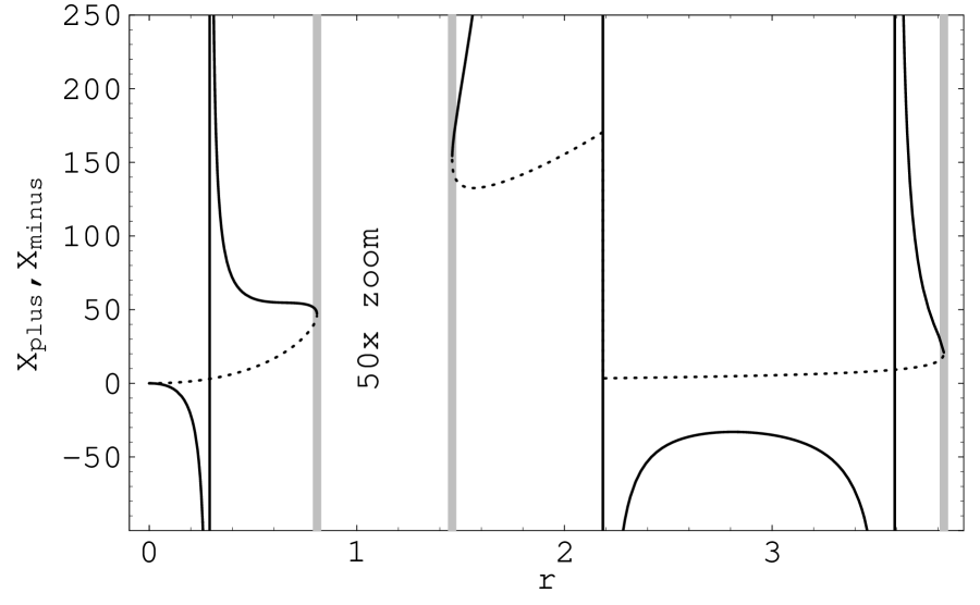
(a) Ia: $y=0.036$, $a^{2}=0.49$, $e^{2}=0.5$

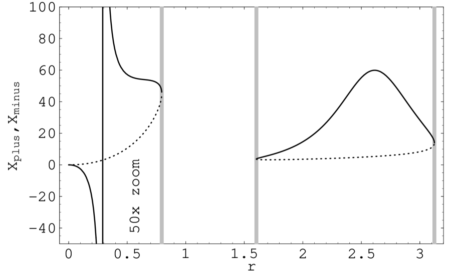
(b) Ib: $y=0.045$, $a^{2}=0.49$, $e^{2}=0.5$

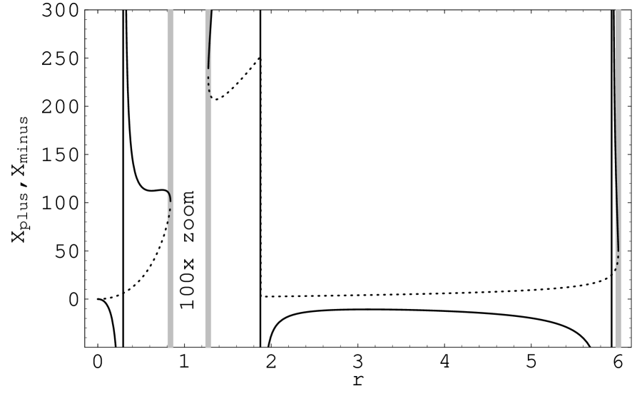
(c) IIa: $y=0.019$, $a^{2}=0.49$, $e^{2}=0.5$

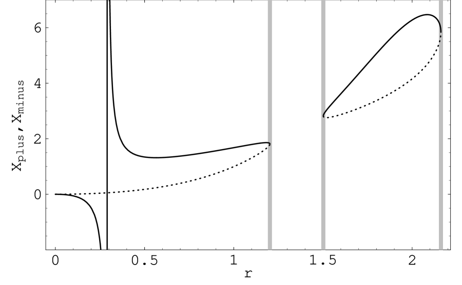
(d) IIb: $y=0.06$, $a^{2}=0.64$, $e^{2}=0.5$

Figure 8: Typical behavior of effective potential $X_{\pm}$ for Kerr–Newman–de Sitter black-hole spacetimes. Stability of the photon circular geodesics can easily be inferred from the character of the effective potential. The vertical bars of the same thickness as the curves are the vertical asymptotes at the points of divergence, the horizons are depicted as thick gray bars. In order to clearly display the structure of the curves (especially the existence/nonexistence of extremes), certain portions of them are vertically zoomed.

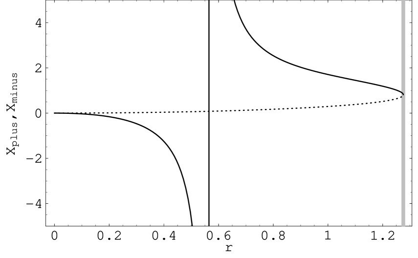
(a) III: $y=0.5$, $a^{2}=4.0$, $e^{2}=1.5$

(b) IVa: $y=0.071$, $a^{2}=0.02$, $e^{2}=1.1$

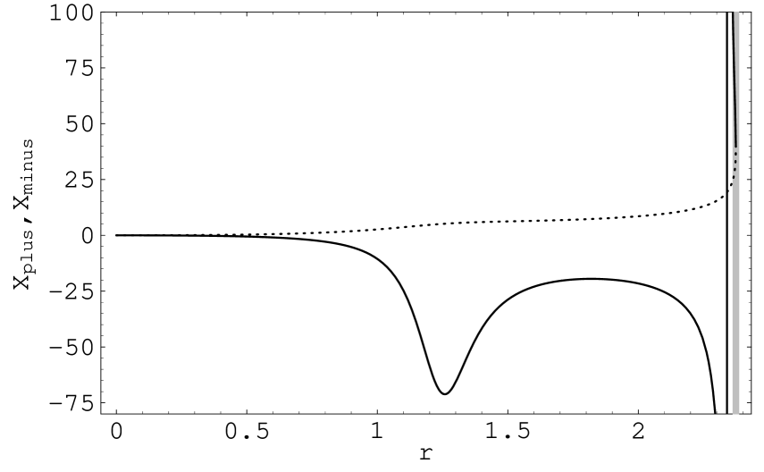
(c) IVb: $y=0.063$, $a^{2}=0.02$, $e^{2}=1.1$

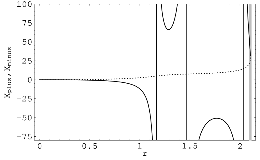
(d) IVc: $y=0.068$, $a^{2}=0.02$, $e^{2}=1.1$

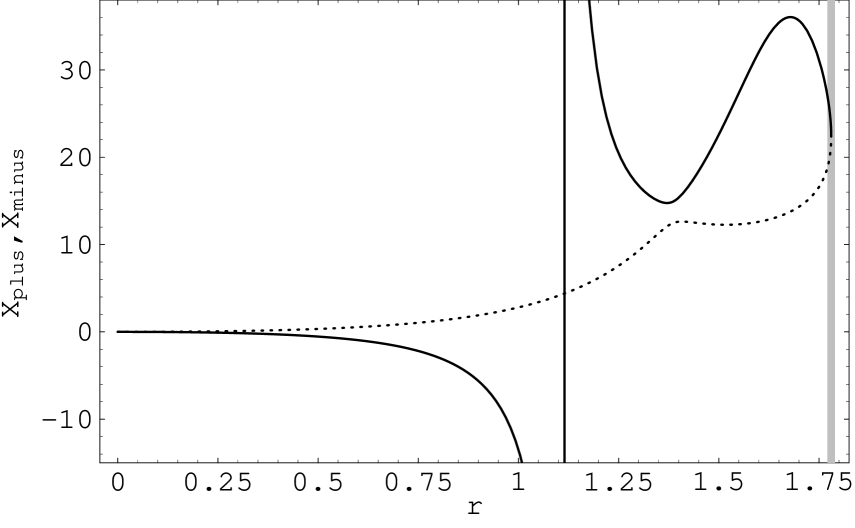
(e) Va: $y=0.0721$, $a^{2}=0.02$, $e^{2}=1.1$

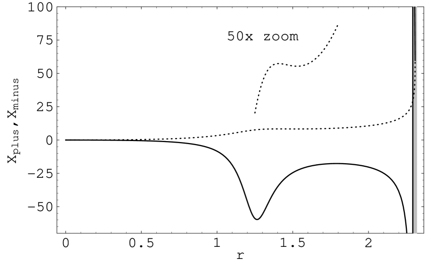
(f) Vb: $y=0.064$, $a^{2}=0.008$, $e^{2}=1.1$

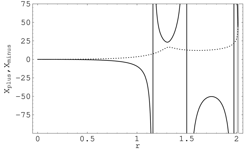
(g) Vc: $y=0.0689$, $a^{2}=0.008$, $e^{2}=1.1$

Figure 9: Typical behavior of effective potential $X_{\pm}$ for Kerr–Newman–de Sitter naked-singularity spacetimes. Stability of the photon circular geodesics can easily be inferred from the character of the effective potential. The vertical bars of the same thickness as the curves are the vertical asymptotes at the points of divergence, the cosmological horizon is depicted as thick gray bar. In order to clearly display the structure of the curves (especially the existence/nonexistence of extremes), certain portions of them are vertically zoomed.

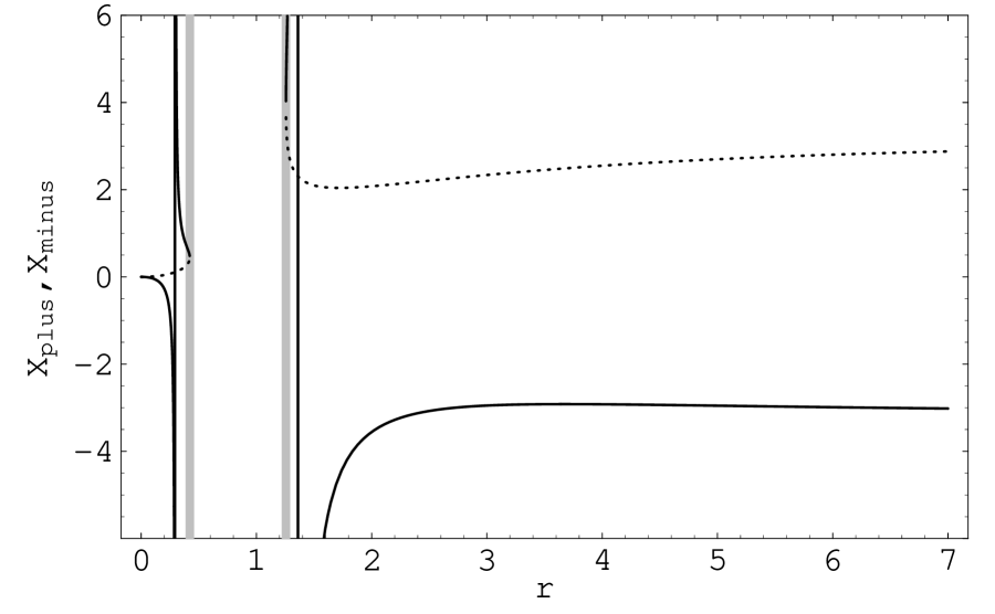
(a) VI: $y=-0.1$, $a^{2}=0.16$, $e^{2}=0.5$

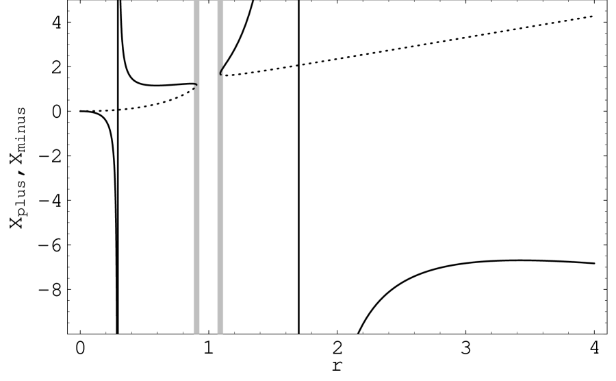
(b) VII: $y=-0.001$, $a^{2}=0.49$, $e^{2}=0.5$

Figure 10: Typical behavior of effective potential $X_{\pm}$ for Kerr–Newman–anti-de Sitter black-holes. Stability of the photon circular geodesics can easily be inferred from the character of the effective potential. The vertical bars of the same thickness as the curves are the vertical asymptotes at the points of divergence, the black-hole horizons are depicted as thick gray bar.

(a) VIII: $y=-0.05$, $a^{2}=0.1$, $e^{2}=1.5$

(b) IXa: $y=-0.01$, $a^{2}=4.0$, $e^{2}=1.5$

(c) IXb: $y=-0.01$, $a^{2}=0.64$, $e^{2}=0.5$

(d) Xa: $y=-0.001$, $a^{2}=0.001$, $e^{2}=1.1$

(e) Xb: $y=-0.014$, $a^{2}=0.06$, $e^{2}=0.95$

Figure 11: Typical behavior of effective potential $X_{\pm}$ for Kerr–Newman–anti-de Sitter naked-singularity spacetimes. Stability of the photon circular geodesics can easily be inferred from the character of the effective potential. The vertical bars of the same thickness as the curves are the vertical asymptotes at the points of divergence. In order to clearly display the structure of the curves (especially the existence/nonexistence of extremes), certain portions of them are vertically zoomed.

Kerr–Newman–de Sitter spacetimes ($y>0$)

Ia:

Black holes with two photon circular orbits and a divergent repulsive barrier between the outer black-hole and cosmological horizons (Fig. 8a). Both circular orbits are unstable relative to radial perturbations.

Ib:

Black holes with two photon circular orbits and a restricted repulsive barrier between the outer black-hole and cosmological horizons (Fig. 8b). Both circular orbits are unstable.

IIa:

Black holes with four photon circular orbits and a divergent repulsive barrier (Fig. 8c). The innermost circular orbit is stable, the others are unstable.

IIb:

Black holes with four photon circular orbits and a restricted repulsive barrier (Fig. 8d). The innermost circular orbit is stable, the others are unstable.

III:

Naked singularities with no circular photon orbit (Fig. 9a).

IVa:

Naked singularities with two circular photon orbits located above the divergent point (Fig. 9b). The inner circular orbit is stable, the outer one is unstable.

IVb:

Naked singularities with two circular photon orbits located under the divergent point (Fig. 9c). The inner circular orbit is stable, the outer one is unstable.

IVc:

Naked singularities with two circular photon orbits and three divergent points (Fig. 9d). The inner circular orbit is stable, the outer one is unstable.

Va:

Naked singularities with four circular photon orbits located above the divergent point (Fig. 9e). Two circular orbits are stable, the others are unstable.

Vb:

Naked singularities with four circular photon orbits located under the divergent point (Fig. 9f). Two circular orbits are stable, the others are unstable.

Vc:

Naked singularities with four circular photon orbits and three divergent points (Fig. 9g). Two circular orbits are stable, the others are unstable.

Kerr–Newman–anti-de Sitter spacetimes ($y<0$)

VI:

Black holes with two photon circular orbits (Fig. 10a). Both circular orbits are unstable.

VII:

Black holes with four photon circular orbits (Fig. 10b). The innermost orbit is stable, the others are unstable.

VIII:

Naked singularities with zero circular photon orbits (Fig. 11a).

IXa:

Naked singularities with two circular photon orbits (Fig. 11b). The inner circular orbit is stable, the outer one is unstable.

IXb:

Naked singularities with two circular photon orbits and two divergent points (Fig. 11c). The inner circular orbit is stable, the outer one is unstable.

Xa:

Naked singularities with four circular photon orbits (Fig. 11d). Two inner orbits are stable, two outer orbits are unstable.

Xb:

Naked singularities with four circular photon orbits and two divergent points (Fig. 11e). Two inner orbits are stable, two outer orbits are unstable.

(a)

(b)

(c)

Figure 12: Parameter space of the Kerr–Newman–de Sitter black-hole spacetimes separated into classes Ia,b and IIa,b. The distribution in the parameter space $y$-$a^{2}$-$e^{2}$ is represented by three qualitatively different $e^{2}={\rm const}$ slices of the space, since the 3D plot with three different surfaces looks rather messy. The typical sections are given for (a) $e^{2}=0.3$, (b) $e^{2}=0.8$, (c) $e^{2}=1.0$. In the cases (b) and (c), the intersection points of $y_{\rm max(ex+)}$ (dotted curve) and $y_{\rm min(h)}$ (full curve crossing the $a^{2}$ axis) are explicitly shown. Dashed curve separates spacetimes with divergent and restricted repulsive barrier.

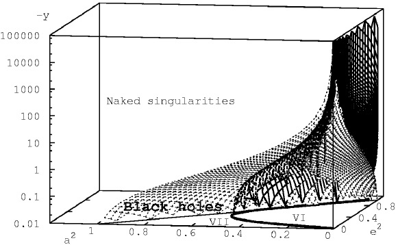
Figure 13: Parameter space of the Kerr–Newman–anti-de Sitter black-hole spacetimes separated into regions corresponding to the class VI and VII in a 3D diagram. We use the logarithmic scale on the $y$-axis because black-hole states are allowed for all negative values of $y$. The light surface ($y_{\rm min(h)}$) separates black-hole and naked-singularity spacetimes, while the dark surface ($y_{\rm max(ex+)}$) separates spacetimes allowing different number of circular photon orbits. Note that the function $y_{\rm max(ex+)}$ diverges for $a^{2}\rightarrow 0$. (For $e^{2}\rightarrow 0$, there is $y_{\rm max(ex+)}(a,e)\rightarrow+\infty$.) The surface $y_{\rm max(ex+)}(a,e)$ intersects the $y=0$ plane at the curve $a^{2}_{\rm ex(z(ex))}(e^{2})$ separating the Kerr–Newman spacetimes with different number of circular photon geodesics (bold curve). The part of the surface $y_{\rm max(ex+)}(a,e)$ at small values of $e^{2}$ is not visualized. It enables to show the intersection of the surfaces $y_{\rm max(ex+)}(a,e)$ and $y_{\rm min(h)}(a,e)$.

Now we determine regions of the parameter space corresponding to the black-hole spacetime classes defined above. Region of the parameter space corresponding to black holes is given in Fig. 12 (classes Ia,b and IIa,b, for spacetimes with a repulsive cosmological constant) and in Fig. 13 (classes VI and VII, for spacetimes with an attractive cosmological constant). For the Kerr–Newman–de Sitter black holes with four photon circular orbits (classes IIa,b), the parameter space is determined by the condition

$$0<y_{\rm min(h)}<y<y_{\rm max(ex+)}<y_{\rm max(h)},$$ (83)

where $y_{\rm max(ex+)}$ corresponds to $y_{\rm ex(ex+)}$, i.e., to the maxima of the function $y_{\rm ex+}(r;a,e)$ taken at $r=\frac{4}{3}e^{2}$. They are determined by the ‘$+$’ branch of the function (64). (Note that the conditions determining black-hole spacetimes with a restricted and divergent repulsive barrier are given by the relation (73), and the distribution of black-hole spacetimes in the parameter space is given completely.) For the Kerr–Newman–anti-de Sitter black holes with four photon circular orbits (class VII), the parameter space is determined by the condition

$$y_{\rm min(h)}<y<y_{\rm max(ex+)}<0,$$ (84)

together with the condition (49) which guarantees that the extremum of $y_{\rm ex+}(r;a,e)$ at $r=\frac{4}{3}e^{2}$ is a maximum. Black holes of class VI (with two photon circular orbits) are determined by the condition

$$y_{\rm max(\rm ex+)}<y<0,$$ (85)

if relation (49) is valid; if $a^{2}<a^{2}_{\rm inf+}(e)$, the spacetimes of class VI are determined by the relation

$$y_{\rm min(h)}<y<0.$$ (86)

For the classes of the naked-singularity spacetimes, the parameter space can be divided into the corresponding separated parts in an analogous manner.

4 Directional angles of photons in black-hole spacetimes with a repulsive cosmological constant

In order to understand the character of the spacetimes with a restricted repulsive barrier, we investigate the behavior of directional angles of equatorial photons as measured by a family of stationary observers in these spacetimes. We determine properties of photon escape/capture cones, and relations between the directional angle of a photon and its impact parameter. It is useful to compare the results with the situation held in the spacetimes with a divergent repulsive barrier, and, especially, with the case of pure Kerr black hole. Because the effects are caused by the rotation parameter of the spacetime, we put $e=0$ for simplicity.

The most convenient family of local stationary observers in the rotating background is the family of locally non-rotating observers, introduced by Bardeen [15]. In the Kerr–de Sitter spacetimes, the tetrad of differential forms corresponding to this family of observers is given by

$$\omega^{(t)}\equiv\left(\frac{\Delta_{r}\Delta_{\theta}\rho^{2}}{I^{2}A}\right)^{1/2}\,{\rm d}t,$$ (87)

$$\omega^{(r)}\equiv\left(\frac{\rho^{2}}{\Delta_{r}}\right)^{1/2}\,{\rm d}r,$$ (88)

$$\omega^{(\theta)}\equiv\left(\frac{\rho^{2}}{\Delta_{\theta}}\right)^{1/2}\ {\rm d}\theta,$$ (89)

$$\omega^{(\phi)}\equiv\frac{A^{1/2}\sin\theta}{I\rho}({\rm d}\phi-\Omega\,{\rm d}t),$$ (90)

where

$$A=(r^{2}+a^{2})^{2}-a^{2}\Delta_{r},$$ (91)

and the angular velocity of such observers

$$\Omega=\Omega(r,\theta;y,a)=\frac{{\rm d}\phi}{{\rm d}t}=\frac{a\left[-\Delta_{r}+(r^{2}+a^{2})\Delta_{\theta}\right]}{A}.$$ (92)

We can convince ourselves easily that both the functions $A$ and $\Omega$ are positive at the stationary regions of the spacetime at $r>0$. For completeness, we present also the tetrad of vectors dual to the differential forms:

$$e_{(t)}=\left(\frac{I^{2}A}{\Delta_{r}\Delta_{\theta}\rho^{2}}\right)^{1/2}\left(\frac{\partial}{\partial t}+\Omega\frac{\partial}{\partial\phi}\right),$$ (93)

$$e_{(r)}=\left(\frac{\Delta_{r}}{\rho^{2}}\right)^{1/2}\frac{\partial}{\partial r},$$ (94)

$$e_{(\theta)}=\left(\frac{\Delta_{\theta}}{\rho^{2}}\right)^{1/2}\frac{\partial}{\partial\theta},$$ (95)

$$e_{(\phi)}=\frac{I\rho}{A^{1/2}\sin\theta}\frac{\partial}{\partial\phi}.$$ (96)

Locally measured components of photon’s 4-momentum $p^{\mu}\equiv{\rm d}x^{\mu}/{\rm d}\lambda$, are given by projections onto the tetrads:

$$p^{(\alpha)}=p^{\mu}\omega^{(\alpha)}_{\mu};\quad p_{(\beta)}=p_{\mu}e^{\mu}_{(\beta)}.$$ (97)

The locally measured components are then related in the simple special-relativistic way,

$$p^{(t)}=-p_{(t)};\quad p^{(\phi)}=p_{(\phi)}.$$ (98)

Now we shall restrict our attention to the equatorial motion of photons. The directional angle $\psi$ of these photons, related to the outward radial direction is generally determined by the relations

$$\sin\psi=\frac{p^{(\phi)}}{p^{(t)}},$$ (99)

$$\cos\psi=\frac{p^{(r)}}{p^{(t)}},$$ (100)

In terms of the impact parameter $X$, the equatorial components of photon’s 4-momentum are given by

$$p^{r}=\frac{{\rm d}r}{{\rm d}\lambda}=\pm\frac{I}{r^{2}}\sqrt{(r^{2}-aX)^{2}-\Delta_{r}X^{2}},$$ (101)

$$p^{\phi}=\frac{{\rm d}\phi}{{\rm d}\lambda}=\frac{I^{2}}{r^{2}}\left[X+\frac{a\left(r^{2}-aX\right)}{\Delta_{r}}\right],$$ (102)

$$p^{t}=\frac{{\rm d}t}{{\rm d}\lambda}=\frac{I^{2}}{r^{2}}\left[aX+\frac{(r^{2}+a^{2})(r^{2}-aX)}{\Delta_{r}}\right],$$ (103)

where the $+(-)$ sign in Eq. (101) corresponds to the outward (inward) photon’s motion. Then we arrive at

$$p^{(r)}=\pm\frac{I}{r\Delta_{r}^{1/2}}\sqrt{(r^{2}-aX)^{2}-\Delta_{r}X^{2}},$$ (104)

$$p^{(\phi)}=\frac{Ir}{A^{1/2}}(X+a),$$ (105)

$$p^{(t)}=\frac{I}{r}\left(\frac{A}{\Delta_{r}}\right)^{1/2}[1-\Omega(X+a)],$$ (106)

and

$$\sin\psi=\frac{r^{2}\Delta_{r}^{1/2}(X+a)}{A[1-\Omega(X+a)]},$$ (107)

$$\cos\psi=\pm\frac{\sqrt{(r^{2}-aX)^{2}-\Delta_{r}X^{2}}}{A^{1/2}[1-\Omega(X+a)]},$$ (108)

or in terms of impact parameter $\ell$, we find the relations

$$\sin\psi=\frac{r^{2}\Delta^{1/2}_{r}\ell}{A(1-\Omega\ell)},$$ (109)

$$\cos\psi=\pm\frac{\sqrt{1-2\Omega\ell+A^{-1}(a^{2}-\Delta_{r})\ell^{2}}}{1-\Omega\ell}.$$ (110)

The angular velocity of the locally non-rotating frames $\Omega(r,\theta=\pi/2;y,a)$ is given by Eq. (92). Now we are able, using the properties of the radial motion, to determine equatorial sections of photon escape (capture, respectively) cones. It is useful to invert the relations (107) and (109), and write

$$X(\psi;r,y,a)=\frac{A(1-a\Omega)\sin\psi-r^{2}a\Delta^{1/2}_{r}}{A\Omega\sin\psi+r^{2}\Delta^{1/2}_{r}},$$ (111)

and

$$\ell(\psi;r,y,a)=\frac{A\sin\psi}{A\Omega\sin\psi+r^{2}\Delta_{r}^{1/2}}.$$ (112)

We can immediately see that, as expected, for the radially directed photons with $\psi=0$, or $\psi=\pi$, the impact parameter $\ell=0$, and $X=-a$.

The function $X(\psi;r,y,a)$ (or $\ell(\psi;r,y,a)$) enables us to determine photon escape (or capture) cones in a straightforward way by using the effective potential $X_{\pm}(r;y,a)$ of the radial motion. The escape cones are given by the directional angles corresponding to the marginally escaping photons having the impact parameters $X_{\rm c}$ corresponding to the unstable circular photon orbits (see Fig. 14).

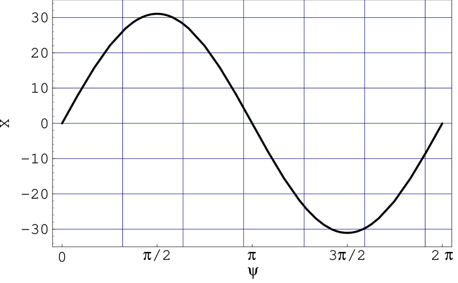
(a)

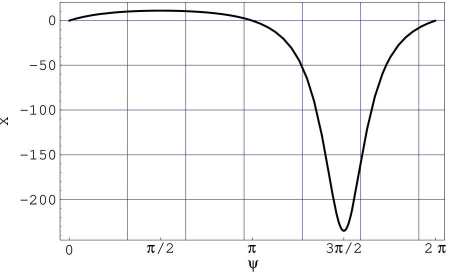
(b)

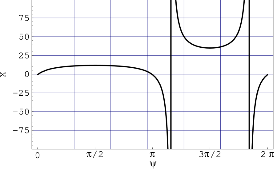
(c)

Figure 14: The dependence of photon’s impact parameter $X(\psi;r,y,a)$ on the directional angle $\psi$ measured relative to the outward direction in the locally non-rotating frames. The dependence is illustrated in three typical cases which are possible in the Kerr–de Sitter black-hole spacetimes. (a) $y=0.036$, $a^{2}=e^{2}=0$, $r=3$ – sinus-like symmetric shape; (b) $y=0.036$, $a^{2}=0.16$, $e^{2}=0$, $r=3$ – the shape is distorted, but the function remains continuous; (c) $y=0.036$, $a^{2}=0.49$, $e^{2}=0$, $r=3.5$ – if the restricted repulsive barrier occurs, discontinuities appear in the function $X(\psi;r,y,a)$.

 

$r=1.44=r_{{\rm h}+,1}+\delta$

$r=1.5$

$r=r_{{\rm min}-,1}$

$r=1.73=r_{{\rm h}+,2}+\delta$

$r=1.75$

 

$r=r_{{\rm min}-,2}$

$r=1.94=r_{{\rm h}+,3}+\delta$

$r=2$

$r=r_{{\rm min}-,3}$

$r=2.2$

 

(Figure continued)

 

$r=2.4$

$r=2.5$

$r=2.7$

$r=r_{{\rm max}+,3}$

$r=3$

 

$r=r_{{\rm max}+,2}$

$r=3.3=r_{{\rm c},3}-\delta$

$r=3.6$

$r=r_{{\rm max}+,1}$

$r=4$

 

(Figure continued)

 

$r=4.2$

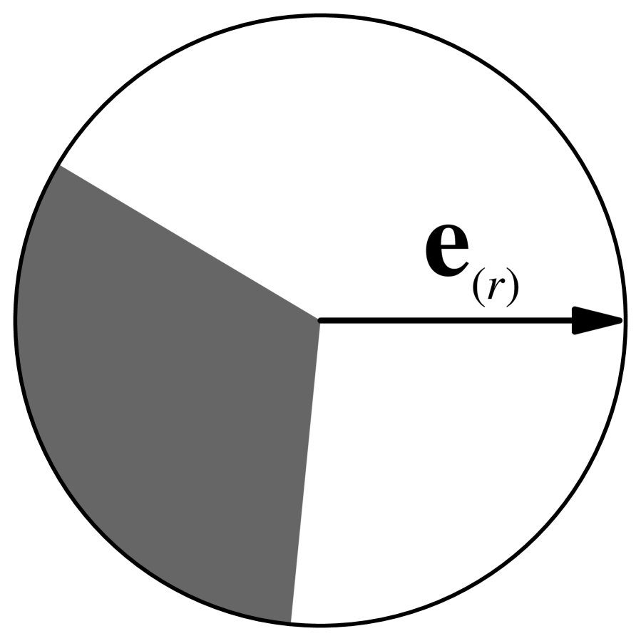
$r=4.29=r_{{\rm c},2}-\delta$

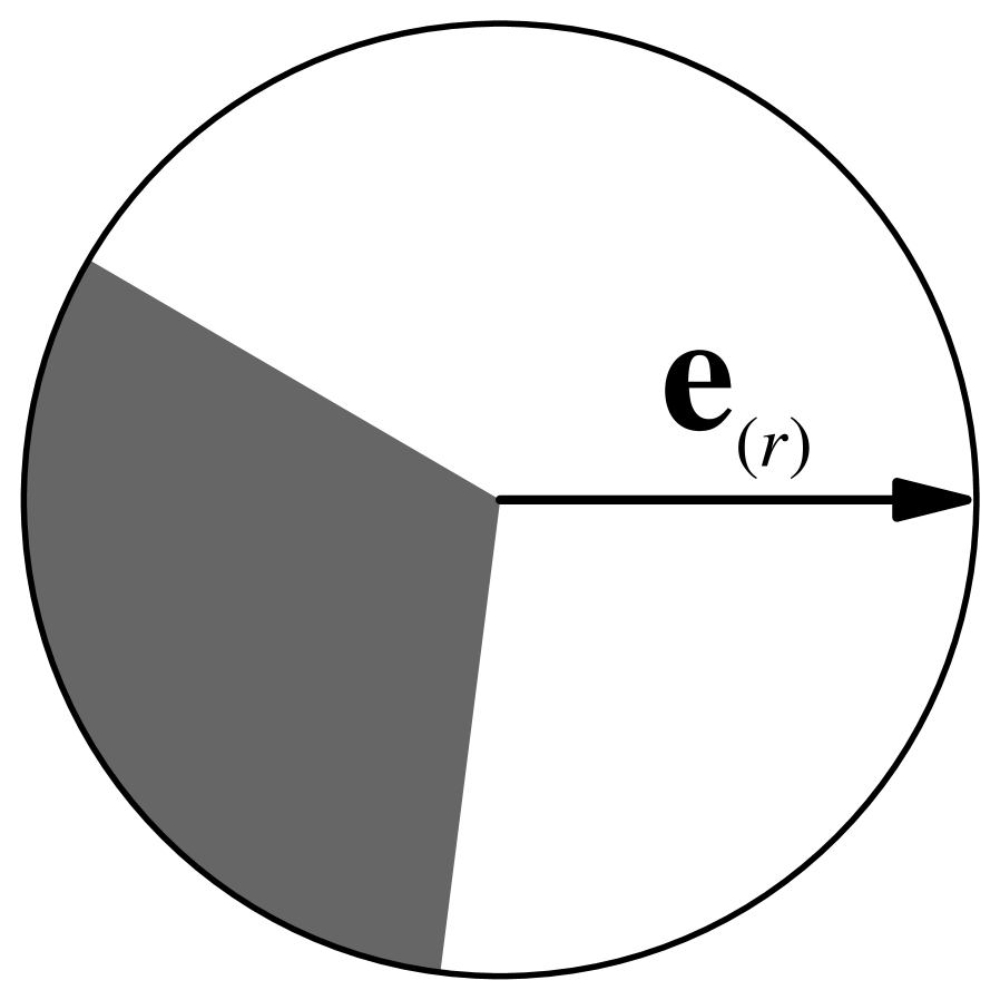
$r=6$

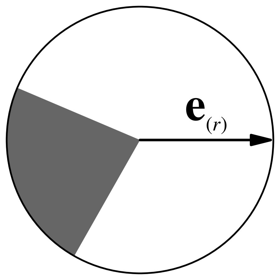
$r=25$

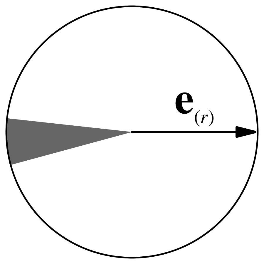
$r=100={}$‘$r_{{\rm c},1}-\delta$’

 

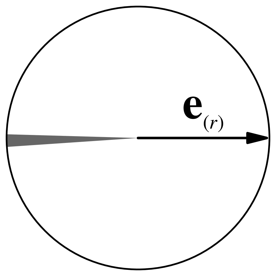
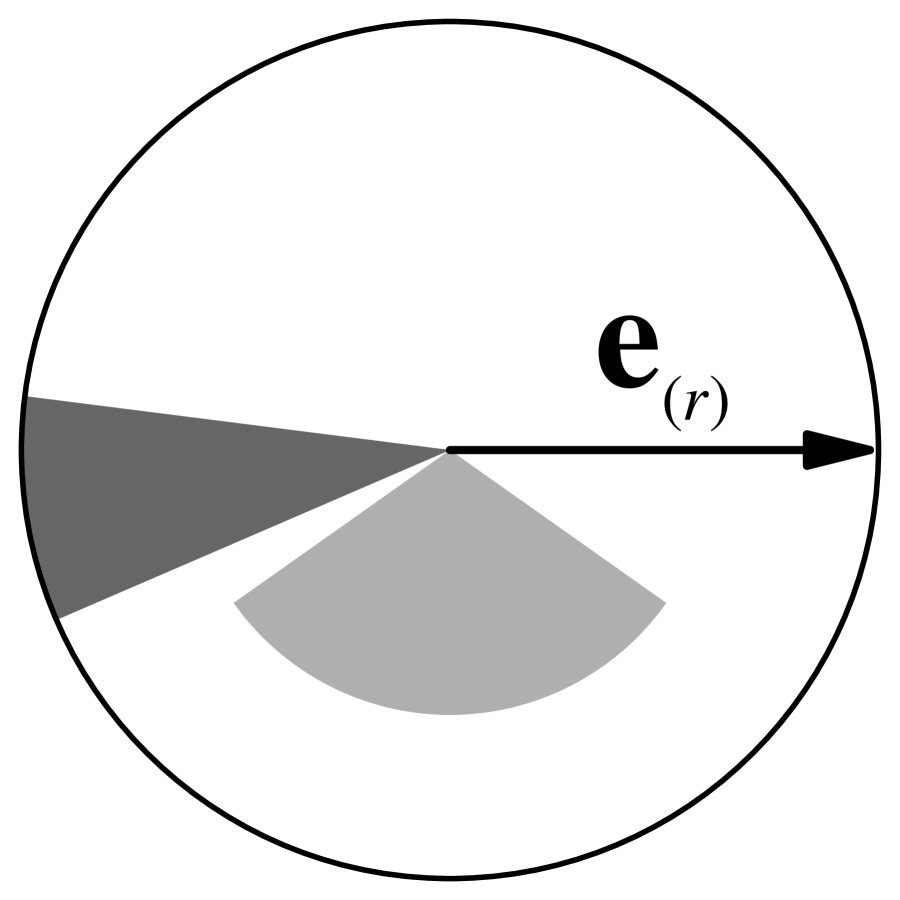
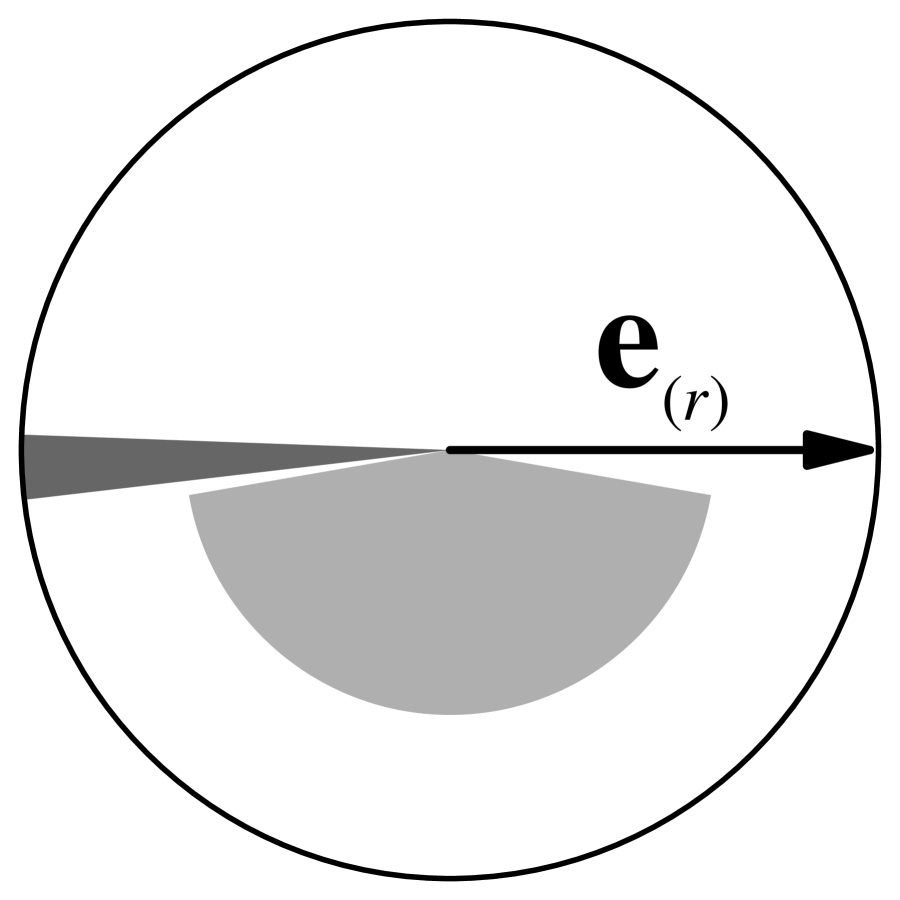
Figure 15: Sectors of captured (dark gray) and escaping (white) equatorial photons for several values of the radius of a LNRF observer for fixed $e^{2}=0$, $a^{2}=0.81$, and (1) $y=0$ (pure Kerr, top rows), (2) $y=0.03$ (Kerr–de Sitter with ‘ordinary’ divergent barrier, middle row), (3) $y=0.04$ (Kerr–de Sitter with restricted repulsive barrier, bottom row, if any). The upper and bottom half-pies correspond to corotating and counterrotating equatorial photons, respectively. Small light gray sectors (if present) mark the interval in which the impact parameter $X(\alpha)$ of the counterrotating equatorial photons is positive. In all the cases above, $\delta$ refers to an appropriately small number. The values of the radii $r_{\rm h+}$ of the outer black-hole horizon, the radii $r_{\rm min-}$ of the local minima of $X_{-}$, the radii $r_{\rm max+}$ of the local maxima of $X_{+}$, and the radii $r_{\rm c}$ of the cosmological horizon, are summarized in Table 1.

In order to understand the nature of the black-hole spacetimes with a restricted repulsive barrier, it is important to notice that there can exist two angles $\psi_{\rm d\pm}$ symmetric with respect to $\psi=3\pi/2$, for which the function $X(\psi;r,y,a)$, or the function $\ell(\psi;r,y,a)$, diverges. The photons counterrotating relative to the locally non-rotating observers at directional angles $\psi\in(\psi_{\rm d-},\psi_{\rm d+})$ have positive impact parameter $X$ (or $\ell$), contrary to the situations we are accustomed to from non-rotating backgrounds. The angles of divergence are determined by the relation

$$\sin\psi_{\rm d\pm}=-\frac{r^{2}\Delta^{1/2}_{r}}{A\Omega}=-\frac{r^{2}\left[(1-yr^{2})(r^{2}+a^{2})-2r\right]^{1/2}}{a\left[yr^{2}(r^{2}+a^{2})+2r\right]}.$$ (113)

Of course, they exist only if the condition $|\sin\psi_{\rm d\pm}|\leq 1$ is satisfied. This condition implies inequality

$$\left[r-2-yr\left(r^{2}+a^{2}\right)\right]\left[r^{3}+a^{2}(r+2)+ya^{2}r\left(r^{2}+a^{2}\right)\right]\leq 0.$$ (114)

However, the condition $X_{+}(r;y,a)>0$ implies the inequality

$$r\left[r-2-yr\left(r^{2}+a^{2}\right)\right]\leq 0.$$ (115)

Table 1: The values of the radii $r_{\rm h+}$ of the outer black-hole horizon, the radii $r_{\rm min-}$ of the local minima of $X_{-}$, the radii $r_{\rm max+}$ of the local maxima of $X_{+}$, and the radii $r_{\rm c}$ of the cosmological horizon (see Fig. 15).

Case	$y$	Outer BH	Radius of the local	Radius of the local	Cosmological
		horizon	minimum of $X_{-}$	maximum of $X_{+}$	horizon
1	0	$r_{{\rm h}+,1}=1.435890$	$r_{{\rm min}-,1}=1.557855$	$r_{{\rm max}+,1}=3.910268$	$r_{{\rm c},1}=\infty$
2	0.03	$r_{{\rm h}+,2}=1.728078$	$r_{{\rm min}-,2}=1.859046$	$r_{{\rm max}+,2}=3.201891$	$r_{{\rm c},2}=4.298185$
3	0.04	$r_{{\rm h}+,3}=1.931337$	$r_{{\rm min}-,3}=2.045904$	$r_{{\rm max}+,3}=2.886223$	$r_{{\rm c},3}=3.302544$

Thus, we can conclude that the angles of divergence occur just at those regions of rotating spacetimes, where the effective potential of the radial photon motion $X_{+}(r;y,a)\geq 0$. Such situation appears in the Kerr spacetimes between the outer horizon and the surface $r=2$. In the Kerr–de Sitter black-hole spacetimes with a divergent repulsive barrier it appears at the vicinity of both the outer black-hole and cosmological horizons, while in the black-hole spacetimes with a restricted repulsive barrier it appear everywhere between the black-hole and cosmological horizons.

In the case of Kerr black-holes the divergent angles are located inside the photon capture cone. For Kerr–de Sitter black holes with a divergent repulsive barrier, the angles of divergence are located inside the photon capture cone in vicinity of the black-hole horizon, while they are located inside the photon escape cone in vicinity of the cosmological horizon. For Kerr–de Sitter black-hole spacetimes with a restricted repulsive barrier, a new phenomenon arises: region between the angles of divergence enters both the escape and capture cones at each radius between the horizons (see Fig. 15).

5 The azimuthal motion

Figure 16: The turning points of the azimuthal equatorial motion of photons. The function $X_{\phi}(r;y,a,e)$ (dashed curve) is drawn along with the effective potential of the radial motion $X_{+}(r;y,a,e)$ (solid curve) and $X_{-}(r;y,a,e)$ (dotted curve). The turning points of the azimuthal motion can appear only in regions where $X_{+}(r;y,a,e)<0$. This example is drawn for $y=0.036$, $a^{2}=0.49$, $e^{2}=0.5$ (class Ia); the horizons are depicted as thick gray bars. The portion below the inner black-hole horizon is vertically zoomed to enable distinguish the curves clearly.

Figure 17: Trajectories of the equatorial photon motion obtained by numerical solving the equations of motion. The two upper rows depict the trajectories in the region between the outer black-hole and cosmological horizons, the bottom row depicts the trajectories in the region beyond the cosmological horizon. The trajectories with both $r$ and $\phi$ monotonously increasing/decreasing are collected in the left column, the trajectories with turning point only in $\phi$ are collected in the middle column, and trajectories with turning points both in $r$ and $\phi$ are collected in the right column (note that there is no such trajectory beyond the cosmological horizon). The values of spacetime parameters are $y=0.036$, $a^{2}=0.49$, $e^{2}=0.5$ (class Ia), the value of impact parameter $X$ and the initial conditions are the following. The two top rows – $X=-10$ (left), $X=-30$ (middle), $X=-50$ (right), the top row has $r_{0}=r_{\rm h+}+\delta$, $\dot{r}_{0}>0$, the middle row has $r_{0}=r_{\rm c}-\delta$, $\dot{r}_{0}<0$. The bottom row – $X=30$ (left), $X=10$ (middle), $r_{0}=r_{\rm c}+\delta$, $\dot{r}_{0}>0$. (Here, $\delta$ refers to an appropriately small number.)

The equation of the azimuthal motion in the equatorial plane can be written in the form

$$\frac{{\rm d}\phi}{{\rm d}\lambda}=\frac{I^{2}}{r^{2}\Delta^{2}}\left[(\Delta_{r}-a^{2})X+ar^{2}\right].$$ (116)

Therefore, turning points of the azimuthal motion (where ${\rm d}\phi/{\rm d}\lambda=0$) are determined by the condition

$$X=X_{\phi}(r;y,a,e)\equiv\frac{ar^{2}}{a^{2}-\Delta_{r}}.$$ (117)

There is only one zero point of $X_{\phi}(r;y,a,e)$, which is located at $r=0$ for any values of parameters $y$, $a$, $e$. Divergences of $X_{\phi}(r;y,a,e)$ are determined by the relation

$$y_{\rm d(\phi)}(r;a,e)\equiv\frac{r^{2}-2r+e^{2}}{r^{2}(r^{2}+a^{2})}\equiv y_{\rm d}(r;a,e).$$ (118)

Therefore, the divergent points of $X_{\phi}(r;y,a,e)$ coincide with the divergent points of $X_{+}(r;y,a,e)$. Since

$$\frac{\partial X_{\phi}}{\partial r}=\frac{2ar}{(a^{2}-\Delta_{r})^{2}}(-yr^{4}+r-e^{2}),$$ (119)

the extrema of $X_{\phi}(r;y,a,e)$ are given by the relation independent of the parameter $a$

$$y=y_{\rm ex(\phi)}(r;e)\equiv\frac{r-e^{2}}{r^{4}}.$$ (120)

We can write

$$X_{\phi}(r;y,a,e)=\frac{a}{a+\sqrt{\Delta r}}X_{+}(r;y,a,e).$$ (121)

Because $a/(a+\sqrt{\Delta r})<1$, we can conclude that

$$X_{\phi}(r;y,a,e)\leq X_{+}(r;y,a,e),$$ (122)

so that the turning points of the azimuthal motion must be located in the regions forbidden by the conditions of the radial motion, if $X_{+}>0$. However, they can exist in the regions where $X_{+}<0$.

We give an example of the behavior of the function $X_{\phi}$ (and function $X_{\pm}$) in the case of the spacetimes of the class Ia in Fig. 16.

By combining the azimuthal equation of motion (116) with the radial one (10), we obtain the equation for trajectories of the equatorial motion in the form

$$\frac{{\rm d}\phi}{{\rm d}r}=\pm\frac{I}{\Delta_{r}}\frac{(\Delta_{r}-a^{2})X+ar^{2}}{\sqrt{(a^{2}-\Delta_{r})X^{2}-2ar^{2}X+r^{4}}};$$ (123)

the $+(-)$ sign corresponds to the outward (inward) motion. The trajectory equation was integrated for typical values of the impact parameter $X$ in the case of spacetimes of the class Ia. (The integral (123) can be expressed in terms of elliptic integrals, but the expressions are too complex.) We illustrate the typical trajectories in Fig. 17; notice the most interesting trajectories with the turning point of the azimuthal motion, which can be both with or without the turning point of the radial motion.

6 Concluding remarks

The analysis of the effective potential of the radial motion of photons in the equatorial plane of the Kerr–Newman spacetimes with a non-zero cosmological constant enables us to separate these spacetimes into eighteen classes according to qualitatively different character of the effective potential reflecting appropriately the properties of the geometry.

From the behavior of the effective potential, one can easily achieve some general conclusions about the equatorial photon motion.

1. In any class of the Kerr–Newman spacetimes with $y\neq 0$ the ring singularity (at $r=0$, $\theta=\pi/2$) can be reached by photons with impact parameter $X=0$ (or $\ell=a$). No other photons can reach the ring singularity.

2. Outside the outer black-hole horizon, two unstable photon circular orbits always exist. Additional two circular photon orbits can exist under the inner horizon, the innermost being stable, the other being unstable. This behavior holds for both asymptotically de Sitter, and anti-de Sitter black holes. Naturally, this property holds also for the Kerr–Newman spacetimes with $y=0$.

3. There can exist naked-singularity spacetimes (with both $y>0$, $y<0$) containing no circular photon orbit.

4. If the naked-singularity spacetimes contain four (or two) circular photon orbits, then two (one) of them are stable, while the others are unstable.

5. In some parts of the field of rotating black holes, there exists an unusual relation between directional angles of equatorial photons as measured by locally non-rotating observers, and their impact parameters. Namely, locally counterrotating photons have positive values of the impact parameter. In the field of Kerr black holes, this phenomenon is limited to vicinity of the black-hole horizon and all such photons must be captured by the black hole. For the Kerr–Newman–de Sitter holes with a divergent repulsive barrier, this phenomenon is limited to vicinity of the black-hole horizon (with all such photons being captured by the hole) and to vicinity of the cosmological horizon (with all such photons escaping through the cosmological horizon). However, for the Kerr–Newman–de Sitter holes with a restricted repulsive barrier, this phenomenon appears at all radii between the black-hole and cosmological horizon, and at all radii such photons are partly captured by the hole and partly escape through the cosmological horizon. Further, the existence of the restricted repulsive barrier is directly related to the fact that photons with positive impact parameter $X$ can be counterrotating relative to the locally non-rotating frames in the complete stationary region between the outer black-hole and cosmological horizons. All photons with positive impact parameter lying above the restricted repulsive barrier are counterrotating in locally non-rotating frames. We probably could expect special optical effects connected with the restricted repulsive barrier of the photon motion.

6. A restricted repulsive barrier exists also for the non-equatorial motion of photons in the Kerr–Newman–de Sitter black hole spacetimes with a restricted repulsive barrier of the equatorial photon motion. One can see it directly, if along with the parameter $X$ a new impact parameter $q$ is introduced in such a way that it disappears for the equatorial motion. The effective potential of the radial motion can then be given in the form [17]

   $$X_{\pm}(r;q,y,a,e)\equiv\frac{ar^{2}\pm\sqrt{\Delta_{r}\left[r^{4}+q(a^{2}-\Delta_{r})\right]}}{a^{2}-\Delta_{r}}.$$ (124)

   Clearly, the properties of divergent points of this function are just the same as for the effective potential of the equatorial photon motion.

   The classification of the Kerr–Newman spacetimes with $y\neq 0$, introduced in the analysis of the equatorial photon motion, can be useful also for the analysis of the non-equatorial photon motion. Particularly, the phenomena of the restricted repulsive barrier is also relevant for the non-equatorial motion.

   A combined discussion of the radial and latitudinal motion enables us to determine photon escape cones of local observers, and, further, to make calculations of various optical phenomena.

7. Turning points of the azimuthal motion can occur only at the region, where the inequality $X_{+}(r;y,a,e)<0$ holds. Trajectories with an azimuthal turning point can also have a radial turning point. Trajectories of photons beyond the cosmological horizon can have a turning point of the azimuthal motion, however, naturally, no turning point of the radial motion.

Acknowlwdgements

This work has been supported by the GAČR Grant No.202/99/0261, by the Committee for Collaboration of Czech Republic with CERN and by the Bergen Computational Physics Laboratory project, an EU Research Infrastructure at the University of Bergen, Norway, supported by the European Community – Access to Research Infrastructure Action of the Improving Human Potential Programme. The authors would like to acknowledge the perfect hospitality and excellent working conditions at the CERN’s Theory Division and the Institute of Physics of the University of Bergen.

References

References

- [1] Krauss L M and Turner M S 1995 Gen. Relativ. Gravit. 27 1137
- [2] Ostriker J P and Steinhart P J 1995 Nature (London) 377 600
- [3] C. S. Kochanek, Astrophys. J. 466, 638 (1996).
- [4] L. M. Krauss, Astrophys. J. 501, 461 (1998).
- [5] G. T. Horowitz and R. C. Myers, ‘The AdS/CFT Correspondence and a New Positive Energy Conjecture for General Relativity’, hep-th/9808079 (1998).
- [6] E. Martinec, ‘Conformal Field Theory, Geometry and Entropy’, hep-th/9809021 (1998).
- [7] A. Sen, ‘Developments in Superstring Theory’, hep-th/9810356v2 (1998).
- [8] Z. Stuchlík and M. Calvani, Gen. Relativ. Gravit. 23, 507 (1991).
- [9] Z. Stuchlík, G. Bao, E. Østgaard, and S. Hledík, Phys. Rev. D 58, 084003 (1998).
- [10] B. Carter, in Black holes, edited by C. De Witt and B. S. De Witt (Gordon and Breach, New York, 1973), p. 57.
- [11] Z. Stuchlík, Bull. Astron. Inst. Czechoslov. 34, 129 (1983).
- [12] Z. Stuchlík, Bull. Astron. Inst. Czechoslov. 32, 366 (1981).
- [13] V. Balek, J. Bičák, and Z. Stuchlík, Bull. Astron. Inst. Czechoslov. 40, 133 (1989).
- [14] J. B. Zel’dovich and I. D. Novikov, Stroenie i evolyutsiya Vselennoj (Nauka, Moscow, 1975).
- [15] J. M. Bardeen, in Black holes, edited by C. De Witt and B. S. De Witt (Gordon and Breach, New York, 1973), p. 215.
- [16] E. W. Kolb and M. S. Turner, The Early Universe, The Advanced Book Progrem, Addison-Wesley Publishing Co., Inc., Redwood City, California, 1990. ISBN 0-201-11603-0.
- [17] Z. Stuchlík and S. Hledík, in preparation.