The effects of a $\kappa$-distribution in the heliosheath on the global heliosphere and ENA flux at 1 AU

Abstract

By the end of 2008 (approximately one year, at the time of writing), the NASA SMall EXplorer (SMEX) mission IBEX (Interstellar Boundary Explorer) will begin to return data on the flux of energetic neutral atoms (ENA’s) observed from an eccentric Earth orbit. This data will provide information about the inner heliosheath (the region of post-shock solar wind) where ENA’s are born through charge-exchange between interstellar neutral atoms and plasma protons. However, the observed flux will be a function of the heliosheath thickness, the shape of the proton distribution function, the bulk plasma flow, and loss mechanisms acting on ENA’s traveling to the detector. As such, ENA fluxes obtained by IBEX can be used to better parametrize global models which can then provide improved quantitative data on the shape and plasma characteristics of the heliosphere. In a recent letter (Heerikhuisen et al., 2007), we explored the relationship between various geometries of the global heliosphere and the corresponding ENA all-sky maps. There we concentrated on energies close to the thermal core of the heliosheath distribution (200 eV), which allowed us to assume a simple Maxwellian profile for heliosheath protons. In this paper we investigate ENA fluxes at higher energies (IBEX detects ENA’s up to 6 keV), by assuming that the heliosheath proton distribution can be approximated by a $\kappa$-distribution. The choice of the $\kappa$ parameter derives from observational data of the solar wind (SW). We will look at all-sky ENA maps within the IBEX energy range, as well as ENA energy spectra in several directions. We find that the use of $\kappa$ gives rise to greatly increased ENA fluxes above 1 keV, while medium energy fluxes are somewhat reduced. We show how IBEX data can be used to estimate the spectral slope in the heliosheath, and that the use of $\kappa$ reduces the differences between ENA maps at different energies. We also investigate the effect introducing a $\kappa$-distribution has on the global interaction between the SW and the local interstellar medium (LISM), and find that there is generally an increase in energy transport from the heliosphere into the LISM, due to the modified profile of ENA’s energies. This results in a termination shock that moves out by 4 AU, a heliopause that moves in by 9 AU and a bow shock 25 AU farther out, in the nose direction.

1 Introduction

With the crossing of the termination shock (TS) by the Voyager 1 and 2 spacecraft (Burlaga et al., 2005; Decker et al., 2005; Stone et al., 2005), the post-shock solar wind (SW) region, known as the inner heliosheath (Zank, 1999), has become an area of increased interest (Heerikhuisen et al., 2006). Despite its non-functioning plasma instrument, Voyager 1 has provided important data on the flow, energetic particle, and magnetic field orientation in the heliosheath, much of which is poorly understood. Now that Voyager 2 has crossed the TS at 84 astronomical units (AU), new data will further increase our understanding of the outer reaches of the heliosphere.

Although in situ measurements by the Voyager spacecrafts are immensely valuable, they do not provide much information about the global structure of the heliosphere-interstellar medium interaction region. The Interstellar Boundary Explorer (IBEX, McComas et al., 2004, 2006) will try to infer global heliospheric structure by surveying the sky in energetic neutral atoms (ENA’s) from Earth orbit. ENA’s are created in the heliosheath after a neutral atom from the local interstellar medium (LISM) charge-exchanges with a plasma proton. The new neutral atom (generally hydrogen) is born from the proton distribution, and, as such, reflects the characteristic plasma conditions at the point of creation. ENA’s propagate virtually ballistically (particularly ENA hydrogen), subject only to the sun’s gravity and radiation pressure. IBEX will directly detect ENA’s and create all-sky maps at a variety of energies between 10 eV and 6 keV at the rate of one complete map every six months.

The challenge to both data analysts and theorists is how to interpret the ENA flux measurements made by the IBEX-Lo (10 eV – 2 keV) and IBEX-Hi (300 eV – 6 keV) instruments. The ENA flux at a given energy will be a function of the properties of the heliosheath along a particular line of sight. As shown in Heerikhuisen et al. (2007), this includes plasma and neutral number densities, plasma flow speed and direction, plasma temperature, and distance to the heliopause (heliosheath thickness). However, that analysis was limited to energies close the thermal core of the heliosheath distribution, since we did not incorporate high energy tails in the ENA parent population due to either pick-up ions, or energetic protons accelerated by other mechanisms.

Recently, Prested et al. (2008) used a $\kappa$-distribution for the ENA parent population to obtain ENA maps. The advantage of using this distribution, as opposed to a Maxwellian, is that it has a power-law tail, and is therefore capable of producing ENA’s at suprathermal energies. However, the focus in that paper was on the IBEX instrument’s response to ENA fluxes, and feed-back of ENA’s on the global solution was not considered.

In this paper we seek to extend the investigations of Heerikhuisen et al. (2007) to higher energies by adopting a $\kappa$-distribution for heliosheath protons, using an approach similar to Prested et al. (2008). The suggestion that the supersonic SW should be described by a $\kappa$-distribution rather than a Maxwellian has a long history (Gosling et al., 1981; Summers & Thorne, 1991). More recently, with the measurement of PUI’s by Ulysses (Gloeckler et al., 2005; Fisk & Gloeckler, 2006), it became apparent that the PUI distribution merged cleanly into the solar wind distribution, yielding an extended energetic tail. This was carried further by Mewaldt et al. (2001) who constructed an extended supersonic SW proton spectrum showing that a high energy tail emerged smoothly from the clearly identifiable low energy solar wind particles. The results of Mewaldt et al. (2001) showed that not only did a continuous power law tail emerge from the thermal distribution, but this tail merged naturally into higher energies associated with (low energy) anomalous cosmic rays (ACR’s) (Decker et al., 2005). The Voyager LECP data obtained in the heliosheath indicates that a power law distribution at thermal energies is maintained, but of course we have no means to show that a tail emerges smoothly from the shocked SW plasma. Nonetheless, we do not expect an abrupt departure from the supersonic SW particle distribution characteristics in that its overall “smoothness” should be preserved.

We use a self-consistently coupled MHD-plasma/kinetic-neutral code to compute a steady-state heliosphere with a $\kappa$-distribution in the SW, and investigate ENA fluxes at 1 AU, looking in particular for signatures which can be related to the heliospheric structure. We begin, however, by investigating the effects of assuming such a distribution on the supersonic and subsonic SW and, due to the non-local coupling mediated by charge-exchanging neutrals, the global heliosphere.

2 The heliosphere with $\kappa$ heliosheath

At around 100 astronomical units (AU) the supersonic SW flow encounters the termination shock (TS), whereupon it becomes subsonic and heated. The hot subsonic SW fills the inner heliosheath and heliotail (these features are visible in the computed plasma distributions shown in Figure 1). At the same time, the solar system is thought to travel supersonically through the partially ionized plasma of the LISM. As a result, a bow shock forms upstream of the heliosphere, and a tangential discontinuity, known as the heliopause (HP), separates the shocked solar and LISM plasmas. Interstellar neutral gas (primarily hydrogen) is weakly coupled to the plasma through charge-exchange, but readily traverses the heliopause (with a filtration ratio of about 45%) and may be detected near Earth at a range of energies that correspond to the creation site of the neutral H, ranging from the LISM to the hot heliosheath, to the fast solar wind.

To determine the flux of neutral atoms at 1 AU, we use a steady-state solution obtained from the 3D heliospheric model based on the 3D MHD code of Pogorelov et al. (2006) and a 3D version of the kinetic neutral hydrogen code of Heerikhuisen et al. (2006). The first self-consistently coupled 3D application of this code appears in Pogorelov et al. (2008). A steady-state is reached by iteratively running the coupled plasma and neutral codes until successive iterations converge. Although several plasma-only models of the heliosphere are still in use, it is now recognized that including neutral atoms in a global model is critical to obtaining the correct location and shape of the termination shock and heliopause, as well as determining the right temperature of the heliosheath, since interstellar neutrals contribute to significant cooling and heating of the inner and outer heliosheath respectively (Pogorelov et al., 2007). We also note that inter-particle collisions do not significantly alter the neutral distribution and that charge-exchange mean free paths are of the order of the size of the heliosphere, so that neutral atoms should ideally be modelled kinetically, with charge-exchange coupling the neutral and charged populations (Baranov & Malama, 1993; Alexashov & Izmodenov, 2005; Heerikhuisen et al., 2006).

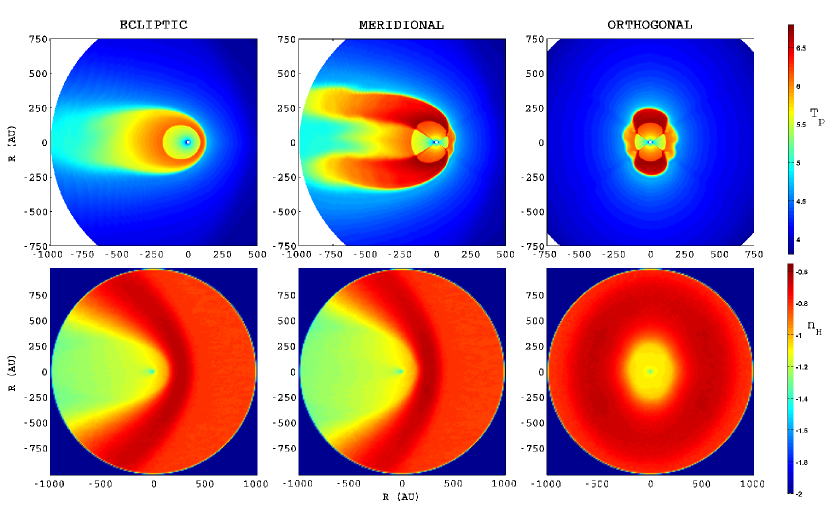
Figure 1: Global heliospheric solution with the boundary conditions described in Table 1. The three columns represent cuts of the heliosphere through the Sun along the ecliptic plane (left), meridional plane (middle), and the plane orthogonal to the LISM flow vector. The top row is a log₁₀ plot of plasma temperature in K, while the bottom row is a log₁₀ plot of neutral density in cm^-3. Distances are in astronomical units (AU). Note how the streams of high speed SW over the poles generate hotter subsonic SW in the heliosheath (Pauls & Zank, 1996, 1997). This high speed wind also symmetrizes the heliopause near the Sun, despite the presence of LISM magnetic field which generally acts to asymmetrize the heliosphere (Pogorelov et al., 2004; Opher et al., 2006), although noticeably less so when neutrals are taken into account (Pogorelov & Zank, 2006; Pogorelov et al., 2007). The build-up of neutral hydrogen just outside the heliopause, known as the “hydrogen wall”, can be clearly seen in the lower plots.

Parameter	Interstellar	1 AU
		Low Speed	High Speed
$U$ (km/s)	26.4	400	800
$T$ (K)	6527	$10^{5}$	2.6$\times 10^{5}$
$n_{p}$ (cm-3)	0.05	7	2.6
$n_{H}$ (cm-3)	0.15	0	0
$|B|$ ($\mu$G)	1.5	37.5 ($B_{r}$)	37.5 ($B_{r}$)
$\phi_{B}$ (∘)	90
$\theta_{B}$ (∘)	60

Table 1: Boundary conditions for the 3D heliospheric model considered here. We use a spherical coordinate system, where $\phi$ is the angle in the ecliptic plane around from the meridional plane and $\theta$ is the angle above the ecliptic plane. The solar rotation axis is assumed orthogonal to the ecliptic plane. The SW is assumed to change from a slow wind to a high speed wind at 35 degrees above the ecliptic plane, as suggested by Ulysses observations (McComas et al., 2000) of the SW during solar minimum.

Our model treats the ion population as a single fluid whose total pressure is the sum of the pressure contribution from electrons, thermal ions (SW or LISM), and PUI’s. Because the pick-up of interstellar neutral H yields a PUI population co-moving with the bulk SW flow, a single fluid model captures exactly the energetics and dynamics of the combined SW/PUI plasma. The only assumption that is needed is for the value of the adiabatic index ($\gamma=2$ corresponds to no scattering of the PUI distribution, $\gamma=5/3$ corresponds to scattering of the PUI’s onto a shell distribution) – see, for example, Khabibrakhmanov et al. (1996) or section 4.1 of Zank (1999). The pick-up of ions and the creation of new H-atoms is included self-consistently through source integrals in the plasma momentum and energy equations (Holzer, 1972; Pauls et al., 1995). The pick-up of interstellar neutrals and the creation of PUI’s in the supersonic SW removes energy and momentum from the SW since the newborn ions are accelerated in the SW motional electric field to co-move with the SW flow. The fast neutrals created in the supersonic SW propagate radially outward, typically experiencing charge-exchange in the LISM. Pick-up of neutrals in the SW therefore decelerates the flow, and since a population of PUI’s with thermal velocities comparable to the bulk SW speed ($\sim 1$ keV energies) is created, the total pressure/temperature in the one-fluid model begins to increase with increasing heliocentric radius. Of course, the thermal SW ions experience no heating other than due to enhanced dissipation associated with excitation of turbulence by the pick-up process (Williams et al., 1995; Zank et al., 1996). These effects are all captured by the self-consistent coupling of plasma, via a one-fluid plasma model, and neutral H, and the plasma pressure and velocity respond directly to the distribution of neutral H throughout the heliosphere. Finally, as neutral H drifts through the heliosphere from the upwind to downwind, neutral H is depleted leading to less pick-up towards the heliotail region. This results in a (relatively weak) upwind-downwind asymmetry in the SW plasma flow velocity (see Figure 2, below) and the one-fluid (i.e. PUI’s) pressure/temperature. It should be noted that these results are independent of the specific form of the plasma ion (thermal and PUI) distribution function, as long as it is assumed isotropic. Only in computing the specific source term for both the plasma and neutral equations does the detailed distribution become important, and then primarily for the neutral distribution (since new-born PUI’s are always accelerated by the motional electric field to co-move with the SW flow).

What we have just described is the heating/pressurization of a single fluid SW due to charge-exchange with interstellar Hydrogen. Our $\kappa$-distribution approach tries to improve on this by using a distribution with core and tail features to approximate the core SW, suprathermal ion, and PUI distributions respectively. Of course in reality the solar wind is much better described by separate distributions. In fact, a drawback of our approach is that the value of $\kappa$ we use fixes the ratio between the core and tail number densities so that one cannot change independently characteristics of the core without making self-similar change to the wings of the $\kappa$-distribution. In particular, this manifests itself in the radial temperature profile of the solar wind. Observations by Richardson et al. (1995) suggest that the core SW does not cool adiabatically, but instead appears to be heated. New-born PUIs form an unstable ring-beam distribution which excites Alfvén waves that then scatter the PUIs onto a bispherical distribution. The power in the excited waves can be computed geometrically as the difference in the energy between the an energy conserving shell distribution for PUIs and a bispherical distribution for PUIs (Williams & Zank, 1994) or directly from quasi-linear theory (Lee & Ip, 1987). To explain the heating observed by Richardson et al. (1995), Williams et al. (1995) suggested that the dissipation of the PUI excited waves could account for the heating, but it was only with the development of a transport model for magnetic field fluctuations and their turbulent dissipation (which leads to heating of the plasma) that the PUI excited fluctuations be properly accounted for (Zank et al., 1996). Since the dissipation of magnetic fluctuation power is strengthened in the outer heliosphere by PUI excited fluctuations, this leads to a corresponding heating of the solar wind plasma in the outer heliosphere. Matthaeus et al. (1999) applied the turbulence transport model of Zank et al. (1996) to show explicitly that PUI enhanced turbulent dissipation of magnetic field fluctuations could account for the observed solar wind plasma heating, a result that was examined in considerably more detail by Smith et al. (2001) (see also Chashei et al., 2003; Smith et al., 2006). The dissipation of magnetic energy affects only the solar wind core, heating it, but leaves the suprathermal and PUI population unchanged energetically. Within a single fluid description, both the core and tail components of the distribution broaden simultaneously, and we cannot alter the ratio of energization between these components, as would be required if we were to account for turbulent dissipation of magnetic fluctuation energy into the solar wind plasma. Nonetheless, the total dynamics of the system, including charge exchange levels, is preserved but the detailed energy allotment between the core SW and PUI’s is fixed by the choice of the $\kappa$ parameter.

Figure 1 shows cuts of the heliosphere in three planes for the plasma temperature and neutral hydrogen density. These results were obtained using our 3D MHD-plasma/kinetic-neutral model, where we assumed a $\kappa$-distribution for protons in the heliosheath with $\kappa=1.63$. The SW and LISM boundary conditions used in this calculation are summarized in Table 1. As described above, the pick-up process for our single ion fluid approach results in solar wind properties expected from observational data – i.e. increased pressure and decreased speed at larger radial distances. To demonstrate this using our code, Figure 2 shows profiles of the bulk speed of the SW, and the fast magnetosonic Mach number given by

$$M=2u_{r}/\left(\sqrt{c_{s}^{2}+\frac{B^{2}}{4\pi\rho}+\frac{|B_{r}|c_{s}}{\sqrt{\pi\rho}}}+\sqrt{c_{s}^{2}+\frac{B^{2}}{4\pi\rho}-\frac{|B_{r}|c_{s}}{\sqrt{\pi\rho}}}\right)\;,$$ (1)

where $\rho$, $P$ and $c_{s}^{2}=\gamma P/\rho$ are the plasma density, pressure and sound speed respectively. The adiabatic index $\gamma=5/3$. The slowdown in our simulation from 400 km/s at 1 AU, down to 335 km/s at the TS matches the 15 % slowdown inferred from Voyager 2 observations (Richardson et al., 2008). Voyager 2 observed a TS compression ratio of about 2 (Richardson, 2007), which corresponds to a Mach number of 1.7 if we assume a simple gas-dynamic shock. Our simulation yields a Mach number of 2.3, which is slightly higher, due, in part, to the absence of a shock precursor. The implications of using a $\kappa$-distribution in the heliosheath, and how this result relates to a traditional Maxwellian approach, is described in the next section.

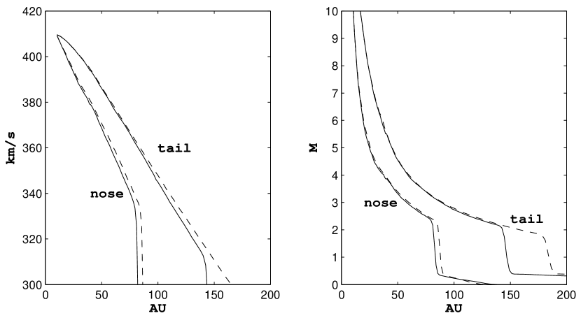
Figure 2: The solar wind bulk speed (left), and the corresponding Mach number as computed from (1). Here we have plotted profiles in both the LISM upwind (nose) and downwind (tail) directions for a model using Maxwellian (solid) and $\kappa$ (dashed) distributions for the solar wind. In our calculation the TS has a Mach number of about 2.3 in the nose direction, and around 2 in the tail. Note also the asymmetry in the solar wind speed from nose to tail, due to the reduced charge-exchange rate in the tail. The SW speed at the inner boundary, located at $r=10$ AU, is slightly higher than indicated in Table 1 due to the thermal acceleration of the SW close to 1 AU.

	Maxwellian	$\kappa=1.63$
TS distance (AU)	83	87
HP distance (AU)	139	131
BS distance (AU)	400	440
$n_{H}$ at TS (cm-3)	0.095	0.09
$n_{H}$ at H-wall (cm-3)	0.23	0.215

Table 2: Comparison of global heliospheric densities and distances in the upstream LISM direction between the solution with a Maxwellian distribution for protons in the heliosheath, and when we take protons to obey a $\kappa$-distribution in the inner heliosheath with $\kappa=1.63$ and allow feed-back of the modified ENA distribution on the global solution.

2.1 Implications of using a $\kappa$-distribution in the heliosheath

Pick-up ions (PUI’s) originate in the SW due to charge-exchange of LISM neutrals with SW protons. However, they do not thermalize with the background SW plasma (Isenberg, 1986; Zank, 1999) and are not therefore equilibrated with the SW. Thus, PUI’s constitute a separate suprathermal population of the SW (Moebius et al., 1985; Gloeckler et al., 1993; Gloeckler, 1996; Gloeckler & Geiss, 1998). PUI’s contribute to the power-law tails observed almost universally in the SW plasma distribution (Mewaldt et al., 2001; Fisk & Gloeckler, 2006). A simple way to add a power-law tail, and thereby model the proton, energetic particle, and PUI populations as a single distribution, is to assume a generalized Lorentzian, or “$\kappa$”, function (Bame et al., 1967; Summers & Thorne, 1991; Collier, 1995; Leubner, 2004) given by

$$f_{p}({\bf v})=\frac{n_{p}}{\pi^{3/2}\Theta_{p}^{3}}\frac{1}{\kappa^{3/2}}\frac{\Gamma(\kappa+1)}{\Gamma(\kappa-1/2)}\left[1+\frac{1}{\kappa}\frac{({\bf v}-{\bf u}_{p})^{2}}{\Theta_{p}^{2}}\right]^{-(\kappa+1)}$$ (2)

where $\Theta_{p}$ is a typical speed related to the effective temperature of the distribution, and is evaluated using the pressure equation (3) below. This distribution has a Maxwellian core, a power-law tail which scales as $v^{-2\kappa-2}$, and reduces to a Maxwellian in the limit of large $\kappa$. Although the core and tail features agree qualitatively with observations, a limitation of the $\kappa$ formalism is that it does not allow us to adjust their relative abundances. The observed flat-topped PUI population is also absent in the $\kappa$ approximation. In Figure 3, we plot a $\kappa$-distribution for $\kappa=1.63$, along with a Maxwellian distribution.

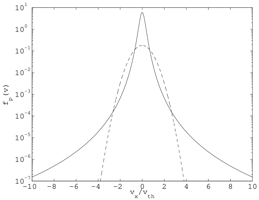
Figure 3: A 1D slice of the velocity distribution function in the plasma frame for $\kappa=1.63$, based on (2) (solid line), along with Maxwellian distribution (dashed). Note that the core of the $\kappa$-distribution is narrower than the Maxwellian. The zeroth and second moments are the same for both distributions. To aid comparison, we have defined $v_{th}=\Theta_{p}\sqrt{\kappa/(\kappa-3/2)}$ to the thermal speed parameter $\Theta_{p}$ of the $\kappa$-distribution, where $v_{th}=2k_{B}T/m_{p}$ is the Maxwellian thermal speed.

The basic principle in our approach is to note that the MHD equations for the plasma do not change if we assume a $\kappa$-distribution for SW protons. This is facilitated by the fact that the basic fluid conservation laws do not assume any specific form of the distribution function (see for example Burgers, 1969). Closure at the second moment is possible if the distribution is isotropic, since the heat flux and the off-diagonal components of the stress tensor are then identically zero. The only difference from conventional fluid dynamics is that the collision integrals do not vanish as they would for a Maxwellian distribution. However, collisional frequencies are so low for the SW that we may neglect these collisional terms and treat the distribution function (2) as “frozen” into the plasma. Even though the SW is effectively collisionless, an MHD approach is still warranted since the plasma has fluid properties perpendicular to the magnetic field, while various wave phenomena help isotropize this (see for example Kulsrud, 1984). For these reasons we solve the regular MHD equations to find the bulk plasma quantities, but in the inner heliosheath we simply interpret these as having come from (2). For simplicity we assume $\kappa=1.63$ in all SW plasma, which is a value consistent with the data analysis of Decker et al. (2005). As we show in Section 4.2, observations by the upcoming IBEX mission can be used to estimate $\kappa$ in the heliosheath.

The two distribution functions, $\kappa$ and Maxwellian, used to model the plasma are linked through the choice of $\Theta_{p}$, and we reconcile these using the isotropic plasma pressure, given by

$$P=\frac{m_{p}}{3}\int_{0}^{\infty}v^{2}f_{p}(v)\;4\pi v^{2}{\rm d}v=\frac{m_{p}n_{p}}{2}\Theta_{p}^{2}\frac{\kappa}{\kappa-3/2}$$ (3)

Note that the thermal core collapses as $\kappa\rightarrow 3/2$ and the pressure becomes undefined. This limiting case corresponds to a $v^{-5}$ tail (Fisk & Gloeckler, 2006). For the purposes of comparison, we define an effective temperature for the $\kappa$-distribution

$$T_{\rm eff}=\frac{P}{n_{p}k_{B}}$$ (4)

The temperature profiles depicted in Figures 1 and 5 refer to the effective temperature.

Charge-exchange couples the neutral and plasma populations. However, the charge exchange loss terms are different when we use a $\kappa$-distribution for protons. In the Appendix we derive the charge exchange rate for a hydrogen atom traveling through a $\kappa$-distribution of protons, which is used in our kinetic code for H atoms in the heliosheath.

Other authors have included pick-up ions into their heliospheric models in various different ways. The Bonn model (Fahr et al., 2000) include PUI’s as a separate fluid with a source term due to interstellar neutrals charge-exchanging in the supersonic SW, and a sink due to PUI’s being energized and becoming part of the anomalous cosmic ray population, which is modeled as a separate fluid. The PUI distribution function of the Bonn model is assumed to be isotropic and flat-topped between 0 and $v_{SW}$ in the frame of the SW. Although this type of distribution agrees reasonably well with observations of PUI’s in the supersonic SW (Gloeckler & Geiss, 1998), the validity of the same distribution downstream of the TS is more questionable. Such a distribution also does not have a tail that extends beyond the pick-up energy, which is a requirement for obtaining ENA’s at high energies. This model was modified in Fahr & Scherer (2004) to include a significant improvement in the form of the PUI distribution, based on the work of Fahr & Lay (2000) which includes analytic estimates of the effects of upstream turbulence. Although restricted by axial symmetry, this model includes time-dependent effects, and allows the authors to estimate various properties of ENA’s.

Malama et al. (2006) recently introduced a more complicated PUI model based on earlier work by Chalov et al. (2003). In this model a host of different neutral atom and PUI populations are tracked kinetically. This model incorporates more physics than our relatively simple $\kappa$-distribution approach, but to manage the added complexity, it also requires a number of additional assumptions. These include the form of the velocity diffusion coefficient, that the magnetic moment is conserved by PUI’s as they cross the TS, and an ad hoc assumption about the downstream energy partition between electrons, protons and PUI’s. The increased computational requirements also forces Malama et al. (2006) to consider only the case of axial symmetry, thereby neglecting the IMF and restricting the ISMF to being aligned with the flow. Although their assumptions are reasonable, it is difficult to determine the influence these have on their conclusions. One of the interesting results from their model is that the locations of the TS, HP and BS change when the effects of PUI’s are allowed to self-consistently react back on the plasma – a result which agrees quite well quantitatively with our findings in the next section.

3 Effects of heliosheath $\kappa$-distribution on the global solution

In the preceding section we showed that we may solve the regular MHD equations for the plasma in the heliosheath, and interpret these results in terms of a $\kappa$-distribution for the ion population. It is less clear, however, what the effects of $\kappa$-distributed neutral atoms originating from the heliosheath will have on the global heliosphere-interstellar medium solution. Figure 4 shows the velocity distribution of heliosheath hydrogen at various locations along the LISM flow vector. It is clear from this figure that for a $\kappa=1.63$ distribution significantly more H-atoms with energies above 1 keV result than for a Maxwellian ion population in the heliosheath. It is also important to note that ENA’s in the heliotail (left plot) show a clear power-law tail ($\sim v^{-2(\kappa+1)}$), mirroring the plasma, when a $\kappa$-distribution is assumed for heliosheath protons. These tails persist even outside the heliosphere (middle and right plots) for energies above 1 keV.

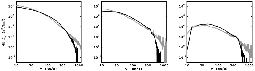
Figure 4: Velocity distributions of ENA’s at three locations along the axis defined by the LISM flow vector with the Sun at the origin: -400 AU in the heliotail (left), 180 AU upstream in the hydrogen wall (middle), 600 AU in the nearby LISM (right). The black line is for ENA’s obtained from a Maxwellian distribution of heliosheath ions (the parent population of ENA’s), while the gray line is commensurate to a $\kappa=1.63$ distribution for heliosheath protons in the same steady-state configuration. Note that for small $\kappa$ we have less medium energy ENA’s, but more at low and high energies, in agreement with the respective distributions shown in Figure 3.

To test the effect of keV ENA’s on the global heliosphere, we ran our code with $\kappa=1.63$ in the heliosheath, and allowed these ENA’s to feed back self-consistently on the global solution. Since H-atoms are modeled kinetically, this provides no extra difficulty for our model. The only difference, by comparison with the case of a Maxwellian proton distribution, is that we need to use a different formula for the relative motion between a given particle and the ambient plasma. This formula is derived in the appendix.

Figure 5 compares plasma density and temperature along radial lines in the nose, polar and tail directions for the Maxwellian and equilibrated $\kappa=1.63$ heliosheath cases. Secondary charge-exchange of neutrals created in the hot heliosheath was identified by Zank et al. (1996) as a critical medium for the anomalous transport of energy from the shocked solar wind to the shocked and unshocked LISM. In particular, the upwind region abutting the HP experienced considerable heating as a result of secondary charge-exchange of hot ($\sim 10^{6}$ K) neutrals with the cold LISM protons. The efficiency of this medium of anomalous heat transfer is increased with a $\kappa$-distribution in the inner heliosheath. This results simultaneously in a shrinking of the inner heliosheath and an expansion of the outer heliosheath. The inner heliosheath plasma temperature (defined in terms of pressure) remains unchanged, because the Maxwellian and $\kappa$-distributions have the same second moment (see Section 2.1). We find that in the nose direction the termination shock moves out by about 4 AU, while the heliopause moves inward by about 9 AU. The bow shock stand-off distance increases by 25 AU, and the shock itself is weakened by the additional heating of the LISM plasma by fast neutrals from the SW. Table 2 summarizes these changes in heliospheric geometry. The observed modifications to the heliospheric discontinuity locations agree quite well with the changes observed by the multi-component heliospheric model of Malama et al. (2006), which includes a kinetic representation of PUI’s. These authors report a 5 AU increase in the TS distance and a 12 AU decrease in the distance to the HP, for an axially symmetric calculation without magnetic fields.

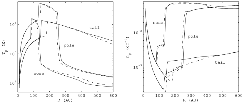
Figure 5: Radial profiles of effective plasma temperature (left) and density (right) in the nose, polar (i.e. in the meridional plane), and tail directions. The solid line represents the values obtained by using a Maxwellian distribution function for the proton distribution and ENA’s generated from it. The dashed line is obtained by assuming that the proton distribution in the supersonic and subsonic SW can be described as an isotropic $\kappa$-distribution with $\kappa=1.63$. Although the MHD equations do not change in the latter case, the distribution function of ENA’s born through charge-exchange in the heliosheath becomes more $\kappa$-like (see Figure 4) and their secondary charge-exchange outside the heliosheath alters the global plasma configuration. The temperature plots also demonstrate the relationship between PUI pressure and SW speed, with the fast SW over the poles showing a much higher temperature/pressure than the slower ecliptic SW.

Another important distinction between the Maxwellian and $\kappa$-distribution based models is that the filtration rate of hydrogen changes at the heliopause. We find that in the Maxwellian case the hydrogen density at the TS is about 63% of the interstellar value, while for the $\kappa$-distributed model the density drops slightly to 60%. As with the TS and HP locations, these results agree quite well with the Malama et al. (2006) model.

4 Implications for IBEX

The Interstellar Boundary EXplorer mission will provide all-sky maps of ENA’s coming from the inner heliosheath, at 14 energy bands from 10 eV to 6 keV. However, this data is unusual in that all the ENA’s detected at a particular pixel and energy bin, will have come from a large volume of space with non-uniform plasma properties. As such it is not possible to invert an ENA map to determine the heliosheath’s shape, size, and plasma distribution. For this reason, we need to use forward modeling to help us understand the relationship between model heliosheaths and their corresponding synthetic ENA maps. In Heerikhuisen et al. (2007), we identified several possible signatures to infer heliosheath properties from IBEX data. Below we present ENA maps and spectra from our improved heliospheric model, and relate these to the properties of our model heliosheath.

4.1 Ionization losses

ENA’s propagating from the heliosheath to a detector at 1 AU may experience re-ionization due to charge exchange, electron impact ionization, or photo-ionization. These effects are of major importance close to the Sun, and in the simplest approximation scale according to

$$w=w_{0}\exp(-\int\beta\;{\rm d}t)\;,\quad\beta(r)=\beta_{E}/r^{2}[AU]\;,\quad\beta_{E}\simeq 6\times 10^{-7}{\rm s}^{-1}$$ (5)

where $w$ is a pseudo-particle weight which is initially equal to $w_{0}$ at the point of charge-exchange and decays with time as a function of position. Alternatively, we can view $w/w_{0}$ as the survival probability for a particular particle. We note here that $\beta_{E}$ does not have to be uniform in all directions, so that ionization losses for particles coming in over the poles could be different from those traveling in the ecliptic plane, and it may also have temporal variations.

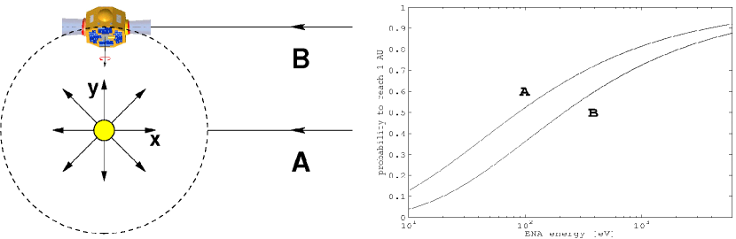
Figure 6: Schematic (left) showing the difference between ENA flux at 1 AU (dashed circle) along path A, and the ENA flux IBEX will measure along path B. Note that the IBEX instrument always points perpendicular to the radial vector from the Sun. The right plot shows the different survival probabilities along the two paths from some point in the heliosheath (effectively infinity) to 1 AU, due to charge-exchange, electron impact and photo-ionization losses.

Generally ENA’s will travel on effectively straight trajectories since solar gravity is approximately balanced by radiation pressure. Bzowski & Tarnopolski (2006) show that for solar minimum conditions the deflection angle will be less than 5 degrees, even for the lowest energies we consider. In the simulations presented here, we assume zero deflection, since we are mainly interested in the gross features of the ENA maps. Trajectory “A” in Figure 6 shows the shortest straight-line path to 1 AU for an ENA, while path B represents the longest. If we assume straight line propagation at constant speed $-v_{0}$, then the survival probability (i.e. $w/w_{0}$) is given by

$$P=\exp\left(-\frac{\beta_{E}}{v_{0}}\int_{1}^{\infty}\frac{1}{x^{2}+y_{0}^{2}}{\rm d}x\right)\;,$$

where $y_{0}=0$ for path A and $y_{0}=1$ for path B. Upon integration we have

$$P_{A}=\exp\left(-\frac{\beta_{E}}{v_{0}}\right)\;,\quad P_{B}=\exp\left(-\frac{\pi\beta_{E}}{2v_{0}}\right)$$ (6)

where $v_{0}$ is the particle speed in AU per second. Here path B is relevant to IBEX observations, but experiences more ionization losses. A simple $\pi/2$ factor can be used to switch between 1 AU fluxes and IBEX fluxes, assuming no deflection due to gravity or radiation pressure occurs. Figure 6 shows survival probability profiles for both paths, and we note that profile “A” corresponds to Figure 4 of Gruntman et al. (2001). These loss formulae will we used in the next section to undo the losses simulated in the code so that we can use the pristine ENA fluxes to construct energy spectra. Such a procedure would also be necessary for IBEX data, when we want to infer properties of the parent plasma.

4.2 ENA spectra

We may extract information about the proton energy spectrum in the heliosheath by simply plotting the IBEX energy bin data for a particular pixel (i.e. direction). Our global model allows us to both prescribe a form for the distribution function in the heliosheath for ENA’s (i.e. $\kappa$) and then attempt to deconvolve this from the data. The only difference is that IBEX spectral data will be line-of-sight integrated, rather than at a particular point in space. Nevertheless, we have the global data from our model, which we can use to compare an IBEX line-of-sight spectrum with plasma properties along that line of sight. This is particularly interesting in the nose direction, where the plasma distribution observed by the Voyager spacecraft can be compared with the spectral slope inferred from the IBEX data.

To obtain a more accurate representation of the ENA spectrum in the heliosheath, we need to undo the ionization losses experienced by particles as they travel to the detector. In Section 4.1 we derived a simple expression to estimate the survival probability of a particle with a given energy along a particular line of sight. Figure 7 shows three energy spectra for ENA’s originating from the nose, tail and polar directions. For these spectra, we have divided the flux measured at 1 AU by the survival probability for each energy band to undo the ionization losses, as mentioned above. We find that for the three directions considered, the energy spectrum tends toward the value of $-\kappa$ above about 1 keV. This result shows that the IBEX data, in spite of being line-of-sight integrated, should be able to help determine the spectral slope of the heliosheath protons in the 0.6 – 6 keV range.

Figure 7 also shows that the spectra in the three directions considered have very similar properties. This will not necessarily be true for the real heliosphere, where the post-shock SW may develop different high energy tails in different directions. The dotted line (labeled “nose2”) is for a spectrum in the nose direction obtained using 32 energy bins (compared to about 10 non-overlapping IBEX bins). The agreement between this curve and the green markers shows that, for $\kappa=1.63$ at least, the number of IBEX bins is sufficient to reproduce the spectrum.

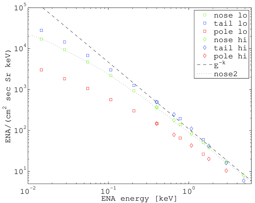
Figure 7: ENA energy spectra as observed at 1 AU along various lines of sight. Here the squares and diamonds represent data using approximate IBEX energy bins obtained by dividing the IBEX-lo and IBEX-hi energy ranges (0.01 – 2.0 keV and 0.3 – 6 keV) into 8 and 6 equal bins on a logarithmic scale respectively (see also Prested et al., 2008). The dotted line was obtained using narrower bins (32 total), and demonstrates that the IBEX bin widths are sufficiently narrow to maintain accuracy. The dashed line has a slope of $-\kappa$, which represents the plasma spectrum at a particular point, and appears reasonably well reproduced along the lines of sight considered.

4.3 ENA all-sky maps

The method we use for computing all-sky ENA maps is described in Heerikhuisen et al. (2007), where we first obtain a steady-state heliosphere and then trace ENA’s born through charge-exchange in the heliosheath down to 1 AU, where these are then binned according to energy and the direction of origin. Additional ionization losses along the particle’s trajectory act to “evaporate” its computational weight. The key difference from our previous results is that we now assume a $\kappa$-distribution for the heliosheath protons which form the parent population for ENA’s. This modification allows us to obtain ENA’s up to several keV, and is more consistent with SW data.

Figure 8 shows all-sky ENA maps obtained from our steady-state solution with a $\kappa$-distribution for heliosheath protons. The top right plot shows the ENA map for 200 eV, which can be compared with our previous work (Heerikhuisen et al., 2007), where we did not self-consistently couple the plasma and kinetic neutral atoms, and where we assumed a Maxwellian proton distribution. We find that when we use a $\kappa$-distribution, the ENA flux at 200 eV is two to three times smaller than for the Maxwellian case, due to the shape of the proton distribution (see Figure 3) and resulting ENA distribution (Figure 4), as well as the thinner inner heliosheath resulting from the use of a $\kappa$-distribution (see Section 3). As expected, this decrease of medium energy (100’s of eV) ENA’s is compensated by an increased ENA flux above 1 keV. Our results predict a count rate of about 3 atoms per (cm² sr s keV) at 6 keV.

Less obvious is the decline in low energy flux when compared to the Maxwellian results (Heerikhuisen et al., 2007), even though there are more ENA’s being generated at the lowest energies (see Figure 4). The principal reason for this is that the SW core temperature is significantly lower when we use $\kappa$, so that these ENA’s lack the energy to propagate upstream, since the bulk speed exceeds the thermal speed of the core. This low SW core temperature is in fact qualitatively consistent with the latest Voyager 2 findings (Richardson, 2007).

The heliosphere depicted in Figure 1, is commensurate to approximately “solar minimum” conditions, with a clearly defined high speed wind emanating from the poles. The high speed wind gives rise to hotter high latitude heliosheath plasma, which in turn increases the energy of ENA’s generated in the subsonic polar SW. The all-sky maps of Figure 8 show that at energies above about 1 keV, these streams of hot SW dominate the ENA flux, while at lower energies the central tail region is the major source of ENA’s.

Comparing skymaps at different energies, we see from Figure 8 that the qualitative properties do not vary widely over the IBEX energy range. This contrasts sharply with the results for a Maxwellian heliosheath, where we generally see a higher flux coming from the tail than the nose at low energies, and the reverse at high energies (Heerikhuisen et al., 2007). This can be attributed to the steep decline in the Maxwellian distribution, compared to the much broader $\kappa$-distribution (see Figure 3), which means that particles observed at a given energy have come from plasma with a narrower range of temperatures. In other words, the relatively cool plasma in the distant heliotail can still be a significant source of high energy ENA’s, if we assume it has a $\kappa$-distribution. Only at the highest energies, above about 2 keV, does the nose-tail asymmetry favor the nose direction.

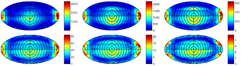
Figure 8: All-sky maps of energetic neutral atom flux at 1 AU, in units of (cm² sr s keV)^-1, generated in the inner heliosheath through charge-exchange between an interstellar neutral atom and a heliosheath proton drawn from a $\kappa$-distribution with $\kappa=1.63$. The direction of the LISM flow is at the center of the plot, with the poles top and bottom, and the heliotail on the far sides. Contour lines have been drawn at 15 degrees intervals. Maps are generated by binning ENA’s which intersect the 1 AU sphere on radially inward trajectories. The maps shown are for the following energies and bin-widths (in eV): $10\pm 2$, $50\pm 10$, $200\pm 20$, $1000\pm 100$, $2400\pm 200$, and $6000\pm 400$ (from top left to bottom right).

5 Conclusions

We have used our 3D MHD-kinetic code to investigate the impact of assuming an alternative heliosheath proton distribution, a $\kappa$-distribution rather than the more usual Maxwellian, on both the SW-LISM interaction region, and the observed ENA flux at 1 AU. The motivation for this is that pick-up ions, generated when an interstellar neutral atom charge-exchanges in the supersonic solar wind, form high energy tails that are always observed in the solar wind plasma. The $\kappa$-distribution has core and tail features, and is often invoked in data analysis of the SW proton distribution function. The use of a $\kappa$-distribution introduces (possibly) more realistic estimates of the ENA flux at 1 AU, and thereby serves as an important tool in reconciling global heliospheric models with data from the upcoming IBEX mission. One drawback of this approach is that we cannot control the ratio between core and tail populations. While obviously not capturing the full details of the thermal and PUI plasma distributions in either the inner heliosheath or throughout the supersonic SW, a $\kappa$-distribution is nonetheless well grounded in observations as a general representation of the SW distribution function.

We used $\kappa=1.63$ in our calculations, based on the Voyager 1 LECP data of Decker et al. (2005). Although the LECP data is for much higher energies than IBEX will measure, we have shown that IBEX data can be used to infer the spectral slope of the heliosheath distribution for energies between 1 keV and 6 keV. The tails of the energy spectra may have different slopes in different directions (over the poles, for example).

The use of a $\kappa$-distribution for the ENA parent proton population results in a significant increase of the ENA flux at energies above 1 keV, when compared with a Maxwellian distribution. Our results predict a count rate of about 3 per (cm² sr s keV) at the highest energies considered by IBEX, which is many orders of magnitude higher than could be expected from a Maxwellian heliosheath distribution. At the same time, there is a marked reduction in the flux for intermediate energies, to about half the Maxwellian value at a few hundred eV. We have also calculated the feed back of the revised ENA distribution on the global heliospheric solution. The result is an increased transport of energy from the inner to the outer heliosheath, with a corresponding thinning and expansion of the former and latter. The distance between the TS and HP decreases by 13 AU (about 25%) in the nose direction, and the bow shock moves out farther and becomes very weak. The thinner heliosheath is also partly responsible for the decreased ENA flux at energies of a few hundred eV.

Finally, we note that we have not considered time-dependent effects in this paper. Sternal et al. (2007) recently looked at the changes in the ENA maps when they included a simple model for the solar cycle into their 3D hydrodynamic (i.e. no magnetic fields) code which includes a single fluid for neutral gas. They found cyclic changes in the ENA flux at 100 eV, which varied by about 25%. The observed variations at 1 keV were considerably larger, but because they assumed a Maxwellian distribution for protons in the heliosheath, their fluxes were about an order of magnitude lower than ours at this energy. Effectively, they found that fluctuations in ENA flux due to the solar cycle are relatively small for energies close to the core of the distribution (a few hundred eV in the heliosheath), while at high energies the changes in ENA flux are larger. Since the $\kappa$-distribution declines much more slowly than the Maxwellian away from the core, we expect our ENA fluxes to vary by perhaps 50% over a solar cycle for energies relevant to IBEX. This, however, remains to be confirmed.

Appendix: Charge-exchange formulation with a $\kappa$- distribution

Our kinetic neutral atom method solves the time-dependent Boltzmann equation

$$\frac{\partial}{\partial t}f_{H}+{\bf v}\cdot\nabla f_{H}+\frac{\bf F}{m_{p}}\nabla_{\bf v}\cdot f_{H}=P-L\;,$$ (7)

using a Monte Carlo approach. Here $f_{H}$ is the distribution function of neutral hydrogen, ${\bf F}$ is the external force, and $P$ and $L$ are the production and loss terms. Below we derive the loss rate for a neutral particle traveling through a $\kappa$-distribution of protons.

The production and loss rates for the hydrogen population may be written as

$$P=f_{p}({\bf x},{\bf v},t)\eta({\bf x},{\bf v},t)\;,$$ (8)

$$L=f_{H}({\bf x},{\bf v},t)\beta({\bf x},{\bf v},t)\;,$$ (9)

where

$$\eta({\bf x},{\bf v},t)=\int\sigma_{ex}f_{H}({\bf x},{\bf v}_{H},t)\;|{\bf v}-{\bf v}_{H}|\;{\rm d}{\bf v}_{H}$$ (10)

$$\beta({\bf x},{\bf v},t)=\int\sigma_{ex}f_{p}({\bf x},{\bf v}_{p},t)\;|{\bf v}-{\bf v}_{p}|\;{\rm d}{\bf v}_{p}\;.$$ (11)

Here we assume that the charge exchange cross-section, approximated using the Fite et al. (1962) expression

$$\sigma_{ex}(v_{rel})=\left[2.1-0.092\ln(v_{rel})\right]^{2}10^{-14}{\rm cm}^{2}\;,$$ (12)

varies slowly and can be taken outside the integrals in (10) and(11).

In the kinetic code we require the neutral loss term $\beta$ to compute charge-exchange on a particle-by-particle basis. To derive this, we use the $\kappa$-distribution for the charged component, i.e.,

$$f_{p}({\bf v}_{p})=\frac{n_{p}}{\pi^{3/2}\Theta_{p}^{3}}\frac{1}{\kappa^{3/2}}\frac{\Gamma(\kappa+1)}{\Gamma(\kappa-1/2)}\left[1+\frac{1}{\kappa}\frac{({\bf v}_{p}-{\bf u}_{p})^{2}}{\Theta_{p}^{2}}\right]^{-(\kappa+1)},$$ (13)

where ${\bf u}_{p}$ is the bulk speed and $\Theta_{p}$ is related to the plasma pressure via equation (3).

Upon introduction of the new variables ${\bf g}=({\bf v}-{\bf v}_{p})/(\sqrt{\kappa}\Theta_{p})$ and ${\bf x}=({\bf u}_{p}-{\bf v}_{p})/(\sqrt{\kappa}\Theta_{p})$, equation (11) becomes

$$\beta=\frac{n_{p}\sigma_{ex}\Theta_{p}}{\pi^{3/2}}\frac{\sqrt{\kappa}\Gamma(\kappa+1)}{\Gamma(\kappa-1/2)}\int g[1+({\bf g}-{\bf x})^{2}]^{-(\kappa+1)}d^{3}g$$

$$=\frac{2n_{p}\sigma_{ex}\Theta_{p}}{\sqrt{\pi}}\frac{\sqrt{\kappa}\Gamma(\kappa+1)}{\Gamma(\kappa-1/2)}\int_{0}^{\infty}dg\int_{-1}^{1}d\mu\;g^{3}(1+g^{2}-2\mu gx+x^{2})^{-(\kappa+1)},$$ (14)

where $\mu=\cos\theta$, $\theta$ being the angle between ${\bf g}$ and ${\bf x}$. After integrating over $\mu$ the result is

$$\beta=\frac{n_{p}\sigma_{ex}\Theta_{p}}{\sqrt{\pi\kappa}x}\frac{\Gamma(\kappa+1)}{\Gamma(\kappa-1/2)}\int_{0}^{\infty}g^{2}\left\{[1+(g-x)^{2}]^{-\kappa}-[1+(g+x)^{2}]^{-\kappa}\right\}dg.$$ (15)

Introducing the new variable $z=g-x$ in the first term and $z=g+x$ in the second term and using the symmetry properties of the integrand, we obtain

$$\beta=\frac{2n_{p}\sigma_{ex}\Theta_{p}}{\sqrt{\pi\kappa}x}\frac{\Gamma(\kappa+1)}{\Gamma(\kappa-1/2)}\left(\int_{0}^{x}z^{2}(1+z^{2})^{-\kappa}dz+x^{2}\int_{0}^{x}(1+z^{2})^{-\kappa}dz\right.$$

$$\left.+2x\int_{x}^{\infty}z(1+z^{2})^{-\kappa}dz\right).$$ (16)

The integrals are

$$x^{2}\int_{0}^{x}(1+z^{2})^{-\kappa}dz=x^{3}\,{{}_{2}F}_{1}\left(\frac{1}{2},\kappa;\frac{3}{2};-x^{2}\right)=x^{3}(1+x^{2})^{-\kappa}\,{{}_{2}F}_{1}\left(1,\kappa;\frac{3}{2};\frac{x^{2}}{1+x^{2}}\right),$$ (17)

$$2x\int_{x}^{\infty}z(1+z^{2})^{-\kappa}dz=\frac{x(1+x^{2})^{-k+1}}{(k-1)},$$ (18)

$$\int_{0}^{x}z^{2}(1+z^{2})^{-\kappa}dz=\frac{x^{3}}{3}\,{{}_{2}F}_{1}\left(\frac{3}{2},\kappa;\frac{5}{2};-x^{2}\right)=\frac{x^{3}}{3}(1+x^{2})^{-\kappa}\,{{}_{2}F}_{1}\left(1,\kappa;\frac{5}{2};\frac{x^{2}}{1+x^{2}}\right),$$ (19)

where ${}_{2}F_{1}$ is the hypergeometric function. The exact solution for $\beta$ is therefore

$$\beta=\frac{2n_{p}\sigma_{ex}\Theta_{p}}{\sqrt{\pi\kappa}}\frac{\Gamma(\kappa+1)}{\Gamma(\kappa-1/2)}(1+x^{2})^{-\kappa}\left[x^{2}\,{{}_{2}F}_{1}\left(1,\kappa;\frac{3}{2};\frac{x^{2}}{1+x^{2}}\right)\right.$$

$$\left.+\frac{x^{2}}{3}\,{{}_{2}F}_{1}\left(1,\kappa;\frac{5}{2};\frac{x^{2}}{1+x^{2}}\right)+\frac{1+x^{2}}{\kappa-1}\right].$$ (20)

However, it is more convenient to take the limits $\sqrt{\kappa}x\ll 1$ and $\sqrt{\kappa}x\gg 1$ in (17) and (19) before the integration. In the former limit we obtain

$$x^{2}\int_{0}^{x}(1+z^{2})^{-\kappa}dz\simeq x^{3},$$ (21)

$$\int_{0}^{x}z^{2}(1+z^{2})^{-\kappa}dz\simeq\frac{x^{3}}{3}$$ (22)

and the expression inside the parentheses in (Appendix: Charge-exchange formulation with a $\kappa$- distribution) becomes $x/(\kappa-1)+x^{3}/3$. Finally, in this limit

$$\beta=\frac{2n_{p}\sigma_{ex}\Theta_{p}}{\sqrt{\pi\kappa}}\frac{\Gamma(\kappa+1)}{\Gamma(\kappa-1/2)}\left[\frac{1}{\kappa-1}+\frac{({\bf v}_{p}-{\bf u}_{p})^{2}}{3\kappa\Theta_{p}^{2}}\right].$$ (23)

For large $\kappa$, $\Gamma(\kappa+a)\simeq\kappa^{a}\Gamma(\kappa)$ and

$$\beta\simeq\frac{2n_{p}\sigma_{ex}\Theta_{p}}{\sqrt{\pi}}\left[1+\frac{({\bf v}-{\bf u}_{p})^{2}}{3\Theta_{p}^{2}}\right].$$ (24)

In the limit $x\gg 1$ we obtain

$$x^{2}\int_{0}^{\infty}(1+z^{2})^{-\kappa}dz=\frac{\sqrt{\pi}\Gamma(\kappa-1/2)x^{2}}{2\Gamma(\kappa)},$$ (25)

$$\int_{0}^{\infty}z^{2}(1+z^{2})^{-\kappa}dz=\frac{\sqrt{\pi}\Gamma(\kappa-3/2)}{4\Gamma(\kappa)}.$$ (26)

In this limit

$$\beta\simeq n_{p}\sigma_{ex}|{\bf v}-{\bf u}_{p}|$$ (27)

and is independent of $\kappa$. A reasonable approximation to (Appendix: Charge-exchange formulation with a $\kappa$- distribution) that has the correct asymptotic behavior is

$$\beta\simeq n_{p}\sigma_{ex}\sqrt{\frac{4\Gamma^{2}(\kappa+1)\Theta_{p}^{2}}{\pi\kappa(\kappa-1)^{2}\Gamma^{2}(\kappa-1/2)}+({\bf v}-{\bf u}_{p})^{2}}.$$ (28)

For large $\kappa$ this reduces to the Maxwellian limit obtained by Pauls et al. (1995)

$$\beta\simeq n_{p}\sigma_{ex}\sqrt{\frac{4}{\pi}\Theta_{p}^{2}+({\bf v}-{\bf u}_{p})^{2}}.$$ (29)

References

- Alexashov & Izmodenov (2005) Alexashov, D., & Izmodenov, V. 2005, Astron. Astrophys., 439, 1171
- Bame et al. (1967) Bame, S. J., Asbridge, J. R., Felthauser, H. E., Hones, E. W., & Strong, I. B. 1967, J. Geophys. Res., 72, 113
- Baranov & Malama (1993) Baranov, V.B., & Malama, Yu. G. 1993, J. Geophys. Res., 98, 15157
- Burgers (1969) Burgers, J. M. 1969, Flow Equations for Composite Gases (Flow Equations for Composite Gases, New York: Academic Press, 1969)
- Burlaga et al. (2005) Burlaga, L. F., Ness, N. F., Acuña, M. H., Lepping, R. P., Connerney, J. E. P., Stone, E. C., & McDonald, F. B. 2005, Science, 309, 2027
- Bzowski & Tarnopolski (2006) Bzowski, M., & Tarnopolski, S. 2006, in American Institute of Physics Conference Series, Vol. 858, Physics of the Inner Heliosheath, ed. J. Heerikhuisen, V. Florinski, G. P. Zank, & N. V. Pogorelov, 251
- Chalov et al. (2003) Chalov, S. V., Fahr, H. J., & Izmodenov, V. V. 2003, J. Geophys. Res., 108, 1266
- Chashei et al. (2003) Chashei, I. V., Fahr, H. J., & Lay, G. 2003, Annales Geophysicae, 21, 1405
- Collier (1995) Collier, M. R. 1995, Geophys. Res. Lett., 22, 2673
- Decker et al. (2005) Decker, R. B., Krimigis, S. M., Roelof, E. C., Hill, M. E., Armstrong, T. P., Gloeckler, G., Hamilton, D. C., & Lanzerotti, L. J. 2005, Science, 309, 2020
- Fahr et al. (2000) Fahr, H. J., Kausch, T., & Scherer, H. 2000, Astron. Astrophys., 357, 268
- Fahr & Lay (2000) Fahr, H. J., & Lay, G. 2000, Astron. Astrophys., 356, 327
- Fahr & Scherer (2004) Fahr, H.-J., & Scherer, K. 2004, Astrophys. Space Sci. Trans., 1, 3
- Fisk & Gloeckler (2006) Fisk, L. A., & Gloeckler, G. 2006, ApJ, 640, L79
- Fite et al. (1962) Fite, W.L., Smith, A. C. H., & Stebbings, R. F. 1962, Proc. R. Soc. London Ser. A, 268, 527
- Gloeckler (1996) Gloeckler, G. 1996, Space Science Reviews, 78, 335
- Gloeckler et al. (2005) Gloeckler, G., Fisk, L. A., & Lanzerotti, L. J. 2005, in ESA Special Publication, Vol. 592, ESA Special Publication
- Gloeckler & Geiss (1998) Gloeckler, G., & Geiss, J. 1998, Space Science Reviews, 86, 127
- Gloeckler et al. (1993) Gloeckler, G., et al. 1993, Science, 261, 70
- Gosling et al. (1981) Gosling, J. T., Asbridge, J. R., Bame, S. J., Feldman, W. C., Zwickl, R. D., Paschmann, G., Sckopke, N., & Hynds, R. J. 1981, J. Geophys. Res., 86, 547
- Gruntman et al. (2001) Gruntman, M., Roelof, E. C., Mitchell, D. G., Fahr, H. J., Funsten, H. O., & McComas, D. J. 2001, J. Geophys. Res., 106, 15767
- Heerikhuisen et al. (2006) Heerikhuisen, J., Florinski, V., & Zank, G. P. 2006, J. Geophys. Res., 111, A06110
- Heerikhuisen et al. (2006) Heerikhuisen, J., Florinski, V., Zank, G. P., & Pogorelov, N. V.(editors). 2006, Physics of the Inner Heliosheath (AIP)
- Heerikhuisen et al. (2007) Heerikhuisen, J., Pogorelov, N. V., Zank, G. P., & Florinski, V. 2007, ApJ, 655, L53
- Holzer (1972) Holzer, T. E. 1972, J. Geophys. Res., 77, 5407
- Isenberg (1986) Isenberg, P. A. 1986, J. Geophys. Res., 91, 9965
- Khabibrakhmanov et al. (1996) Khabibrakhmanov, I. K., Summers, D., Zank, G. P., & Pauls, H. L. 1996, ApJ, 469, 921
- Kulsrud (1984) Kulsrud, R. M. 1984, in Basic Plasma Physics: Selected Chapters, Handbook of Plasma Physics, Volume 1, ed. A. A. Galeev & R. N. Sudan, 115
- Lee & Ip (1987) Lee, M. A., & Ip, W.-H. 1987, J. Geophys. Res., 92, 11041
- Leubner (2004) Leubner, M. P. 2004, Physics of Plasmas, 11, 1308
- Malama et al. (2006) Malama, Y. G., Izmodenov, V. V., & Chalov, S. V. 2006, A&A, 445, 693
- Matthaeus et al. (1999) Matthaeus, W. H., Zank, G. P., Smith, C. W., & Oughton, S. 1999, Physical Review Letters, 82, 3444
- McComas et al. (2006) McComas, D., et al. 2006, in Physics of the Inner Heliosheath, ed. J. Heerikhuisen, V. Florinski, G. P. Zank, & N. V. Pogorelov, Vol. 858 (AIP), 400
- McComas et al. (2004) McComas, D., et al. 2004, in Physics of the Outer Heliosphere, ed. V. Florinski, N. V. Pogorelov, & G. P. Zank, Vol. 719 (AIP), 162
- McComas et al. (2000) McComas, D. J., et al. 2000, J. Geophys. Res., 105, 10419
- Mewaldt et al. (2001) Mewaldt, R. A., et al. 2001, in American Institute of Physics Conference Series, Vol. 598, Joint SOHO/ACE workshop ”Solar and Galactic Composition”, ed. R. F. Wimmer-Schweingruber, 165
- Moebius et al. (1985) Moebius, E., Hovestadt, D., Klecker, B., Scholer, M., & Gloeckler, G. 1985, Nature, 318, 426
- Opher et al. (2006) Opher, M., Stone, E. C., & Liewer, P. C. 2006, Astrophys. J., 640, L71
- Pauls & Zank (1996) Pauls, H. L., & Zank, G. P. 1996, J. Geophys. Res., 101, 17081
- Pauls & Zank (1997) Pauls, H. L., & Zank, G. P. 1997, J. Geophys. Res., 102, 19779
- Pauls et al. (1995) Pauls, H. L., Zank, G. P., & Williams, L. L. 1995, J. Geophys. Res., 100, 21,595
- Pogorelov et al. (2008) Pogorelov, N. V., Heerikhuisen, J., & Zank. 2008, ApJ, 675, in press
- Pogorelov et al. (2007) Pogorelov, N. V., Stone, E. C., Florinski, V., & Zank, G. P. 2007, ApJ, 668, 611
- Pogorelov & Zank (2006) Pogorelov, N. V., & Zank, G. P. 2006, in Astronomical Society of the Pacific Conference Series, Vol. 359, Numerical Modeling of Space Plasma Flows, ed. G. P. Zank & N. V. Pogorelov, 184
- Pogorelov et al. (2004) Pogorelov, N. V., Zank, G. P., & Ogino, T. 2004, Astrophys. J., 614, 1007
- Pogorelov et al. (2006) Pogorelov, N. V., Zank, G. P., & Ogino, T. 2006, Astrophys. J., 644, 1299
- Prested et al. (2008) Prested, C., et al. 2008, J. Geophys. Res., accepted
- Richardson (2007) Richardson, J. D. 2007, AGU Fall Meeting Abstracts, A3
- Richardson et al. (2008) Richardson, J. D., Liu, Y., & Wang, C. 2008, Advances in Space Research, 41, 237
- Richardson et al. (1995) Richardson, J. D., Paularena, K. I., Lazarus, A. J., & Belcher, J. W. 1995, Geophys. Res. Lett., 22, 325
- Smith et al. (2006) Smith, C. W., Isenberg, P. A., Matthaeus, W. H., & Richardson, J. D. 2006, ApJ, 638, 508
- Smith et al. (2001) Smith, C. W., Matthaeus, W. H., Zank, G. P., Ness, N. F., Oughton, S., & Richardson, J. D. 2001, J. Geophys. Res., 106, 8253
- Sternal et al. (2007) Sternal, O., Fichtner, H., & Scherer, K. 2007, Astron. Astrophys., to appear
- Stone et al. (2005) Stone, E. C., Cummings, A. C., McDonald, F. B., Heikkila, B. C., Lal, N., & Webber, W. R. 2005, Science, 309, 2017
- Summers & Thorne (1991) Summers, D., & Thorne, R. M. 1991, Physics of Fluids B, 3, 1835
- Williams & Zank (1994) Williams, L. L., & Zank, G. P. 1994, J. Geophys. Res., 99, 19229
- Williams et al. (1995) Williams, L. L., Zank, G. P., & Matthaeus, W. H. 1995, J. Geophys. Res., 100, 17059
- Zank (1999) Zank, G. P. 1999, Space Sci. Rev., 89, 413
- Zank et al. (1996) Zank, G. P., Matthaeus, W. H., & Smith, C. W. 1996, J. Geophys. Res., 101, 17093
- Zank et al. (1996) Zank, G. P., Pauls, H. L., Williams, L.L., & Hall, D.T. 1996, J. Geophys. Res., 101, 21639