Simulating full-sky interferometric observations

Abstract

Aperture array interferometers, such as that proposed for the Square Kilometre Array (SKA), will see the entire sky, hence the standard approach to simulating visibilities will not be applicable since it relies on a tangent plane approximation that is valid only for small fields of view. We derive interferometric formulations in real, spherical harmonic and wavelet space that include contributions over the entire sky and do not rely on any tangent plane approximations. A fast wavelet method is developed to simulate the visibilities observed by an interferometer in the full-sky setting. Computing visibilities using the fast wavelet method adapts to the sparse representation of the primary beam and sky intensity in the wavelet basis. Consequently, the fast wavelet method exhibits superior computational complexity to the real and spherical harmonic space methods and may be performed at substantially lower computational cost, while introducing only negligible error to simulated visibilities. Low-resolution interferometric observations are simulated using all of the methods to compare their performance, demonstrating that the fast wavelet method is approximately three times faster that the other methods for these low-resolution simulations. The computational burden of the real and spherical harmonic space methods renders these techniques computationally infeasible for higher resolution simulations. High-resolution interferometric observations are simulated using the fast wavelet method only, demonstrating and validating the application of this method to realistic simulations. The fast wavelet method is estimated to provide a greater than ten-fold reduction in execution time compared to the other methods for these high-resolution simulations.

1 Introduction

The next generation of interferometers, such as the Square Kilometre Array (SKA), will have to overcome a number of challenging imaging issues. Key among these is the question of how to deal with very large fields of view, both in terms of the forward problem of simulating observed visibilities and also in terms of the reverse problem of reconstructing wide field images. The reverse wide field imaging problem has been tackled traditionally by faceting the sky into a number of regions which are sufficiently small that the standard tangent plane approximation to Fourier imaging is possible (Cornwell & Perley, 1992; Greisen, 2002). More recently, Cornwell et al. (2005) have introduced the $w$-projection algorithm, providing an order of magnitude speed improvement over facet-based approaches. The forward wide field imaging problem is an issue which arises when observing with interferometric aperture arrays, such as those proposed for the low frequency instrument of the SKA, and which has yet to be resolved.

The final configuration and system design of the SKA are still under active development. The final design will be dependent on the result of simulations. Such simulations are created specifically to assess different array configurations, whilst taking into account a range of sky models and possible error contributions. These simulations are not only important in determining the response of the interferometer to the real sky but also in establishing the dynamic range of an observation when faced with bright sources in the sidelobes of the primary beam. As a consequence, simulating the response of an aperture array interferometer correctly is as vital to the design studies of such instruments as it is important for devising an effective method of reducing the data when they finally arrive.

Such simulations are relatively simple for interferometers with small fields of view. Small fields can be well approximated as planes tangent to the celestial sphere. This approximation allows the visibilities observed by an interferometer to be related to the tangent plane image through the Fourier transform. It is then straightforward to simulate visibilities and reconstruct images. In the case of aperture arrays, which may see the entire hemisphere, the operation is not so trivial. A tangent plane approximation is obviously inappropriate for such geometries and hence the Fourier transform can no longer be used to simulate observed visibilities.

In this article we relax the small field of view assumption and tackle interferometry when considering contributions over the entire sky. We derive full-sky interferometry formalisms using a number of different representations, including representations in real, spherical harmonic and wavelet spaces, and discuss the relative merits of each approach. Other authors have considered the spherical harmonic representation of the interferometry integral relating the intensity of the sky to the visibilities observed by an interferometer, predominantly in the context of observations of the cosmic microwave background (CMB). White et al. (1999) relate the visibilities of observations of the CMB to cosmological quantities of interest, such as the angular power spectrum, through contact with the spherical harmonics. However, the flat tangent plane approximation is still made and hence these results remain restricted to small fields of view. Bunn & White (2007) extend the work of White et al. (1999) to larger fields of view by using mosaicing, making the flat-sky approximation for each individual pointing used to construct the mosaic. Ng (2001) was the first to present the spherical harmonic representation of the interferometry integral while including full-sky contributions, also in the context of computing the angular power spectrum of observations of the CMB. Ng (2001) goes on to discuss implications of this result on properties of the angular power spectrum recovered from interferometric observations. In a separate piece of work, Ng (2005) discusses the recovered full-sky power spectra of CMB experiments with asymmetric window functions. Although all of these works do address spherical harmonic representations of interferometry, and in some cases include contributions over the entire sky, the prevailing context of these works is implications for the angular power spectrum recovered from observations of the CMB. Relatively little attention has been paid to full-sky interferometry formulations in the context of forward or inverse wide field imaging, which pose important problems for next generation interferometers. The purpose of this article is to address these issues, focusing particularly on the forward wide field imaging problem.

The remainder of this article is organised as follows. In Sec. 2 we present the mathematical foundations underlying results derived later in this paper, including a discussion of harmonic analysis, wavelets and rotations on the sphere. In Sec. 3 we derive representations of the interferometric visibility integral in real, spherical harmonic and wavelet space, while including full-sky contributions. The implications of these results for forward and inverse wide field imaging are discussed. In Sec. 4 we present resolution simulations of full-sky interferometric observations using all of the methods discussed in Sec. 3. Concluding remarks are made in Sec. 5.

2 Mathematical preliminaries

Before presenting the formulation of interferometry on the full sky, it is necessary to outline some mathematical preliminaries. We review harmonic analysis and wavelets on the two-sphere ${\mathrm{S}^{2}}$, before discussing rotations, which are represented by elements of the rotation group ${\mathrm{SO}(3)}$. By making all assumptions and definitions explicit we hope to avoid any confusion over the conventions adopted.

2.1 Spherical harmonics

We consider the space of square integrable functions $\mathrm{L}^{2}({\mathrm{S}^{2}},\mathrm{\,d}\Omega)$ on the unit two-sphere ${\mathrm{S}^{2}}$, where $\mathrm{\,d}\Omega(\mbox{\boldmath${\hat{s}}$})=\sin\theta\mathrm{\,d}\theta\mathrm{\,d}\varphi$ is the usual rotation invariant measure on the sphere and $(\theta,\varphi)$ denote the spherical coordinates of $\mbox{\boldmath${\hat{s}}$}\in{\mathrm{S}^{2}}$, with colatitude $\theta\in[0,\pi]$ and longitude $\varphi\in[0,2\pi)$. A square integrable function on the sphere $F\in\mathrm{L}^{2}({\mathrm{S}^{2}},\mathrm{\,d}\Omega)$ may be represented by the spherical harmonic expansion

$$F(\mbox{\boldmath${\hat{s}}$})=\sum_{\ell=0}^{\infty}\sum_{m=-\ell}^{\ell}{F}_{{\ell}{m}}Y_{\ell m}({\mbox{\boldmath${\hat{s}}$}})\>,$$

where the spherical harmonic coefficients are given by the usual projection onto the spherical harmonic basis functions through the inner product:

$${F}_{{\ell}{m}}=\int_{{\mathrm{S}^{2}}}F(\mbox{\boldmath${\hat{s}}$})\>Y_{\ell m}^{\ast}({\mbox{\boldmath${\hat{s}}$}})\mathrm{\,d}\Omega(\mbox{\boldmath${\hat{s}}$})\>.$$

The $\ast$ denotes complex conjugation. We adopt the Condon-Shortley phase convention where the normalised spherical harmonics are defined by (Varshalovich et al., 1989)

$$Y_{\ell m}({\mbox{\boldmath${\hat{s}}$}})=(-1)^{m}\sqrt{\frac{2\ell+1}{4\pi}\frac{(\ell-m)!}{(\ell+m)!}}\>P_{\ell}^{m}({\cos\theta})\>{\rm e}^{{\rm i}m\varphi}\>,$$

where $P_{\ell}^{m}({x})$ are the associated Legendre functions. Using this normalisation the orthogonality of the spherical harmonic functions reads

$$\int_{\mathrm{S}^{2}}Y_{\ell m}({\mbox{\boldmath${\hat{s}}$}})\>Y_{\ell^{\prime}m^{\prime}}^{\ast}({\mbox{\boldmath${\hat{s}}$}})\mathrm{\,d}\Omega(\mbox{\boldmath${\hat{s}}$})=\delta_{{\ell}{\ell^{\prime}}}\delta_{{m}{m^{\prime}}}\>,$$

where $\delta_{ij}$ is the Kronecker delta function.

We complete this section by noting two identities of which we will make subsequent use. Namely, we state the addition theorem for spherical harmonics

$$\sum_{m=-\ell}^{\ell}Y_{\ell m}({\mbox{\boldmath${\hat{s}}$}})\>Y_{\ell m}^{\ast}({\mbox{\boldmath${\hat{s}}$}^{\prime}})=\frac{2\ell+1}{4\pi}P_{{\ell}}({\mbox{\boldmath${\hat{s}}$}\cdot\mbox{\boldmath${\hat{s}}$}^{\prime}})$$ (1)

and the Jacobi-Anger expansion of a plane wave

$${\rm e}^{{\rm i}\mbox{\boldmath${x}$}\cdot\mbox{\boldmath${y}$}}=\sum_{\ell=0}^{\infty}(2\ell+1)\>{\rm i}^{\ell}\>j_{\ell}(\|\mbox{\boldmath${x}$}\|\,\|\mbox{\boldmath${y}$}\|)\>P_{{\ell}}({\mbox{\boldmath${\hat{x}}$}\cdot\mbox{\boldmath${\hat{y}}$}})\>,$$ (2)

where $\mbox{\boldmath${x}$},\mbox{\boldmath${y}$}\in\mathbb{R}^{3}$, $P_{{\ell}}({\cdot})$ is the Legendre function and $j_{\ell}(\cdot)$ is the spherical Bessel function.

2.2 Wavelets on the sphere

Wavelets have proved useful in a wide range of applications due to their ability to simultaneously resolve signal content in scale and position. In order to perform a wavelet analysis on the sphere, it is necessary to extend the ordinary Euclidean wavelet framework to a spherical manifold. A number of attempts have been made to extend wavelets to the sphere. Discrete second generation wavelets on the sphere that are based on a multiresolution analysis have been developed (Schröder & Sweldens, 1995; Sweldens, 1996). Following the generic lifting scheme proposed in these works, Haar wavelets on the sphere for particular pixelisation schemes have also been developed (Tenorio et al., 1999; Barreiro et al., 2000). These discrete constructions allow for the exact reconstruction of a signal from its wavelet coefficients but they may not necessarily lead to a stable basis (see Sweldens (1997) and references therein). Other authors have focused on continuous wavelet methodologies on the sphere (Freeden & Windheuser, 1997; Freeden et al., 1997; Holschneider, 1996; Torrésani, 1995; Dahlke & Maass, 1996; Antoine & Vandergheynst, 1998, 1999; Antoine et al., 2002, 2004; Demanet & Vandergheynst, 2003; Wiaux et al., 2005; Sanz et al., 2006; McEwen et al., 2006). Although signals can be reconstructed exactly from their wavelet coefficients in these continuous methodologies in theory, the absence of an infinite range of dilations precludes exact reconstruction in practice. Approximate reconstruction formula may be developed by building discrete wavelet frames that are based on the continuous methodology (e.g. Bogdanova et al. 2005). More recently, filter bank wavelet methodologies that are essentially based on a continuous wavelet framework have been developed for the axisymmetric (Starck et al., 2006) and directional (Wiaux et al., 2008) cases. These methodologies allow the exact reconstruction of a signal from its wavelet coefficients in theory and in practice. In the full-sky interferometry fomalism developed herein, we require a wavelet analysis that allows the perfect reconstruction of a function on the sphere from its wavelet coefficients. Furthermore, we also require an orthogonal wavelet analysis for reasons that will become clear in Sec. 3. The only wavelet methodology on the sphere that satisfies these requirements is the spherical Haar wavelet (SHW) framework, which has the additional advantage of simplicity and is also the most computationally efficient methodology. We adopt the HEALPix pixelisation of the sphere (Górski et al., 2005) for the implementation of the SHW framework due to its hierarchical nature and ubiquitous use in the astrophysical community.

The description of wavelets on the sphere given here is based largely on the generic lifting scheme proposed by Schröder & Sweldens (1995) and also on the specific definition of Haar wavelets on a HEALPix pixelised sphere proposed by Barreiro et al. (2000). However, our discussion and definitions contain a number of notable differences to those given by Barreiro et al. (2000) since we construct an orthonormal Haar basis on the sphere and describe this in a multiresolution setting.

We begin by defining a nested hierarchy of spaces as required for a multiresolution analysis (see Daubechies (1992) for a more detailed discussion of multiresolution analysis). Firstly, consider the approximation space $V_{j}$ on the sphere ${\mathrm{S}^{2}}$, which is a subset of the space of square integrable functions on the sphere, i.e. $V_{j}\subset\mathrm{L}^{2}({\mathrm{S}^{2}},\mathrm{\,d}\Omega)$. One may think of $V_{j}$ as the space of piecewise constant functions on the sphere, where the index $j$ corresponds to the size of the piecewise constant regions. As the resolution index $j$ increases, the size of the piecewise constant regions shrink, until in the limit we recover $\mathrm{L}^{2}({\mathrm{S}^{2}},\mathrm{\,d}\Omega)$ as $j\rightarrow\infty$. If the piecewise constants regions of ${\mathrm{S}^{2}}$ are arranged hierarchically as $j$ increases, then one can construct the nested hierarchy of approximation spaces

$$V_{1}\subset V_{2}\subset\cdots\subset V_{J}\subset\mathrm{L}^{2}({\mathrm{S}^{2}},\mathrm{\,d}\Omega)\>,$$ (3)

where coarser (finer) approximation spaces correspond to a lower (higher) resolution level $j$. For each space $V_{j}$ we define a basis with basis elements given by the scaling functions $\phi_{j,k}\in V_{j}$, where the $k$ index corresponds to a translation on the sphere. Now, let us define $W_{j}$ be the orthogonal complement of $V_{j}$ in $V_{j+1}$. $W_{j}$ essentially provides a space for the representation of the components of a function in $V_{j+1}$ that cannot be represented in $V_{j}$, i.e. $V_{j+1}=V_{j}\oplus W_{j}$. For each space $W_{j}$ we define a basis with basis elements given by the wavelets $\psi_{j,k}\in W_{j}$. The wavelet space $W_{j}$ encodes the difference (or details) between two successive approximation spaces $V_{j}$ and $V_{j+1}$. By expanding the hierarchy of approximation spaces, the highest level (finest) space $j=J$, can then be represented by the lowest level (coarsest) space $j=1$ and the differences between the approximation spaces that are encoded by the wavelet spaces:

$$V_{J}=V_{1}\oplus\bigoplus_{j=1}^{J-1}W_{j}\>.$$ (4)

Let us now relate the generic description of multiresolution spaces given above to the HEALPix pixelisation. The HEALPix scheme provides a hierarchical pixelisation of the sphere and hence may be used to define the nested hierarchy of approximation spaces explicitly. The piecewise constant regions of the function spaces $V_{j}$ discussed above now correspond to the pixels of the HEALPix pixelisation at the resolution associated with $V_{j}$. To make the association explicit, let $V_{j}$ correspond to a HEALPix pixelised sphere with resolution parameter ${N_{\rm{side}}}=2^{j-1}$ (HEALPix spheres are represented by the resolution parameter ${N_{\rm{side}}}$, which is related to the number of pixels in the pixelisation by $N=12{N_{\rm{side}}}^{2}$). In the HEALPix scheme, each pixel at level $j$ is subdivided into four pixels at level $j+1$, and the nested hierarchy given by (3) is satisfied. The number of pixels associated with each space $V_{j}$ is given by $N_{j}=12\times 4^{j-1}$, where the area of each pixel is given by $A_{j}=4\pi/N_{j}=\pi/(3\times 4^{j-1})$ (note that all pixels in a HEALPix sphere at resolution $j$ have equal area). It is also useful to note that the number and area of pixels at one level relates to adjacent levels through $N_{j+1}=4N_{j}$ and $A_{j+1}=A_{j}/4$ respectively.

We are now in a position to define the scaling functions and wavelets explicitly for the Haar basis on the nested hierarchy of HEALPix spheres. In this setting the index $k$ corresponds to the position of pixels on the sphere, i.e. for $V_{j}$ we get the range of values $k=0,\cdots,N_{j}-1$, and we let $P_{j,k}$ represent the region of the $k$th pixel of a HEALPix sphere at resolution $j$. For the Haar basis, we define the scaling function $\phi_{j,k}$ at level $j$ to be constant for pixel $k$ and zero elsewhere:

$$\phi_{j,k}(\mbox{\boldmath${\hat{s}}$})\equiv\begin{cases}1/\sqrt{A_{j}}&\mbox{\boldmath${\hat{s}}$}\in P_{j,k}\\ 0&\text{elsewhere .}\end{cases}$$

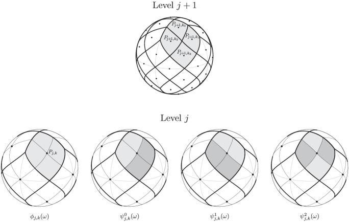
Figure 1: Haar scaling function $\phi_{j,k}(\mbox{\boldmath${\hat{s}}$})$ and wavelets $\psi_{j,k}^{m}(\mbox{\boldmath${\hat{s}}$})$. Dark shaded regions correspond to negative constant values, light shaded regions correspond to positive constant values and unshaded regions correspond to zero. The scaling function and wavelets at level $j$ and position $k$ are non-zero on pixel $P_{j,k}$ only. Pixel $P_{j,k}$ at level $j$ is subdivided into four pixels at level $j+1$, which we label $P_{j+1,k_{0}}$, $P_{j+1,k_{1}}$, $P_{j+1,k_{2}}$ and $P_{j+1,k_{3}}$ as defined above.

The non-zero value of the scaling function $1/\sqrt{A_{j}}$ is chosen to ensure that the scaling functions $\phi_{j,k}$ for $k=0,\cdots,N_{j}-1$ do indeed define an orthonormal basis for $V_{j}$. Before defining the wavelets explicitly, we fix some additional notation. Pixel $P_{j,k}$ at level $j$ is subdivided into four pixels at level $j+1$, which we label $P_{j+1,k_{0}}$, $P_{j+1,k_{1}}$, $P_{j+1,k_{2}}$ and $P_{j+1,k_{3}}$, as illustrated in Fig. 1. An orthonormal basis for the wavelet space $W_{j}$, the orthogonal complement of $V_{j}$, is then given by the following wavelets of type $m=\{0,1,2\}$:

$$\psi_{j,k}^{0}(\mbox{\boldmath${\hat{s}}$})\equiv\bigl{[}\phi_{j+1,k_{0}}(\mbox{\boldmath${\hat{s}}$})-\phi_{j+1,k_{1}}(\mbox{\boldmath${\hat{s}}$})+\phi_{j+1,k_{2}}(\mbox{\boldmath${\hat{s}}$})-\phi_{j+1,k_{3}}(\mbox{\boldmath${\hat{s}}$})\bigr{]}/2\>;$$

$$\psi_{j,k}^{1}(\mbox{\boldmath${\hat{s}}$})\equiv\bigl{[}\phi_{j+1,k_{0}}(\mbox{\boldmath${\hat{s}}$})+\phi_{j+1,k_{1}}(\mbox{\boldmath${\hat{s}}$})-\phi_{j+1,k_{2}}(\mbox{\boldmath${\hat{s}}$})-\phi_{j+1,k_{3}}(\mbox{\boldmath${\hat{s}}$})\bigr{]}/2\>;$$

$$\psi_{j,k}^{2}(\mbox{\boldmath${\hat{s}}$})\equiv\bigl{[}\phi_{j+1,k_{0}}(\mbox{\boldmath${\hat{s}}$})-\phi_{j+1,k_{1}}(\mbox{\boldmath${\hat{s}}$})-\phi_{j+1,k_{2}}(\mbox{\boldmath${\hat{s}}$})+\phi_{j+1,k_{3}}(\mbox{\boldmath${\hat{s}}$})\bigr{]}/2\>.$$

We require three independent wavelet types to construct a complete basis for $W_{j}$ since the dimension of $V_{j+1}$ (given by $N_{j+1}$) is four times larger than the dimension of $V_{j}$ (the approximation function provides the fourth component). The Haar scaling functions and wavelets defined here on the sphere are illustrated in Fig. 1.

Let us check that the scaling functions and wavelets satisfy the requirements for an orthonormal multiresolution analysis as outlined previously. We require $W_{j}$ to be orthogonal to $V_{j}$, i.e. we require

$$\int_{\mathrm{S}^{2}}\phi_{j,k}(\mbox{\boldmath${\hat{s}}$})\>\psi_{j,k^{\prime}}^{m}(\mbox{\boldmath${\hat{s}}$})\mathrm{\,d}\Omega(\mbox{\boldmath${\hat{s}}$})=0\>.$$

This is always satisfied since for $k^{\prime}\neq k$ the scaling function and wavelet do not overlap and so the integrand is zero always, and for $k^{\prime}=k$ we find

$$\int_{\mathrm{S}^{2}}\phi_{j,k}(\mbox{\boldmath${\hat{s}}$})\>\psi_{j,k}^{m}(\mbox{\boldmath${\hat{s}}$})\mathrm{\,d}\Omega(\mbox{\boldmath${\hat{s}}$})\propto\int_{\mathrm{S}^{2}}\psi_{j,k}^{m}(\mbox{\boldmath${\hat{s}}$})\mathrm{\,d}\Omega(\mbox{\boldmath${\hat{s}}$})=0\>.$$

We also require $W_{j}$ to be orthogonal to $W_{j^{\prime}}$ for all $j$ and $j^{\prime}$. Again, if the basis functions do not overlap (i.e. $k\neq k^{\prime}$) then this requirement is satisfied automatically, and if they do (i.e. $k=k^{\prime}$) then the wavelet at the finer level $j^{\prime}>j$ will always lie within a region of the wavelet at level $j$ with constant value, and consequently

$$\int_{\mathrm{S}^{2}}\psi_{j,k}^{m}(\mbox{\boldmath${\hat{s}}$})\>\psi_{{j^{\prime}},{k^{\prime}}}^{m^{\prime}}(\mbox{\boldmath${\hat{s}}$})\mathrm{\,d}\Omega(\mbox{\boldmath${\hat{s}}$})\propto\int_{\mathrm{S}^{2}}\psi_{j^{\prime},k^{\prime}}^{m^{\prime}}(\mbox{\boldmath${\hat{s}}$})\mathrm{\,d}\Omega(\mbox{\boldmath${\hat{s}}$})=0\>.$$

Finally, to ensure that we have constructed an orthonormal wavelet basis for $W_{j}$, we check the orthogonality of all wavelets at level $j$:

$$\int_{\mathrm{S}^{2}}\psi_{j,k}^{m}(\mbox{\boldmath${\hat{s}}$})\>\psi_{{j},{k^{\prime}}}^{m^{\prime}}(\mbox{\boldmath${\hat{s}}$})\mathrm{\,d}\Omega(\mbox{\boldmath${\hat{s}}$})=\delta_{{m}{m^{\prime}}}\delta_{{k}{k^{\prime}}}\>\Biggl{(}\frac{1}{2\sqrt{A_{j+1}}}\Biggr{)}^{2}\>A_{j}=\delta_{{m}{m^{\prime}}}\delta_{{k}{k^{\prime}}}\>,$$

where for $m\neq m^{\prime}$ the positive and negative regions of the integrand cancel exactly and for $k\neq k^{\prime}$ the wavelets do not overlap and so the integrand is zero always. Note that in the previous expression the final $A_{j}$ term arises from the area element. The Haar approximation and wavelet spaces that we have constructed therefore satisfy the requirements of an orthonormal multiresolution analysis on the sphere. Although the orthogonal nature of these spaces is important, a different normalisation could be chosen. It is now possible to define the analysis and synthesis of a function on the sphere in this Haar wavelet multiresolution framework.

The decomposition of a function defined on a HEALPix sphere at resolution $J$, i.e. $F_{J}\in V_{J}$, into its wavelet and scaling coefficients proceeds as follows. Consider an intermediate level $j+1<J$ and let $F_{j+1}$ be the approximation of $F_{J}$ in $V_{j+1}$. The scaling coefficients at the coarser level $j$ are given by the projection of $F_{j+1}$ onto the scaling functions $\phi_{j,k}$:

$$\lambda_{j,k} \equiv\int_{\mathrm{S}^{2}}F_{j+1}(\mbox{\boldmath${\hat{s}}$})\>\phi_{j,k}(\mbox{\boldmath${\hat{s}}$})\mathrm{\,d}\Omega(\mbox{\boldmath${\hat{s}}$})$$

$$=\bigl{(}\lambda_{j+1,k_{0}}+\lambda_{j+1,k_{1}}+\lambda_{j+1,k_{2}}+\lambda_{j+1,k_{3}}\bigr{)}\sqrt{A_{j}}/4\>,$$

where we call $\lambda_{j,k}$ the approximation coefficients since they define the approximation function $F_{j}\in V_{j}$. At the finest level $J$, we naturally associate the function values of $F_{J}$ with the approximation coefficients of this level. The wavelet coefficients at level $j$ are given by the projection of $F_{j+1}$ onto the wavelets $\psi_{j,k}^{m}$:

$$\gamma_{j,k}^{m}\equiv\int_{\mathrm{S}^{2}}F_{j+1}(\mbox{\boldmath${\hat{s}}$})\>\psi_{j,k}^{m}(\mbox{\boldmath${\hat{s}}$})\mathrm{\,d}\Omega(\mbox{\boldmath${\hat{s}}$})\>,$$

giving

$$\gamma_{j,k}^{0}=\bigl{(}\lambda_{j+1,k_{0}}-\lambda_{j+1,k_{1}}+\lambda_{j+1,k_{2}}-\lambda_{j+1,k_{3}}\bigr{)}\sqrt{A_{j}}/4\>,$$

$$\gamma_{j,k}^{1}=\bigl{(}\lambda_{j+1,k_{0}}+\lambda_{j+1,k_{1}}-\lambda_{j+1,k_{2}}-\lambda_{j+1,k_{3}}\bigr{)}\sqrt{A_{j}}/4\>$$

and

$$\gamma_{j,k}^{2}=\bigl{(}\lambda_{j+1,k_{0}}-\lambda_{j+1,k_{1}}-\lambda_{j+1,k_{2}}+\lambda_{j+1,k_{3}}\bigr{)}\sqrt{A_{j}}/4\>,$$

where we call $\gamma_{j,k}^{m}$ the detail (or wavelet) coefficients of type $m$. Starting from the finest level $J$, we compute the approximation and detail coefficients at level $J-1$ as outlined above. We then repeat this procedure to decompose the approximation coefficients at level $J-1$ (i.e. the approximation function $F_{J-1}$), into approximation and detail coefficients at the coarser level $J-2$. Repeating this procedure continually, we recover the multiresolution representation of $F_{J}$ in terms of the coarsest level approximation $F_{1}$ and all of the detail coefficients, as specified by (4) and illustrated in Fig. 2. In general it is not necessary to continue the multiresolution decomposition down to the coarsest level $j=1$; one may choose to stop at the intermediate level $J_{0}$, where $1\leq J_{0}<J$.

The function $F_{J}\in V_{J}$ may then be synthesised from its approximation and detail coefficients. Due to the orthogonal nature of the Haar basis, the approximation coefficients at level $j+1$ may be reconstructed from the weighted expansion of the scaling function and wavelets at the coarser level $j$, where the weights are given by the approximation and detail coefficients respectively. Writing this expansion explicitly, the approximation coefficients at level $j+1$ are given in terms of the approximation and detail coefficients of the coarser level $j$:

$$\lambda_{j+1,k_{0}}=\bigl{(}\lambda_{j,k}+\gamma_{j,k}^{0}+\gamma_{j,k}^{1}+\gamma_{j,k}^{2}\bigr{)}/\sqrt{A_{j}}\>;$$

$$\lambda_{j+1,k_{1}}=\bigl{(}\lambda_{j,k}-\gamma_{j,k}^{0}+\gamma_{j,k}^{1}-\gamma_{j,k}^{2}\bigr{)}/\sqrt{A_{j}}\>;$$

$$\lambda_{j+1,k_{2}}=\bigl{(}\lambda_{j,k}+\gamma_{j,k}^{0}-\gamma_{j,k}^{1}-\gamma_{j,k}^{2}\bigr{)}/\sqrt{A_{j}}\>;$$

$$\lambda_{j+1,k_{3}}=\bigl{(}\lambda_{j,k}-\gamma_{j,k}^{0}-\gamma_{j,k}^{1}+\gamma_{j,k}^{2}\bigr{)}/\sqrt{A_{j}}\>.$$

Repeating this procedure from level $j=J_{0}$ up to $j=J$, one finds that the signal $F_{J}\in V_{J}$ may be written as the scaling function and wavelet expansion

$$F_{J}(\mbox{\boldmath${\hat{s}}$})=\sum_{k=0}^{N_{J_{0}}-1}\lambda_{J_{0},k}\>\phi_{J_{0},k}(\mbox{\boldmath${\hat{s}}$})+\sum_{j=J_{0}}^{J-1}\sum_{k=0}^{N_{j}-1}\sum_{m=0}^{2}\gamma_{j,k}^{m}\>\psi_{j,k}^{m}(\mbox{\boldmath${\hat{s}}$})\>.$$ (5)

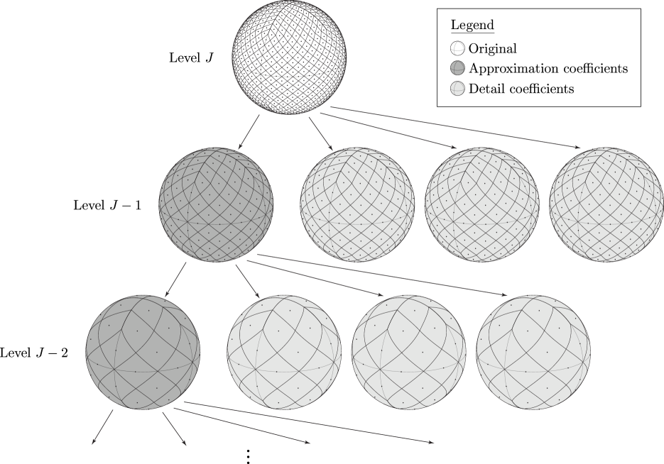
Figure 2: Haar multiresolution decomposition. Starting at the finest level $J$ (the original sphere), the approximation and detail coefficients at level $J-1$ are computed. This procedure is repeated to decompose the approximation coefficients at level $J-1$ (i.e. the approximation function $F_{J-1}$), into approximation and detail coefficients at the coarser level $J-2$. Repeating this procedure continually, one recovers the multiresolution representation of $F_{J}$ in terms of the coarsest level approximation $F_{J_{0}}$ and all of the detail coefficients.

2.3 Rotations

Rotations $\mathcal{R}$ on the sphere are characterised by the elements of the rotation group ${\mathrm{SO}(3)}$, which we parameterise in terms of the three Euler angles $\rho=(\alpha,\beta,\gamma)\in{\mathrm{SO}(3)}$, where $\alpha\in[0,2\pi)$, $\beta\in[0,\pi]$ and $\gamma\in[0,2\pi)$. The rotation of a coordinate vector ${\hat{s}}$ by $\mathcal{R}(\mathbf{\rho})$ may be represented by multiplication of the Cartesian coordinate with the 3$\times$3 rotation matrix $\mathbf{R}(\mathbf{\rho})$. We adopt the $zyz$ Euler convention corresponding to the rotation of a physical body in a fixed coordinate system about the $z$, $y$ and $z$ axes by $\gamma$, $\beta$ and $\alpha$ respectively, i.e. $\mathbf{R}(\mathbf{\rho})=\mathbf{R}_{z}(\alpha)\mathbf{R}_{y}(\beta)\mathbf{R}_{z}(\gamma)$, where $\mathbf{R}_{z}(\vartheta)$ and $\mathbf{R}_{y}(\vartheta)$ are rotation matrices representing rotations by $\vartheta$ about the $z$ and $y$ axis respectively. The inverse rotation is given by $\mathbf{R}^{-1}(\mathbf{\rho})=\mathbf{R}_{z}(-\gamma)\mathbf{R}_{y}(-\beta)\mathbf{R}_{z}(-\alpha)$. We define the rotation of a function $F\in\mathrm{L}^{2}({\mathrm{S}^{2}},\mathrm{\,d}\Omega)$ on the sphere by

$$\bigl{(}\mathcal{R}(\mathbf{\rho})F\bigr{)}(\mbox{\boldmath${\hat{s}}$})=F\bigl{(}\mathbf{R}^{-1}(\mathbf{\rho})\mbox{\boldmath${\hat{s}}$}\bigr{)}\>.$$ (6)

It is also useful to characterise the rotation of a function on the sphere in harmonic space. The Wigner $D$-functions $D_{mn}^{\ell}(\mathbf{\rho})$ provide the irreducible unitary representation of the rotation group ${\mathrm{SO}(3)}$. For our purpose, we merely consider the Wigner $D$-functions to represent the rotation of a function on the sphere in harmonic space. The rotation of a spherical harmonic basis function may be represented by a sum of weighted harmonics of the same $\ell$ (Brink & Satchler, 1999): $\bigl{(}\mathcal{R}(\mathbf{\rho})Y_{\ell m}\bigr{)}(\mbox{\boldmath${\hat{s}}$})=\sum_{n=-\ell}^{\ell}D_{nm}^{\ell}(\mathbf{\rho})\>Y_{\ell n}({\mbox{\boldmath${\hat{s}}$}})$. It is then trivial to show that the harmonic coefficients of a rotated function are related to the coefficients of the original function by

$$\bigl{(}\mathcal{R}(\mathbf{\rho})F\bigr{)}_{\ell m}=\sum_{n=-\ell}^{\ell}D_{mn}^{\ell}(\mathbf{\rho})\>F_{\ell n}\>.$$ (7)

For computational purposes, the Wigner functions may be decomposed as $D_{mn}^{\ell}(\alpha,\beta,\gamma)={\rm e}^{-{\rm i}m\alpha}\>d_{mn}^{\ell}(\beta)\>{\rm e}^{-{\rm i}n\gamma}$, where the real polar $d$-functions are defined by Varshalovich et al. (1989). Recursion formulae exist to compute the Wigner $d$-functions rapidly (Risbo, 1996).

3 Full-sky interferometry

We formulate full-sky interferometry in this section in real, spherical harmonic and SHW spaces. Since we treat interferometry in the full-sky setting it is necessary to be explicit about the coordinate systems used and the relations between them. After discussing the various coordinate systems that we use, we describe visibility computation and image reconstruction for the representation of interferometry in each space, highlighting the relative merits of each representation. These ideas are then extended to incorporate horizon occlusion and primary beam functions that depend on the interferometer pointing direction.

3.1 Coordinate systems

The complex visibility measured by an interferometer is given by the coordinate free definition (Thompson et al., 2001)

$$\mathcal{V}(\mbox{\boldmath${u}$})=\int_{\mathrm{S}^{2}}A(\mbox{\boldmath${\sigma}$})I(\mbox{\boldmath${\sigma}$}){\rm e}^{-{\rm i}2\pi\mbox{\boldmath${u}$}\cdot\mbox{\boldmath${\sigma}$}}\mathrm{\,d}\Omega\>,$$ (8)

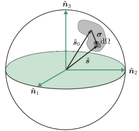
Figure 3: Geometry of an observation of an extended source centred at the interferometer pointing direction $\mbox{\boldmath${\hat{s}}$}_{0}$. The area element $\mathrm{\,d}\Omega$ represents the contribution to the visibility integral from point ${\hat{s}}$. The full visibility is obtained by summing all such contributions over the sky. Note that the sky has been mapped onto the unit celestial sphere, hence ${\hat{s}}$ and $\mbox{\boldmath${\hat{s}}$}_{0}$ are unit vectors.

where $\mbox{\boldmath${\sigma}$}=\mbox{\boldmath${\hat{s}}$}-\mbox{\boldmath${\hat{s}}$}_{0}$; the area element $\mathrm{\,d}\Omega$ and the vectors ${\sigma}$, ${\hat{s}}$ and $\mbox{\boldmath${\hat{s}}$}_{0}$ are defined in Fig. 3. We assume that the sky is mapped onto the unit celestial sphere, hence all vectors on the sphere are unit vectors. The vector ${u}$ is related to the baseline of the interferometer (and is defined explicitly later), the function $A$ defines the primary beam of the interferometer and the function $I$ defines the intensity of the sky at position ${\sigma}$. In this coordinate free definition of visibility, ${\sigma}$ is essentially the representation of ${\hat{s}}$ in a coordinate system centred on $\mbox{\boldmath${\hat{s}}$}_{0}$. The translation $\mbox{\boldmath${\sigma}$}=\mbox{\boldmath${\hat{s}}$}-\mbox{\boldmath${\hat{s}}$}_{0}$ represents the transformation between the global coordinate frame of ${\hat{s}}$ and the local coordinate frame of ${\sigma}$. In general, one can transform vectors between global coordinates and local coordinates relative to $\mbox{\boldmath${\hat{s}}$}_{0}$, through a rotation by $\mbox{\boldmath${\hat{s}}$}_{0}$. We now formalise this notion.

Let us define two coordinate frames. The global coordinate frame of the celestial sky is defined by the right handed set of unit vectors $\{\hat{\mbox{\boldmath${n}$}}_{1},\hat{\mbox{\boldmath${n}$}}_{2},\hat{\mbox{\boldmath${n}$}}_{3}\}$. The local coordinate frame relative to $\mbox{\boldmath${\hat{s}}$}_{0}$ is defined by the right handed set of unit vectors $\{\hat{\mbox{\boldmath${u}$}}_{1},\hat{\mbox{\boldmath${u}$}}_{2},\hat{\mbox{\boldmath${u}$}}_{3}\}$, where $\hat{\mbox{\boldmath${u}$}}_{3}$ aligns with $\mbox{\boldmath${\hat{s}}$}_{0}$. These two coordinate frames are related by the rotation $\mathcal{R}_{0}\equiv\mathcal{R}(\varphi_{0},\theta_{0},0)$, where $(\theta_{0},\varphi_{0})$ are the spherical coordinates of $\mbox{\boldmath${\hat{s}}$}_{0}$ in the global coordinate frame. The corresponding $3\times 3$ rotation matrix $\mathbf{R}_{0}\equiv\mathbf{R}(\varphi_{0},\theta_{0},0)$ transforms a vector between local and global coordinates. For example, $\mbox{\boldmath${\hat{s}}$}_{0}$ in global coordinates corresponds to $\hat{\mbox{\boldmath${u}$}}_{3}$ in local coordinates (by definition) and the two vectors are related by $\mbox{\boldmath${\hat{s}}$}_{0}=\mathbf{R}_{0}\hat{\mbox{\boldmath${u}$}}_{3}$. In general, local coordinates are related to global coordinates by $\mbox{\boldmath${\hat{s}}$}^{{\rm l}}=\mathbf{R}_{0}^{-1}\mbox{\boldmath${\hat{s}}$}^{{\rm n}}$, where the superscripts ${\rm l}$ and ${\rm n}$ denote local and global coordinates respectively; henceforth all vectors and functions contain an ${\rm l}$ or ${\rm n}$ superscript to denote their coordinate frame. The third Euler angle of the rotation mapping local to global coordinates specifies an azimuthal rotation around $\mbox{\boldmath${\hat{s}}$}_{0}$, which is in general arbitrary but fixed. Without loss of generality we set this third Euler angle to zero. Fig. 4 illustrates the rotation that transforms between local and global coordinates.

Returning to the visibility function, we may now represent this in the coordinate frames defined above. The beam function is most naturally represented in local coordinates relative to the pointing direction $\mbox{\boldmath${\hat{s}}$}_{0}^{{\rm n}}$. We denote this function by $A^{\rm l}(\mbox{\boldmath${\hat{s}}$}^{{\rm l}})\in\mathrm{L}^{2}({\mathrm{S}^{2}},\mathrm{\,d}\Omega)$. The source intensity function is most naturally represented in global coordinates and is denoted by $I^{\rm n}(\mbox{\boldmath${\hat{s}}$}^{{\rm n}})\in\mathrm{L}^{2}({\mathrm{S}^{2}},\mathrm{\,d}\Omega)$. We may convert a function $F^{\rm n}$ in global coordinates to a corresponding function $F^{\rm l}$ in local coordinates through the rotation $\mathcal{R}_{0}$:

$$F^{\rm n}(\mbox{\boldmath${\hat{s}}$}^{{\rm n}})=F^{\rm n}(\mathbf{R}_{0}\mbox{\boldmath${\hat{s}}$}^{{\rm l}})=(\mathcal{R}_{0}^{-1}F^{\rm n})(\mbox{\boldmath${\hat{s}}$}^{{\rm l}})=F^{\rm l}(\mbox{\boldmath${\hat{s}}$}^{{\rm l}})\>,$$

i.e. $F^{\rm l}=\mathcal{R}_{0}^{-1}F^{\rm n}$. In practice, sampled functions on the sphere may be rotated in real space through (6) or alternatively, and more accurately (since pixelisation artifacts are eliminated), in harmonic space through (7). In this coordinate setting the visibility integral may be written

$$\mathcal{V}(\mbox{\boldmath${u}$})=\int_{\mathrm{S}^{2}}A^{\rm l}(\mbox{\boldmath${\hat{s}}$}^{{\rm l}})\>I^{\rm n}(\mbox{\boldmath${\hat{s}}$}^{{\rm n}})\>{\rm e}^{-{\rm i}2\pi\mbox{\boldmath${u}$}\cdot\mbox{\boldmath${\hat{s}}$}^{{\rm l}}}\mathrm{\,d}\Omega(\mbox{\boldmath${\hat{s}}$}^{{\rm l}})\>.$$

When dealing with the visibility integral it is more convenient to represent all functions in the same coordinate frame. In local coordinates the visibility integral becomes

$$\mathcal{V}(\mbox{\boldmath${u}$}) =\int_{\mathrm{S}^{2}}A^{\rm l}(\mbox{\boldmath${\hat{s}}$}^{{\rm l}})\>(\mathcal{R}_{0}^{-1}I^{\rm n})(\mbox{\boldmath${\hat{s}}$}^{{\rm l}})\>{\rm e}^{-{\rm i}2\pi\mbox{\boldmath${u}$}\cdot\mbox{\boldmath${\hat{s}}$}^{{\rm l}}}\mathrm{\,d}\Omega(\mbox{\boldmath${\hat{s}}$}^{{\rm l}})$$

$$=\int_{\mathrm{S}^{2}}A^{\rm l}(\mbox{\boldmath${\hat{s}}$}^{{\rm l}})\>I^{\rm l}(\mbox{\boldmath${\hat{s}}$}^{{\rm l}})\>{\rm e}^{-{\rm i}2\pi\mbox{\boldmath${u}$}\cdot\mbox{\boldmath${\hat{s}}$}^{{\rm l}}}\mathrm{\,d}\Omega(\mbox{\boldmath${\hat{s}}$}^{{\rm l}})\>.$$ (9)

Here ${u}$ is the interferometer baseline in local coordinates (an explicit expression for ${u}$ is deferred until the more general formulation presented in Sec. 3.4). The expression given by (3.1) is the familiar interferometric visibility integral, however in discussing this integral in the full-sky setting it has been necessary to make the use of different coordinate systems explicit. To compute visibilities when including contributions over the entire sky, one could simply evaluate (3.1) by using an appropriate quadrature rule on the sphere. The complexity of evaluating this integral directly for a single baseline ${u}$ scales as $\mathcal{O}(N)$ (recall that $N$ is the number of pixels contained in the pixelisation of the sphere). Low-resolution simulations of full-sky interferometric observations are computed in this manner in Sec. 4.

We also define the coordinate system $\mbox{\boldmath${p}$}=(p,q)$ on the tangent plane of the celestial sphere at the pointing direction. This coordinate system is used to define the image plane when reconstructing images on small patches using the standard Fourier transform approach and is obviously a local coordinate frame. It is related to the spherical coordinates $(\theta^{\rm l},\varphi^{\rm l})$ of the local $\{\hat{\mbox{\boldmath${u}$}}_{1},\hat{\mbox{\boldmath${u}$}}_{2},\hat{\mbox{\boldmath${u}$}}_{3}\}$ frame by $p=\sin\theta^{\rm l}\cos\varphi^{\rm l}$ and $q=\sin\theta^{\rm l}\sin\varphi^{\rm l}$.

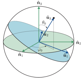
Figure 4: Rotation $\mathcal{R}_{0}$ mapping global coordinates of the celestial sky defined in the frame $\{\hat{\mbox{\boldmath${n}$}}_{1},\hat{\mbox{\boldmath${n}$}}_{2},\hat{\mbox{\boldmath${n}$}}_{3}\}$ to local coordinates defined in the frame $\{\hat{\mbox{\boldmath${u}$}}_{1},\hat{\mbox{\boldmath${u}$}}_{2},\hat{\mbox{\boldmath${u}$}}_{3}\}$, where $\hat{\mbox{\boldmath${u}$}}_{3}$ is aligned with $\mbox{\boldmath${\hat{s}}$}_{0}$. Local coordinates are related to global coordinates by $\mbox{\boldmath${\hat{s}}$}^{{\rm l}}=\mathbf{R}_{0}^{-1}\mbox{\boldmath${\hat{s}}$}^{{\rm n}}$.

3.2 Spherical harmonic space representation

It is more general and accurate to compute the visibility integral in harmonic space since this avoids the need for any quadrature rule on the sphere, which would necessarily be pixelisation dependent and not always exact. Moreover, rotations can be performed through (7) in harmonic space more accurately than they can be performed in real space. We derive here the spherical harmonic representation of the visibility integral and discuss the implications of this representation for computing visibilities and for image reconstruction.

3.2.1 Computing visibilities

Consider the beam-modulated source intensity function $\mbox{$\bigl{(}A^{\rm l}\cdot I^{\rm l}\bigr{)}$}(\mbox{\boldmath${\hat{s}}$}^{{\rm l}})=A^{\rm l}(\mbox{\boldmath${\hat{s}}$}^{{\rm l}})I^{\rm l}(\mbox{\boldmath${\hat{s}}$}^{{\rm l}})$. Substituting the spherical harmonic expansion of this function into the local coordinate visibility integral given by (3.1), we obtain

$$\mathcal{V}(\mbox{\boldmath${u}$})=\sum_{\ell m}{\mbox{$\bigl{(}A^{\rm l}\cdot I^{\rm l}\bigr{)}$}}_{{\ell}{m}}\int_{\mathrm{S}^{2}}{\rm e}^{-{\rm i}2\pi\mbox{\boldmath${u}$}\cdot\mbox{\boldmath${\hat{s}}$}^{{\rm l}}}\>Y_{\ell m}({\mbox{\boldmath${\hat{s}}$}^{{\rm l}}})\mathrm{\,d}\Omega(\mbox{\boldmath${\hat{s}}$}^{{\rm l}})\>,$$ (10)

where ${\mbox{$\bigl{(}A^{\rm l}\cdot I^{\rm l}\bigr{)}$}}_{{\ell}{m}}$ are the spherical harmonic coefficients of the beam-modulated intensity function. We assume that the beam-modulated intensity function is band-limited at ${\ell_{\rm max}}$ so that all higher frequency harmonic coefficients are zero, i.e. ${\mbox{$\bigl{(}A^{\rm l}\cdot I^{\rm l}\bigr{)}$}}_{{\ell}{m}}=0$, $\forall\ell>{\ell_{\rm max}}$. In this case sums over the harmonic index $\ell$ may be truncated at ${\ell_{\rm max}}$. Here, and subsequently, we use the shorthand notation $\sum_{\ell m}\equiv\sum_{\ell=0}^{{\ell_{\rm max}}}\sum_{m=-\ell}^{\ell}$. The integral contained in (10) may be evaluated analytically. Noting the addition theorem for spherical harmonics and the Jacobi-Anger expansion of a plane wave given by (1) and (2) respectively, we find

$${\rm e}^{{\rm i}2\pi\mbox{\boldmath${u}$}\cdot\mbox{\boldmath${\hat{s}}$}^{{\rm l}}}=4\pi\sum_{\ell m}{\rm i}^{\ell}\>j_{\ell}(2\pi\|\mbox{\boldmath${u}$}\|)\>Y_{\ell m}^{\ast}({\hat{\mbox{\boldmath${u}$}}})\>Y_{\ell m}({\mbox{\boldmath${\hat{s}}$}^{{\rm l}}})\>.$$ (11)

Using this result, the integral contained in (10) becomes

$$\int_{\mathrm{S}^{2}}{\rm e}^{-{\rm i}2\pi\mbox{\boldmath${u}$}\cdot\mbox{\boldmath${\hat{s}}$}^{{\rm l}}}\>Y_{\ell m}({\mbox{\boldmath${\hat{s}}$}^{{\rm l}}})\mathrm{\,d}\Omega(\mbox{\boldmath${\hat{s}}$}^{{\rm l}})=4\pi\>(-{\rm i})^{\ell}\>j_{\ell}(2\pi\|\mbox{\boldmath${u}$}\|)\>Y_{\ell m}({\mbox{\boldmath${\hat{\mbox{\boldmath${u}$}}}$}})\>,$$

where we have noted the orthogonality of the spherical harmonics. The harmonic representation of the visibility function then reads

$$\mathcal{V}(\mbox{\boldmath${u}$})=4\pi\sum_{\ell m}(-{\rm i})^{\ell}\>j_{\ell}(2\pi\|\mbox{\boldmath${u}$}\|)\>Y_{\ell m}({\mbox{\boldmath${\hat{\mbox{\boldmath${u}$}}}$}})\>{\mbox{$\bigl{(}A^{\rm l}\cdot I^{\rm l}\bigr{)}$}}_{{\ell}{m}}\>.$$ (12)

This expression has been derived independently by Ng (2001) to study properties of the angular power spectrum recovered from interferometric observations of the CMB, however slightly different definition are adopted to those used here.

Computing visibilities using (12) ensures that full-sky contributions from the beam-modulated intensity function to the visibility integral are incorporated, thus allowing for arbitrarily wide fields of view and beam sizes. The complexity of evaluating (12) for a single baseline ${u}$ scales as $\mathcal{O}({\ell_{\rm max}}^{2})$, where $\mathcal{O}({\ell_{\rm max}}^{2})\sim\mathcal{O}(N)$ (as discussed in more detail in Sec. 4.1). Low-resolution simulations of full-sky interferometric observations are computed in this manner in Sec. 4.

3.2.2 Image reconstruction

In theory one may recover a full-sky synthesised image from the spherical harmonic representation of the visibility function by integration over a spherical surface in $\mathbb{R}^{3}$. We describe this approach before discussing its limitations.

It is possible to recover the beam-modulated intensity function by taking the spherical harmonic transform of the visibility function over a spherical surface at radius $\|\mbox{\boldmath${u}$}\|$. By substituting the harmonic representation of the visibility function given by (12) into the spherical harmonic transform of the visibility one finds

$$\int_{\mathrm{S}^{2}}\mathcal{V}(\mbox{\boldmath${u}$})\>Y_{\ell m}^{\ast}({\hat{\mbox{\boldmath${u}$}}})\>\mathrm{\,d}\Omega(\hat{\mbox{\boldmath${u}$}})=4\pi\>(-{\rm i})^{\ell}\>j_{\ell}(2\pi\|\mbox{\boldmath${u}$}\|)\>{\mbox{$\bigl{(}A^{\rm l}\cdot I^{\rm l}\bigr{)}$}}_{{\ell}{m}},$$ (13)

where we have noted the orthogonality of the spherical harmonics. In theory, (13) can be used to recover the harmonic coefficients of the beam-modulated intensity, from which the real space function can be reconstructed easily. In this framework, one recovers the beam-modulated intensity on the entire sky, arbitrarily far from the interferometer pointing direction. However, there are a number of limitations of this approach that render it infeasible in practice.

To recover the harmonic coefficients ${\mbox{$\bigl{(}A^{\rm l}\cdot I^{\rm l}\bigr{)}$}}_{{\ell}{m}}$ from (13) we require that $j_{\ell}(2\pi\|\mbox{\boldmath${u}$}\|)$ is non-zero for the particular value of $\ell$ and the radius $\|\mbox{\boldmath${u}$}\|$ considered. Firstly, let us attempt to recover ${\mbox{$\bigl{(}A^{\rm l}\cdot I^{\rm l}\bigr{)}$}}_{{\ell}{m}}$ for all $\ell$ and $m$ from a spherical sampling of the visibility function at a single radius $\|\mbox{\boldmath${u}$}\|$. In theory this is possible since the $z$th zeros of the spherical Bessel function are strictly monotonically increasing with order $\ell$ (Liu & Zou, 2007), hence by choosing a value of $2\pi\|\mbox{\boldmath${u}$}\|$ that lies between two zeros of identical zero-order $z$ and adjacent function-order $\ell$, we ensure that we avoid all zeros of the spherical Bessel functions. Nevertheless, as the order $\ell$ deviates from the adjacent values chosen, the spherical Bessel functions will become arbitrarily closer to zero. Consequently, any numerical attempts to recover ${\mbox{$\bigl{(}A^{\rm l}\cdot I^{\rm l}\bigr{)}$}}_{{\ell}{m}}$ using this procedure will be unstable. A full ${u}$ sampling of the visibility function in $\mathbb{R}^{3}$ is therefore required to recover the full-sky beam-modulated intensity function. For each value of $\ell$, sampled spherical surfaces with different radii should be used. The value $2\pi\|\mbox{\boldmath${u}$}\|$ used for a particular $\ell$ should be chosen to ensure that it does not lie on or near the zeros of the spherical Bessel function $j_{\ell}(2\pi\|\mbox{\boldmath${u}$}\|)$, and ideally at a low-order local extremum of the spherical Bessel function.

We have demonstrated that it is possible to recover the beam-modulated intensity over the entire sky in theory, however to do this we require full sampling of the visibility function in $\mathbb{R}^{3}$. For interferometric observations, as the field of view rotates over the sky with time we sample the visibility function for various values of the baseline in local coordinates. Typically these samples lie on a series of $uv$-tracks in the $\mbox{\boldmath${u}$}=(u,v,w)$ space for values of $w$ close to zero. For low pointing directions we recover samples at values of $w$ further from zero, but we are unlikely in practice to recover sufficient sampling of the visibility function to reconstruct the beam-modulated intensity function over the entire sky. Consequently, we do not advocate the use of the spherical harmonic representations derived above for image recovery.

3.3 Spherical Haar wavelet space representation

The main challenges that arise from the full-sky interferometry formulations in both real and spherical harmonic space are related to the localisation of signal characteristics. In real space we achieve good spatial localisation but poor frequency localisation; in spherical harmonic space we achieve good frequency localisation but poor spatial localisation. Both the primary beam and the sky intensity functions are characterised by spatially localised high frequency content, thus neither real nor harmonic space bases provide an efficient representation of these functions. However, these functions can be represented efficiently in a wavelet basis due to the simultaneous spatial and scale localisation afforded by a wavelet analysis (as discussed in Sec. 2.2). We derive here the SHW representation of the interferometry integral and discuss the implications of this representation for computing visibilities and for image reconstruction.

3.3.1 Computing visibilities

Consider the SHW representation of the beam-modulated intensity function

$$\mbox{$\bigl{(}A^{\rm l}\cdot I^{\rm l}\bigr{)}$}(\mbox{\boldmath${\hat{s}}$}^{{\rm l}})=\sum_{k=0}^{N_{J_{0}}-1}\lambda_{J_{0},k}\>\phi_{J_{0},k}(\mbox{\boldmath${\hat{s}}$}^{{\rm l}})+\sum_{j=J_{0}}^{J-1}\sum_{k=0}^{N_{j}-1}\sum_{m=0}^{2}\gamma_{j,k}^{m}\>\psi_{j,k}^{m}(\mbox{\boldmath${\hat{s}}$}^{{\rm l}})\>,$$ (14)

where $\lambda_{J_{0},k}$ and $\gamma_{j,k}^{m}$ are the scaling and wavelet coefficients of the beam-modulated intensity function respectively, and the SHW representation of the plane wave

$${\rm e}^{-{\rm i}2\pi\mbox{\boldmath${u}$}\cdot\mbox{\boldmath${\hat{s}}$}^{{\rm l}}}=\sum_{k=0}^{N_{J_{0}}-1}\eta_{J_{0},k}(\mbox{\boldmath${u}$})\>\phi_{J_{0},k}(\mbox{\boldmath${\hat{s}}$}^{{\rm l}})+\sum_{j=J_{0}}^{J-1}\sum_{k=0}^{N_{j}-1}\sum_{m=0}^{2}\delta_{j,k}^{m}(\mbox{\boldmath${u}$})\>\psi_{j,k}^{m}(\mbox{\boldmath${\hat{s}}$}^{{\rm l}})\>,$$ (15)

where $\eta_{J_{0},k}$ and $\delta_{j,k}^{m}$ are the scaling and wavelet coefficients of the plane wave respectively. Substituting these expansions into the local coordinate visibility integral given by (3.1), we obtain

$$\mathcal{V}(\mbox{\boldmath${u}$})=\sum_{k=0}^{N_{J_{0}}-1}\sum_{k^{\prime}=0}^{N_{J_{0}}-1}\lambda_{J_{0},k}\>\eta_{J_{0},k^{\prime}}(\mbox{\boldmath${u}$})\int_{\mathrm{S}^{2}}\phi_{J_{0},k}(\mbox{\boldmath${\hat{s}}$}^{{\rm l}})\>\phi_{J_{0},k^{\prime}}(\mbox{\boldmath${\hat{s}}$}^{{\rm l}})\mathrm{\,d}\Omega(\mbox{\boldmath${\hat{s}}$}^{{\rm l}})$$

$$\,+\sum_{k=0}^{N_{J_{0}}-1}\sum_{j^{\prime}=J_{0}}^{J-1}\sum_{k^{\prime}=0}^{N_{j^{\prime}}-1}\sum_{m^{\prime}=0}^{2}\lambda_{J_{0},k}\>\delta_{j^{\prime},k^{\prime}}^{m^{\prime}}(\mbox{\boldmath${u}$})\int_{\mathrm{S}^{2}}\phi_{J_{0},k}(\mbox{\boldmath${\hat{s}}$}^{{\rm l}})\>\psi_{j^{\prime},k^{\prime}}^{m^{\prime}}(\mbox{\boldmath${\hat{s}}$}^{{\rm l}})\mathrm{\,d}\Omega(\mbox{\boldmath${\hat{s}}$}^{{\rm l}})$$

$$\,+\sum_{j=J_{0}}^{J-1}\sum_{k=0}^{N_{j}-1}\sum_{m=0}^{2}\sum_{k^{\prime}=0}^{N_{J_{0}}-1}\gamma_{j,k}^{m}\>\eta_{J_{0},k^{\prime}}(\mbox{\boldmath${u}$})\int_{\mathrm{S}^{2}}\psi_{j,k}^{m}(\mbox{\boldmath${\hat{s}}$}^{{\rm l}})\>\phi_{J_{0},k^{\prime}}(\mbox{\boldmath${\hat{s}}$}^{{\rm l}})\mathrm{\,d}\Omega(\mbox{\boldmath${\hat{s}}$}^{{\rm l}})$$

$$\,+\sum_{j=J_{0}}^{J-1}\sum_{k=0}^{N_{j}-1}\sum_{m=0}^{2}\sum_{j^{\prime}=J_{0}}^{J-1}\sum_{k^{\prime}=0}^{N_{j^{\prime}}-1}\sum_{m^{\prime}=0}^{2}\gamma_{j,k}^{m}\>\delta_{j^{\prime},k^{\prime}}^{m^{\prime}}(\mbox{\boldmath${u}$})\int_{\mathrm{S}^{2}}\psi_{j,k}^{m}(\mbox{\boldmath${\hat{s}}$}^{{\rm l}})\>\psi_{j^{\prime},k^{\prime}}^{m^{\prime}}(\mbox{\boldmath${\hat{s}}$}^{{\rm l}})\mathrm{\,d}\Omega(\mbox{\boldmath${\hat{s}}$}^{{\rm l}}).$$

Noting the orthogonality of the scaling functions and wavelets this reduces to

$$\mathcal{V}(\mbox{\boldmath${u}$})=\sum_{k=0}^{N_{J_{0}}-1}\lambda_{J_{0},k}\>\eta_{J_{0},k}(\mbox{\boldmath${u}$})+\sum_{j=J_{0}}^{J-1}\sum_{k=0}^{N_{j}-1}\sum_{m=0}^{2}\gamma_{j,k}^{m}\>\delta_{j,k}^{m}(\mbox{\boldmath${u}$})\>.$$ (16)

Applying (16) naively to compute visibilities in the full-sky setting is no more efficient than computing visibilities in real or harmonic space and scales as $\mathcal{O}(N)$ (since the multiresolution SHW decomposition contains exactly as many scaling and wavelet coefficients as the number of pixels on the original sphere). Furthermore, to compute (16) one must first compute the wavelet coefficients of the plane wave though (15), for each baseline ${u}$. The spherical harmonics define a natural harmonic representation on the sphere, arising from the solution to Laplace’s equation in spherical coordinates. Consequently, the expansion of the plane wave ${\rm e}^{{\rm i}2\pi\mbox{\boldmath${u}$}\cdot\mbox{\boldmath${\hat{s}}$}}$ can be performed analytically in the spherical harmonic basis through (11). Unfortunately this is not possible in the SHW basis and the scaling and wavelet coefficients of the plane wave must be computed numerically, introducing an additional overhead when computing visibilities in SHW space. However, these disadvantages are more than offset by the efficient representation of the beam-modulated intensity function in SHW space. Beam-modulated intensity functions are likely to contain localised high-frequency content and hence will be extremely sparse in the wavelet basis, i.e. a large number of wavelet coefficients will be zero. If we consider only the non-zero wavelet coefficients when computing (16), visibilities can be computed at substantially lower computational expense. Due to the pairing of approximation and detail coefficients in (16), it is also only necessary to compute the scaling and wavelet coefficients of the plane wave that correspond to the non-zero coefficients of the beam-modulated intensity function, thus reducing the overhead discussed above. Although it is not possible to determine exactly how (16) scales with the resolution of the pixelised spheres considered, since this depends on the SHW sparsity properties of the particular beam-modulated intensity function considered, the complexity of computing (16) is found (see Sec. 4) to something scale like $\mathcal{O}({\ell_{\rm max}}^{n})$, where $n\lesssim 1$.

In practice, not only are many of the SHW coefficients of the beam-modulated intensity identically zero, but many are also very close to zero. These wavelet coefficients contain minimal information content and can be set identically to zero without introducing substantial errors in the representation of the original beam-modulated intensity function on the sphere. For practical implementations a strategy is required to determine those wavelet coefficients that are sufficiently close to zero that they can be safely ignored. We develop two such strategies. The first strategy involves simple hard thresholding, so that all wavelet coefficients below a threshold (in absolute value) are ignored. The threshold value is determined by specifying the proportion of wavelet coefficients to retain. Typically less than one percent of the wavelet coefficients can be kept while still ensuring visibilities are computed accurately, as we shall see in Sec. 4. This strategy treats all of the wavelet coefficients identically. However, wavelet coefficients on coarser levels (lower $j$) are defined over a larger portion of the sky and so contain more information content. One should therefore favour keeping wavelet coefficients at coarser levels over finer levels. Our second strategy for determining the wavelet coefficients to retain is based on hard thresholding with an annealing strategy to determine the threshold value separately for each level $j$. The proportion of coefficients to retain at the finest level is specified and this proportion is increased quadratically as ones progresses to coarser levels. We also experimented with linear and exponential annealing strategies, however the quadratic strategy was most successful in characterising the importance of wavelet coefficients across levels.

In Sec. 4 low-resolution simulations of full-sky interferometric observations are computed using the SHW method outlined here. Due to the superior computational efficiency of the SHW method compared to the real and spherical harmonic space approaches, it is also possible to perform high-resolution simulations of interferometric observations using this method; these are also presented in Sec. 4.

3.3.2 Image reconstruction

In the SHW formulation of full-sky interferometry given by (16), the scaling and wavelet coefficients of the beam-modulated intensity function are linearly related to the visibilities by the scaling and wavelet coefficients of the plane wave. The plane wave is oscillatory and does not contain localised high frequency content, hence the plane wave is not likely to be sparsely represented in the SHW basis. Consequently, the use of (16) for wide field of view image reconstruction is much more well posed than the spherical harmonic representation of the visibility integral. Furthermore, if the primary beam is known, which is often the case, then one need only attempt to recover the wavelet coefficients of the beam-modulated intensity function that correspond to the non-zero coefficients of the primary beam, i.e. the beam tells us exactly which wavelet coefficients to recover and all others can safely be assumed to be zero.

SHW image reconstruction on the full-sky therefore involves inverting the linear system given by (16). To solve this system is it instructive to write it as the matrix equation

$$\mathcal{V}(\mbox{\boldmath${u}$})=\begin{bmatrix}\mn@boldsymbol{\eta}_{J_{0}}(\mbox{\boldmath${u}$})\\ \mn@boldsymbol{\delta}(\mbox{\boldmath${u}$})\end{bmatrix}^{\rm T}\begin{bmatrix}\mn@boldsymbol{\lambda}_{J_{0}}\\ \mn@boldsymbol{\gamma}\end{bmatrix}=\Delta^{\rm T}(\mbox{\boldmath${u}$})\>\mn@boldsymbol{\Gamma}\>,$$

where $\mn@boldsymbol{\lambda}_{J_{0}}$ and $\mn@boldsymbol{\gamma}$ are vectors of concatenated non-zero scaling and wavelet coefficients of the beam-modulated intensity and $\mn@boldsymbol{\eta}_{J_{0}}(\mbox{\boldmath${u}$})$ and $\mn@boldsymbol{\delta}(\mbox{\boldmath${u}$})$ are the corresponding coefficients of the plane wave. Combining the scaling and detail coefficients into a single vector we obtain $\mn@boldsymbol{\Gamma}=[\mn@boldsymbol{\lambda}_{J_{0}}\,\,\mn@boldsymbol{\gamma}]^{\rm T}$ and $\mn@boldsymbol{\Delta}(\mbox{\boldmath${u}$})=[\mn@boldsymbol{\eta}_{J_{0}}(\mbox{\boldmath${u}$})\,\,\mn@boldsymbol{\delta}(\mbox{\boldmath${u}$})]^{\rm T}$. Now assuming that we have $M$ visibility observations corresponding to different baselines, we may write the system of equations that we recover as the single matrix equation

$$\mn@boldsymbol{\mathcal{V}}=\mathbf{M}^{\rm T}\>\mn@boldsymbol{\Gamma}\>,$$ (17)

where

$$\mn@boldsymbol{\mathcal{V}}=\begin{bmatrix}\mathcal{V}(\mbox{\boldmath${u}$}_{0})&\mathcal{V}(\mbox{\boldmath${u}$}_{1})&\cdots&\mathcal{V}(\mbox{\boldmath${u}$}_{M})\end{bmatrix}^{\rm T}$$

and

$$\mathbf{M}=\begin{bmatrix}\mn@boldsymbol{\Delta}(\mbox{\boldmath${u}$}_{0})&\mn@boldsymbol{\Delta}(\mbox{\boldmath${u}$}_{1})&\cdots&\mn@boldsymbol{\Delta}(\mbox{\boldmath${u}$}_{M})\end{bmatrix}\>.$$

The overdetermined system (17) may solved in the least squares sense for an estimate of the non-zero scaling and wavelet coefficients of the beam-modulated intensity function:

$$\mn@boldsymbol{\Gamma}_{\rm LS}=\bigl{(}\mathbf{M}\>\mathbf{M}^{\rm T}\bigr{)}^{-1}\>\mathbf{M}\>\mn@boldsymbol{\mathcal{V}}\>.$$ (18)

One would expect that recovering the beam-modulated intensity function on the full-sky in this manner would be well posed, however to really ascertain the effectiveness of the method outlined here it should be implemented and tested. The focus of the current article is predominantly on the forward interferometric wide field imaging problem. The use of SHWs for wide field of view image reconstruction is an interesting application in its own right and we intend to develop these ideas further and present the results of various experiments in a future work.

3.4 Incorporating horizon occlusion and variable beams

In the preceding formulations we have assumed that the full-sky is visible. Obviously this is not the case for Earth based interferometers that may observe only the hemisphere above the horizon. Nevertheless, if the interferometer pointing direction is relatively close to the North pole of the observable hemisphere and the beam is sufficiently small that it is zero in the southern hemisphere, then the full-sky formulation is appropriate. Furthermore, we have assumed that the primary beam is fully defined in local coordinates and is independent of the interferometer pointing direction on the sky. This is unlikely to be the case for real aperture array interferometers. In this section we formulate full-sky interferometry in the setting where the beam is sufficiently large that it may be non-zero below the horizon and we discuss extensions to incorporate primary beams that also depend on pointing direction.

In order to incorporate horizon occlusion and variable beams we must introduce a third coordinate system. In addition to the local coordinate system defined relative to the interferometer pointing direction and the global coordinate system of the celestial sky, it is necessary to introduce an Earth-based coordinate system. We define the Earth-based coordinate frame by the right handed set of unit vectors $\{\hat{\mbox{\boldmath${e}$}}_{1},\hat{\mbox{\boldmath${e}$}}_{2},\hat{\mbox{\boldmath${e}$}}_{3}\}$. The Earth-based coordinate system is related to the celestial sky coordinate system by a time varying rotation $\mathcal{R}_{t}$ that relates the orientation of the celestial sky relative to the Earth. Let $\mathbf{R}_{t}$ denote the corresponding time varying $3\times 3$ rotation matrix relating these coordinate systems. The unit vectors defining these coordinate systems are then related by $\hat{\mbox{\boldmath${n}$}}_{i}=\mathbf{R}_{t}\hat{\mbox{\boldmath${e}$}}_{i}$. We adopt the convention that these coordinate frames are aligned for time $t=0$, i.e. $\mathbf{R}_{t}{}_{=0}=\mathbf{I}$, where $\mathbf{I}$ is the identity matrix. A vector in Earth-based coordinates is related to a vector in celestial sky coordinates by $\mbox{\boldmath${\hat{s}}$}^{{\rm e}}=\mathbf{R}_{t}^{-1}\mbox{\boldmath${\hat{s}}$}^{{\rm n}}$, where the superscript ${\rm e}$ denotes Earth-based coordinates. In particular, the interferometer pointing direction in Earth-based coordinates traces a fixed point in the celestial sky $\mbox{\boldmath${\hat{s}}$}_{0}^{{\rm n}}$ over time: $\mbox{\boldmath${\hat{s}}$}_{0}^{{\rm e}}(t)=\mathbf{R}_{t}^{-1}\mbox{\boldmath${\hat{s}}$}_{0}^{{\rm n}}$, i.e. the pointing direction in Earth-based coordinates is time dependent. The local coordinate system is now defined relative to $\mbox{\boldmath${\hat{s}}$}_{0}^{{\rm e}}(t)$ and is related to the Earth-based coordinate system by the rotation $\mathcal{R}_{0}\equiv\mathcal{R}(\varphi^{\rm e},\theta^{\rm e},0)$, with corresponding rotation matrix $\mathbf{R}_{0}$, where $(\theta^{\rm e},\varphi^{\rm e})$ are the spherical coordinates of $\mbox{\boldmath${\hat{s}}$}_{0}^{{\rm e}}(t)$. For notational simplicity the time dependence of $\mathcal{R}_{0}$ and $\mathbf{R}_{0}$ is left implicit.

Horizon occlusion may be modelled by incorporating a binary horizon function that is unity above the Earth’s horizon and zero below. This horizon function is represented most naturally in the Earth-based coordinate system $H^{\rm e}(\mbox{\boldmath${\hat{s}}$}^{{\rm e}})\in\mathrm{L}^{2}({\mathrm{S}^{2}},\mathrm{\,d}\Omega)$ and is defined by

$$H^{\rm e}(\mbox{\boldmath${\hat{s}}$}^{{\rm e}})=\begin{cases}1&\text{if}\;\;\mbox{\boldmath${\hat{s}}$}^{{\rm e}}\cdot\hat{\mbox{\boldmath${e}$}}_{3}>0\\ 0&\text{otherwise .}\end{cases}$$

Representing each function in its natural coordinate system the interferometer visibility integral may be written

$$\mathcal{V}(\mbox{\boldmath${u}$})=\int_{\mathrm{S}^{2}}A^{\rm l}(\mbox{\boldmath${\hat{s}}$}^{{\rm l}})H^{\rm e}(\mbox{\boldmath${\hat{s}}$}^{{\rm e}})I^{\rm n}(\mbox{\boldmath${\hat{s}}$}^{{\rm n}}){\rm e}^{-{\rm i}2\pi\mbox{\boldmath${u}$}\cdot\mbox{\boldmath${\hat{s}}$}^{{\rm l}}}\mathrm{\,d}\Omega(\mbox{\boldmath${\hat{s}}$}^{{\rm l}})\>,$$ (19)

where the binary horizon function is included to exclude contributions to the visibility integral from below the horizon. It is again convenient to represent all functions in the visibility integral in a consistent coordinate system. In local coordinates the horizon function becomes

$$H^{\rm e}(\mbox{\boldmath${\hat{s}}$}^{{\rm e}})=H^{\rm e}(\mathbf{R}_{0}\mbox{\boldmath${\hat{s}}$}^{{\rm l}})=(\mathcal{R}_{0}^{-1}H^{\rm e})(\mbox{\boldmath${\hat{s}}$}^{{\rm l}})=H^{\rm l}(\mbox{\boldmath${\hat{s}}$}^{{\rm l}})\>,$$

i.e. $H^{\rm l}=\mathcal{R}_{0}^{-1}H^{\rm e}$, and the source intensity function becomes

$$I^{\rm n}(\mbox{\boldmath${\hat{s}}$}^{{\rm n}})=I^{\rm n}(\mathbf{R}_{t}\mathbf{R}_{0}\mbox{\boldmath${\hat{s}}$}^{{\rm l}})=(\mathcal{R}_{0}^{-1}\mathcal{R}_{t}^{-1}I^{\rm n})(\mbox{\boldmath${\hat{s}}$}^{{\rm l}})=I^{\rm l}(\mbox{\boldmath${\hat{s}}$}^{{\rm l}})\>,$$

i.e. $I^{\rm l}=\mathcal{R}_{0}^{-1}\mathcal{R}_{t}^{-1}I^{\rm n}$. Any azimuthal $\gamma$ rotation of $\mathcal{R}_{t}$ will render $I^{\rm l}$ time dependent due to the fixed azimuthal rotational component of $\mathcal{R}_{0}$.

The local coordinate version of the visibility integral then follows trivially from (19). The techniques outlined in Sec. 3.1 through Sec. 3.3 can then be applied directly by replacing the beam-modulated intensity function $\mbox{$\bigl{(}A^{\rm l}\cdot I^{\rm l}\bigr{)}$}(\mbox{\boldmath${\hat{s}}$}^{{\rm l}})$ with the horizon-beam-modulated intensity function $\mbox{$\bigl{(}A^{\rm l}\cdot H^{\rm l}\cdot I^{\rm l}\bigr{)}$}(\mbox{\boldmath${\hat{s}}$}^{{\rm l}})=A^{\rm l}(\mbox{\boldmath${\hat{s}}$}^{{\rm l}})H^{\rm l}(\mbox{\boldmath${\hat{s}}$}^{{\rm l}})I^{\rm l}(\mbox{\boldmath${\hat{s}}$}^{{\rm l}})$. The time dependence of $H^{\rm l}$ and $I^{\rm l}$ now precludes any full-sky reconstruction of the beam-horizon-modulated intensity function even in theory, let alone in practice. The interferometer baseline in local coordinates is given by $\mbox{\boldmath${u}$}=\mathbf{R}_{0}^{-1}\mbox{\boldmath${u}$}^{\rm e}$, where $\mbox{\boldmath${u}$}^{\rm e}$ is the natural representation of the baseline in Earth-based coordinates. Note that ${u}$ is time dependent due to the time dependence of $\mathbf{R}_{0}$. It was not possible to define ${u}$ explicitly previously since we did not have a natural coordinate system to represent the interferometer baseline (due to the absence of the Earth-based coordinate system).

If the primary beam function depends on the pointing direction in Earth-based coordinates then it also becomes time dependent, i.e. $A^{\rm l}(\mbox{\boldmath${\hat{s}}$}^{{\rm l}},\mbox{\boldmath${\hat{s}}$}_{0}^{{\rm e}}(t))$. In this case the representations of the visibility integral derived previously in real, spherical harmonic and SHW space all still hold, however $A^{\rm l}(\mbox{\boldmath${\hat{s}}$}^{{\rm l}})$ must be recomputed for each pointing direction. In this framework it is also possible to include more complicated horizon effects in the primary beam, rather than the simple masking adopted by including the binary horizon function. A simulated interferometer visibility observation incorporating horizon occlusion and a variable beam would be performed as follows:

1. compute the Earth-based pointing direction by $\mbox{\boldmath${\hat{s}}$}_{0}^{{\rm e}}(t)=\mathbf{R}_{t}^{-1}\mbox{\boldmath${\hat{s}}$}_{0}^{{\rm n}}$;

2. compute the interferometer baseline in local coordinates by $\mbox{\boldmath${u}$}=\mathbf{R}_{0}^{-1}\mbox{\boldmath${u}$}^{\rm e}$;

3. compute the intensity function in local coordinates by $I^{\rm l}=\mathcal{R}_{0}^{-1}\mathcal{R}_{t}^{-1}I^{\rm n}$;

4. compute the horizon function in local coordinates by $H^{\rm l}=\mathcal{R}_{0}^{-1}H^{\rm e}$;

5. compute the primary beam function for the given pointing direction by $A^{\rm l}(\mbox{\boldmath${\hat{s}}$}^{{\rm l}},\mbox{\boldmath${\hat{s}}$}_{0}^{{\rm e}}(t))$;

6. compute the observed visibility $\mathcal{V}(\mbox{\boldmath${u}$})$ by the method of choice using either (3.1), (12) or (16);

7. repeat steps (i)-(vi) for each observation time $t$.

Although the beam may be sufficiently large that a small patch approximation is not valid, it may often be the case that it is not so large that horizon occlusion must be included when computing visibilities. Consequently, although we have presented the most general formulation of full-sky interferometry in this section by carefully modelling horizon occlusion and including variable beams, it may often be appropriate to neglect these effects and simply follow the formulation outlined previously.

4 Simulations

We perform simulations of interferometric observations, including full-sky contributions, in order to validate the full-sky interferometry formulations presented in Sec. 3. Firstly, we compare all of the methods on low-resolution simulations. Performing full-sky interferometric simulations using either the real or spherical harmonic space representation is a substantial computational challenge and is not feasible for high-resolution simulations. The SHW methods ease this computational burden considerably, rendering higher resolution simulations feasible. Using SHW methods we also perform high-resolution simulations of full-sky interferometric observations. Before presenting these low- and high-resolution simulations we begin with a brief discussion of the practical considerations that must be taken into account.

4.1 Practical considerations

In this article we focus predominantly on the forward wide field imaging problem that involves simulating the visibilities observed by an interferometer when including full-sky contributions. In terms of the inverse problem of image reconstruction on wide fields of view, we have seen that this problem is not well posed in the spherical harmonic representation but is likely to be well posed in the SHW space representation. We have outlined a preliminary method to perform image reconstruction using SHWs in Sec. 3.3.2. In a future work we intend to develop these ideas further and to examine the performance of these methods on simulations. However, we restrict our attention in the simulations performed in this article to the forward problem of simulating visibilities. Consequently, although we consider full-sky effects here when computing visibilities, we adopt the usual Fourier transform approach for recovering images on the tangent plane at the interferometer pointing direction. We next relate the parameters of our visibility simulations, including the visibilities that must be computed, to the resolution and size of the recovered tangent plane image.

In practice we assume that all signals on the sphere are band-limited at ${\ell_{\rm max}}$. Although the exact number of samples on the sphere $N$ required to represent a band-limited signal depends on the pixelisation of the sphere, for the HEALPix scheme and in general it is of order $\mathcal{O}(N)\sim\mathcal{O}({\ell_{\rm max}}^{2})$ (e.g. Driscoll & Healy 1994; Górski et al. 2005). The maximum interferometer baseline distance $\|\mbox{\boldmath${u}$}\|_{\rm max}$ for which the visibility may be computed accurately is related to the harmonic band-limit ${\ell_{\rm max}}$. For small fields, the approximate relationship ${\ell_{\rm max}}\simeq 2\pi\|\mbox{\boldmath${u}$}\|_{\rm max}$ holds (the exact relationship is $2\|\mbox{\boldmath${u}$}\|_{\rm max}=\cot(\pi/{\ell_{\rm max}})$; Hobson & Magueijo 1996). In order to ensure Nyquist sampling is satisfied when reconstructing images on small patches, for square images one requires that $p_{\rm max}=\sqrt{N_{\rm image}}/(2u_{\rm max})$, where $p_{\rm max}$ is the width of the image plane, $u_{\rm max}=\|\mbox{\boldmath${u}$}\|_{\rm max}/\sqrt{2}$ and $N_{\rm image}$ is the number of pixels of the reconstructed image (these results generalise to rectangular images trivially).

In order to image these small patches accurately, a high band-limit ${\ell_{\rm max}}$ must be considered. This constraint increases the computational requirements of computing visibilities in harmonic space significantly. For example, to image an area on the sky of one square degree ($p_{\rm max}=1^{\circ}$) for a 50$\times$50 pixel image ($N_{\rm image}=2,500$), we must consider all harmonic coefficients up to a band-limit of ${\ell_{\rm max}}\simeq 13,000$. It is then necessary to repeat this computation for numerous local coordinate representations of the interferometer baseline ${u}$ as the source traverses the sky. Although an exact sampling theorem does not exist on a HEALPix sphere, typically the harmonic band-limit of a function sampled on a HEALPix sphere is related to the resolution of the sphere through ${\ell_{\rm max}}=c{N_{\rm{side}}}$, where $c$ is typically two or three. In order to accurately image these small patches in real space while including full-sky contributions a high resolution pixelisation of the sphere is therefore required. For the imaging example considered above, one must consider all pixel values of a HEALPix sphere at resolution ${N_{\rm{side}}}\gtrsim 512$. As discussed previously, the advantage of the SHW representation is its simultaneous localisation of signal content in scale and position. Computing full-sky visibilities using the SHW method adapts to the sparse representation of the beam-modulated intensity function in the SHW basis, thus providing substantial computational savings over the real and spherical harmonic space methods. We next apply all of these methods to low-resolution simulations to compare their performance. Finally, let us note that the visibility computation for each baseline ${u}$ is independent and implementations of all of these methods may be parallelised easily to spread the computational load.

4.2 Low-resolution simulated synchrotron observations

In this section we simulate low-resolution observations of synchrotron emission made by an idealised interferometer. We simulate visibilities using all of the the full-sky interferometry frameworks outlined in Sec. 3, ensuring that contributions due to a large primary beam are included. For simplicity, we do not incorporate in these simulations the extensions described in Sec. 3.4 that allow horizon occlusion and variable beams. The motivation of these simulations is to demonstrate and validate the application of the full-sky interferometry formulations presented previously and to compare the performance of the methods. Our implementation of these methods have yet to be parallelised and all timing tests presented here and subsequently are performed on a laptop with a single 2.2GHz Intel Core 2 Duo processor and 2GB of memory.

For the background intensity map we use the full-sky synchrotron template recovered from the 3-year Wilkinson Microwave Anisotropy Probe (WMAP) observations (Hinshaw et al., 2007). A detailed description of the construction of this template is given by Hinshaw et al. (2007), however for our purpose we merely consider this as the full-sky background intensity map $I^{\rm n}(\mbox{\boldmath${\hat{s}}$}^{{\rm n}})$ to be observed by our idealised interferometer. This synchrotron map is available for download from the Legacy Archive for Microwave Background Data Analysis (LAMBDA). In order to remove high-frequency content of this map, we smooth the data with a Gaussian kernel with full-width-half-maximum of ${\rm{FWHM}_{s}}=1.7^{\circ}$ (since we only perform low-resolution simulated observations of these data). The resulting smoothed, full-sky synchrotron map is illustrated in Fig. 5.

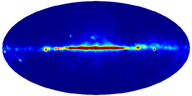
(a) Mollweide projection

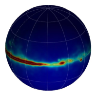
(b) Globe

Figure 5: Full-sky synchrotron map observed by WMAP and smoothed with a Gaussian kernel of ${\rm{FWHM}_{s}}=1.7^{\circ}$. This synchrotron map provides the full-sky background intensity map for our low-resolution simulated observations and is shown here in the global coordinate frame defined by Galactic coordinates.

We simulate observations of the extended source located at $\mbox{\boldmath${\hat{s}}$}_{0}^{{\rm n}}=(\theta_{0}^{\rm n},\varphi_{0}^{\rm n})=(84.0^{\circ},76.5^{\circ})$. In order to compute full-sky visibility contributions, it is necessary to convert the global intensity function to its local coordinate version centred on the interferometer pointing direction. This is performed through a rotation by $\mathcal{R}_{0}^{-1}$ as outlined in Sec. 3.1. The local coordinate intensity function $I^{\rm l}(\mbox{\boldmath${\hat{s}}$}^{{\rm l}})$ is illustrated in Fig. 6 (a). The extended source to be observed is clearly visible at the north pole of this map. The interferometer beam used in these simulations is given by a wide Gaussian with ${\rm FWHM_{b}}\simeq 18^{\circ}$ and is illustrated in Fig. 6 (b).

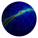
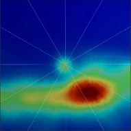
(a) Synchrotron map

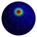
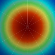
(b) Gaussian beam profile with ${\rm FWHM_{b}}\simeq 18^{\circ}$

Figure 6: Full-sky synchrotron and beam maps in local coordinates. We consider the source at $\mbox{\boldmath${\hat{s}}$}_{0}^{{\rm n}}=(\theta_{0}^{\rm n},\varphi_{0}^{\rm n})=(84.0^{\circ},76.5^{\circ})$. The synchrotron map in global coordinates is rotated by $\mathcal{R}_{0}^{-1}\equiv\mathcal{R}(0,-\theta_{0}^{\rm n},-\varphi_{0}^{\rm n})$ to convert to local coordinates. Full globes are shown on the left; zoomed images of globes about the north pole are shown on the right. Note that the beam profile takes the value of unity in the centre and $\sim\!\!0.3$ at the boundary of the zoomed image.

Given the mock data and configuration discussed previously, we simulate visibilities through direct quadrature on the sphere given by (3.1), the spherical harmonic space representation given by (12) and the SHW space representation given by (16). We assume complete $uv$ coverage and consider a baseline limit of $u_{\rm max}=30$, corresponding to ${\ell_{\rm max}}\simeq 270$, and reconstruct an image of size $N_{\rm image}=20\times 20$. The smoothed synchrotron map is represented by a HEALPix sampled sphere at resolution ${N_{\rm{side}}}=256$ and so is sampled sufficiently for these simulations. Once the visibilities are simulated, a synthesised image is reconstructed simply by taking the inverse Fourier transform. Nyquist sampling dictates that the synthesised image corresponds to a $\sim 20^{\circ}$ square patch. This image reconstruction relies on a tangent plane approximation which will not be valid for the large field of view considered. Nevertheless, this simple approach to reconstruction is sufficient to demonstrate the validity of our full-sky interferometry framework in this restricted low-resolution setting. The application of the standard Fourier transform here to synthesise an image from the simulated visibilities is performed for visual verification only.

The direct projection of the full-sky beam-modulated intensity function onto the tangent plane at the interferometer pointing direction is illustrated in Fig. 7 (a). The images reconstructed from full-sky visibilities computed using all of the methods outlined in Sec. 3 are illustrated in the remaining panels of Fig. 7 (upsampled to a $60\times 60$ pixel image for visualisation). One would expect the tangent plane image of Fig. 7 (a) to differ slightly from the reconstructed images since full-sky contributions due to the large beam are incorporated when simulating visibilities, however a flat-patch approximation is assumed when synthesising the image using the standard Fourier approach. Furthermore, the images synthesised from simulated visibilities contain less high-frequency content as a consequence of the band-limit imposed by the interferometer baseline limit. Nevertheless, all images are in close agreement, demonstrating and validating the use of the methods derived in Sec. 3 to simulate visibilities observed by an interferometer in the full-sky setting. Furthermore, the images contained in panels (b), (c) and (d) of Fig. 7, corresponding respectively to the real, spherical harmonic and naive SHW methods of computing full-sky visibilities are identical (to numerical precision). These images are computed using independent implementations, thereby providing an additional verification of these methods and implementations. In order to realise the advantages of the efficient representation of the SHW basis, it is necessary to ignore near-zero valued wavelet coefficients when computing (16). This is not done in the naive SHW method but strategies to disregard unimportant wavelet coefficients were described in Sec. 3.3.2: constant and annealing based thresholding strategies were proposed. Reconstructed images based on these methods are illustrated in panels (e) and (f) of Fig. 7. These approaches do introduce a small error compared to the images of panels (b) through (d) of Fig. 7, but the controlled introduction of these errors provide substantial computational savings.

   
   

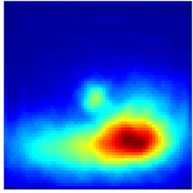
(a) Tangent plane image

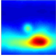
(b) Direct quadrature

(c) Spherical harmonics

(d) Naive SHW

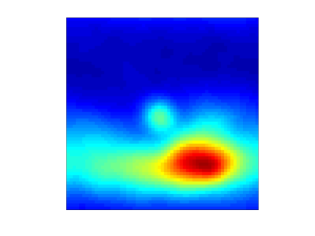
(e) Thresholded SHW (constant threshold)

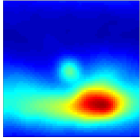
(f) Thresholded SHW (annealing strategy)

Figure 7: Beam-modulated synchrotron intensity images for a $\sim\!\!20^{\circ}$ square patch. The image shown in panel (a) is constructed by projecting the full-sky beam-modulated intensity onto the tangent plane at the interferometer pointing direction defined by the coordinate system $\mbox{\boldmath${p}$}=(p,q)$ (as defined in Sec. 3.1). The images shown in the remaining panels are constructed by simulating visibilities in the full-sky setting using all of the methods described in Sec. 3, followed by a standard inverse Fourier transform to recover the synthesised image. The image in panel (a) is expected to differ to the other images since full-sky contributions due to the large beam are incorporated when simulating visibilities, however a flat-patch approximation is assumed when synthesising images using the standard Fourier approach. Nevertheless, all images are relatively similar, demonstrating and validating the use of the visibility formulations derived in Sec. 3 to simulate visibilities observed by an interferometer in the full-sky setting. The reconstructed images shown in panels (b), (c) and (d) are identical (to numerical precision) as expected, while the reconstructed images shown in panels (e) and (f) differ to these very slightly since some information is discarded when thresholding the wavelet coefficients in order to increase the speed of computations.

In Table 1 we compare the performance of the methods used to compute visibilities in the simulations presented in Fig. 7. The complexity of each method was discussed in Sec. 3 and we collate these complexities here and relate them to the maximum baseline of the interferometer $\|\mbox{\boldmath${u}$}\|_{\rm max}$. For the exact full-sky interferometry formalisms all coefficients are used, be they pixel values, spherical harmonic coefficients or scaling and wavelet coefficients. However, the thresholded SHW strategies require only a small proportion of wavelet coefficients due to the sparse representation of the beam-modulated intensity function in the SHW basis. Typically, less than one percent of the wavelet coefficients can be retained while introducing only minimal errors. It is apparent that the annealed thresholding strategy is slightly superior to the constant thresholding approach, as one would expect since the annealing approach is more likely to retain the detail coefficients of coarser levels that inherently contain more information content. The execution time tests presented in Table 1 show that the thresholded SHW methods are considerably faster than the other methods at this resolution. However, the true advantages of the thresholded SHW methods will only become apparent at higher resolution simulations. At higher resolutions, the real, spherical harmonic and naive SHW methods all scale like $\mathcal{O}(\|\mbox{\boldmath${u}$}\|_{\rm max}{}^{2})$. The already slow performance of these techniques and their poor scaling render these methods computationally infeasible for high-resolution problems. The thresholded SHW methods have much better scaling properties (as discussed in Sec. 3.3.1) and are already considerably faster at this low-resolution, thus rendering high-resolution simulations feasible.

Table 1: Comparison of the performance of the methods derived in Sec. 3 for simulating interferometric observations in the full-sky setting. The results presented in this table correspond to the simulations illustrated in Fig. 7. Execution time tests were performed on a laptop with a 2.2GHz Intel Core 2 Duo processor and 2GB of memory.

Method	Complexity $\mathcal{O}(\|\mbox{\boldmath${u}$}\|_{\rm max}{}^{n})$	Coefficients retained	Execution time
Direct quadrature	$n=2$	100.00%	207.6s
Spherical harmonic	$n=2$	100.00%	263.7s
Naive SHW	$n=2$	100.00%	238.9s
Thresholded SHW (constant threshold)	$n\lesssim 1$	0.70%	75.8s
Thresholded SHW (annealing strategy)	$n\lesssim 1$	0.35%	73.0s

4.3 High-resolution simulated dust observations

In this section we simulate high-resolution observations of Galactic dust emission made by an idealised interferometer. Full-sky visibilities are simulated using the annealing based thresholded SHW method only since computational considerations preclude the application of real and spherical harmonic representations, and the annealing based SHW method was demonstrated in Sec. 4.2 to be superior to the constant thresholding method. We subsequently refer to the annealing based SHW method for simulating full-sky visibilities as the fast SHW method.

The synchrotron map considered previously does not contain enough high-frequency content for the high-resolution simulations performed here. For the background intensity map we therefore use the 94GHz FDS map of predicted submillimeter and microwave emission of diffuse interstellar Galactic dust (Finkbeiner et al., 1999). This predicted map is based on the merged Infrared Astronomy Satellite (IRAS) and Cosmic Background Explorer Diffuse Infrared Background Experiment (COBE-DIRBE) observations produced by Schlegel et al. (1998). An undersampled version of the FDS map is available from LAMBDA as a HEALPix sphere at resolution ${N_{\rm{side}}}=512$. The FDS map that we assume as our full-sky background intensity map $I^{\rm n}(\mbox{\boldmath${\hat{s}}$}^{{\rm n}})$, to be observed by our idealised interferometer, is illustrated in Fig. 8 (a) and (b) in global coordinates. We simulate observations of the extended source located at $\mbox{\boldmath${\hat{s}}$}_{0}^{{\rm n}}=(\theta_{0}^{\rm n},\varphi_{0}^{\rm n})=(108.0^{\circ},0.0^{\circ})$. It is necessary to convert the global intensity function to its local coordinate version through a rotation by $\mathcal{R}_{0}^{-1}$ in order to compute visibilities. The local coordinate intensity function $I^{\rm l}(\mbox{\boldmath${\hat{s}}$}^{{\rm l}})$ is illustrated in Fig. 8 (c) and (d). The extended source to be observed is clearly visible at the north pole of this map. The interferometer beam used in these simulations is given by a Gaussian with ${\rm FWHM_{b}}\simeq 2.9^{\circ}$.

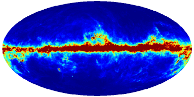
(a) Mollweide projection in global coordinates

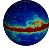
(b) Globe in global coordinates

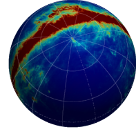
(c) Globe in local coordinates

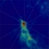
(d) Zoomed globe in local coordinates

Figure 8: Full-sky 94GHz FDS map of predicted submillimeter and microwave emission of diffuse interstellar Galactic dust. This map provides the full-sky background intensity map for our high-resolution simulated observations. Panels (a) and (b) show the full-sky map in the global coordinate frame defined by Galactic coordinates. We simulate observations of the source at $\mbox{\boldmath${\hat{s}}$}_{0}^{{\rm n}}=(\theta_{0}^{\rm n},\varphi_{0}^{\rm n})=(108.0^{\circ},0.0^{\circ})$. A rotation by $\mathcal{R}_{0}^{-1}\equiv\mathcal{R}(0,-\theta_{0}^{\rm n},-\varphi_{0}^{\rm n})$ is performed to convert the map to the local coordinate versions illustrated in panels (c) and (d), which are centred on the north pole.

Given the mock data and configuration discussed above, we simulate visibilities using the fast SHW method (i.e. the annealing based thresholded SHW approach). We assume complete $uv$ coverage and consider a baseline limit of $u_{\rm max}=100$, and reconstruct an image of size $N_{\rm image}=20\times 20$. Following the approach performed in Sec. 4.2, a synthesised image is reconstructed from simulated visibilities simply by taking the inverse Fourier transform. The limitations of this approach were discussed previously, however it is suitable for visual verification of the simulations performed in this article. Nyquist sampling dictates that the synthesised image corresponds to a $\sim 5.7^{\circ}$ square patch.

The direct projection of the full-sky beam-modulated intensity function onto the tangent plane at the interferometer pointing direction is illustrated in Fig. 9 (a). The beam-modulated intensity image reconstructed from the full-sky simulated visibilities is illustrated in Fig. 9 (b) (upsampled to a 60$\times$60 pixel image for visualisation). In this simulation visibilities are computed using 0.023 percent of the wavelet coefficients of the beam-modulated intensity function only. Again, one expects the tangent plane and reconstructed images to differ slightly since full-sky contributions are incorporated when simulating visibilities, however a flat-patch approximation is assumed when synthesising the image using the standard Fourier approach. Furthermore, the fast SHW method itself introduces some small error when discarding those wavelet coefficients with minimal information content and the interferometer baseline limit also restricts the high-frequency content of the reconstructed image. Nevertheless, the tangent plane and reconstructed image are in close agreement, demonstrating and validating the application of the fast SHW approach to simulate full-sky visibilities observed by an interferometer in a high-resolution setting.

The high-resolution simulations performed here using the fast SHW method required an execution time of 289.6s. Based on the scaling relationships of the real and spherical harmonic space methods, and their execution times on the low-resolution simulations performed in Sec. 4.2, we estimate the execution time of these methods when applied to these high-resolution simulations to be $\sim 3000$s. As the resolution of the problem (i.e. the baseline limit $u_{\rm max}$) and the number of visibilities to be computed (i.e. $N_{\rm image}$ in this notation) increase, this difference will become even more marked. The fast SHW method is therefore essential to compute realistic simulations of visibilities when incorporating full-sky contributions. In future, we intend to parallelise our implementation of the fast SHW method and apply it to produce realistic simulations of full-sky interferometer observations, including incomplete $uv$ coverage and other more realistic assumptions.

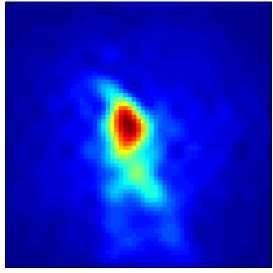
(a) Tangent plane image

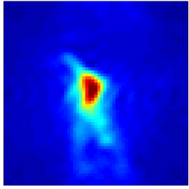
(b) Simulated full-sky interferometric image

Figure 9: Beam-modulated Galactic dust intensity images for a $\sim\!\!5.7^{\circ}$ square patch. The image shown in panel (a) is constructed by projecting the full-sky beam-modulated intensity onto the tangent plane at the interferometer pointing direction defined by the coordinate system $\mbox{\boldmath${p}$}=(p,q)$ (as defined in Sec. 3.1). The image shown in panel (b) is constructed by simulating visibilities in the full-sky setting using the fast SHW method, followed by a standard inverse Fourier transform to recover the synthesised image. The images in panels (a) and (b) are expected to differ since full-sky contributions due to the large beam are incorporated when simulating visibilities, however a flat-patch approximation is assumed when synthesising the image using the standard Fourier approach. Furthermore, the fast SHW method itself introduces some small error when discarding those wavelet coefficients with minimal information content. Nevertheless, the two images are relatively similar, demonstrating and validating the use of the fast SHW method to simulate full-sky visibilities in a high-resolution setting.

5 Conclusions

Next generation interferometers will have very large fields of view, which poses a number of imaging challenges. The usual interferometric approach to simulate visibilities or reconstruct images is based on standard Fourier imaging, which relies on a tangent plane approximation that is valid only for a small field of view. This approach is inappropriate for the wide fields of view proposed for the next generation of interferometers. In this article we have formulated interferometry in the full-sky setting, incorporating contributions over the entire sky to ensure that contamination due to wide sidelobes of primary beams is not neglected. Full-sky interferometry formulations have been developed in real, spherical harmonic and SHW spaces. The SHW formulation proves the most advantageous approach due to the efficient representation of the spatially localised high-frequency content typical of primary beams and sky intensity functions in the wavelet basis. A corresponding fast SHW method was developed to simulate full-sky visibilities. The fast SHW method exploits the sparsity of the wavelet representation by discarding all wavelet coefficients that contain minimal information content. A quadratic annealing based thresholding strategy was developed to determine those wavelet coefficients that may be safely discarded. The resulting fast SHW method has superior computational scaling properties and may be performed at a substantially lower computational cost than the real and spherical harmonic space methods for simulating visibilities when including full-sky contributions.

The primary focus of this article is the use of these full-sky interferometry representations to simulate visibilities, however we also briefly discussed implications for the reconstruction of images on wide fields of view. Although it is possible in theory to reconstruct full-sky images in the spherical harmonic representation, this requires full sampling of the visibility function in $\mathbb{R}^{3}$ and hence is not likely to be well posed in practice. However, image reconstruction on wide fields of view is likely to be well posed in SHW space and we outlined a preliminary method to perform wide field image reconstruction. The use of SHWs for image reconstruction is an interesting application in its own right and we intend to develop these ideas further and to evaluate their effectiveness in a future work.

To demonstrate the application of our full-sky interferometry representations for simulating visibilities, and to compare the various methods, we simulated low-resolution full-sky interferometric observations of synchrotron emission using all of the methods. The real, spherical harmonic and naive SHW methods recovered identical images of the extended source observed by our idealised interferometer, where the naive SHW method does not exploit sparse representations in the wavelet basis. The fast SHW method does exploit sparse representations, introducing a small error when discarding those wavelet coefficients that contain minimal information content, but consequently the speed of computations in increased substantially. Typically less than one percent of wavelet coefficients are retained in these low-resolution simulations, reducing the execution time of simulations by a factor of approximately three compared to the other methods (while introducing only minimal errors in reconstructed images). However, the true advantages of the fast SHW method only become apparent on high-resolution simulations due to its superior scaling properties.

The already slow performance of the real and spherical harmonic space approaches to simulating full-sky visibilities, and their poor scaling properties, render these methods computationally infeasible on higher resolution problems. Computing full-sky visibilities using the fast SHW method adapts to the extremely sparse representation of the beam and sky intensity function in the wavelet basis, thus easing the computational burden of simulations to the extent that they are rendered computationally feasible at high-resolutions. Using this method high-resolution interferometric observations of diffuse interstellar Galactic dust were simulated, demonstrating and validating the use of the fast SHW method for simulating visibilities in a high-resolution setting. In this example only 0.023 percent of wavelet coefficients were retained and the execution time of simulations was estimated to be greater than an order of magnitude faster than simulations based on the real or spherical harmonic space full-sky interferometry formulations.

Now that it is possible to simulate the visibilities observed by an interferometer when including contributions over the entire sky, a number of related studies may be performed. Firstly, we intend to parallelise our implementations and develop more realistic simulations of full-sky interferometer observations, including incomplete $uv$ coverage and other more realistic assumptions. Using these simulations, we then intend to study the effect of contamination in realistic interferometric observations due to wide sidelobes of primary beams. Secondly, our full-sky interferometry formulation allows one to simulate visibilities for all values of $\mbox{\boldmath${u}$}=(u,v,w)$, and not only values of ${u}$ where $w=0$, as is the case with the standard Fourier transform approach. Such simulations allow one to evaluate the performance of the faceting (Cornwell & Perley, 1992; Greisen, 2002) and $w$-projection (Cornwell et al., 2005) approaches to wide field image reconstruction on simulations where the ground truth is known. Thirdly, we have highlighted an interesting alternative approach to wide field image reconstruction based on the SHW representation that warrants further study. We intend to pursue all three of these applications in future work. The ability to perform realistic high-resolution simulations of interferometric observations that include full-sky contributions, afforded by our fast SHW formulation, allows many new studies to be performed that will be important to the design of next generation interferometers and to the development of algorithms to analyse the data generated by these instruments.

References

- Antoine et al. (2002) Antoine J.P., Demanet L., Jacques L., Vandergheynst P., 2002, Applied Comput. Harm. Anal., 13, 3, 177
- Antoine et al. (2004) Antoine J.P., Murenzi R., Vandergheynst P., Ali S.T., 2004, Two-Dimensional Wavelets and their Relatives, Cambridge University Press, Cambridge
- Antoine & Vandergheynst (1998) Antoine J.P., Vandergheynst P., 1998, J. Math. Phys., 39, 8, 3987
- Antoine & Vandergheynst (1999) Antoine J.P., Vandergheynst P., 1999, Applied Comput. Harm. Anal., 7, 1
- Barreiro et al. (2000) Barreiro R.B., Hobson M.P., Lasenby A.N., Banday A.J., Górski K.M., Hinshaw G., 2000, Mon. Not. Roy. Astron. Soc., 318, 475, astro-ph/0004202
- Bogdanova et al. (2005) Bogdanova I., Vandergheynst P., Antoine J.P., Jacques L., Morvidone M., 2005, Applied Comput. Harm. Anal., 19, 2, 223
- Brink & Satchler (1999) Brink D.M., Satchler G.R., 1999, Angular Momentum, Clarendon Press, Oxford, 3rd edition
- Bunn & White (2007) Bunn E.F., White M., 2007, Astrophys. J., 655, 21, astro-ph/0606454
- Cornwell et al. (2005) Cornwell T.J., Golap K., Bhatnagar S., 2005, in N. Kassim, M. Perez, W. Junor, P. Henning, editors, Astronomical Data Analysis Software and Systems XIV, volume 345 of Astronomical Society of the Pacific Conference Series, 350–+
- Cornwell & Perley (1992) Cornwell T.J., Perley R.A., 1992, Astron. & Astrophys., 261, 353
- Dahlke & Maass (1996) Dahlke S., Maass P., 1996, J. Fourier Anal. and Appl., 2, 379
- Daubechies (1992) Daubechies I., 1992, Ten Lectures on Wavelets, CBMS-NSF Reg. Conf. Series in Applied Math., SIAM, Philadelphia
- Demanet & Vandergheynst (2003) Demanet L., Vandergheynst P., 2003, in Proc. SPIE, volume 5207, 208–215
- Driscoll & Healy (1994) Driscoll J.R., Healy D.M.J., 1994, Advances in Applied Mathematics, 15, 202
- Finkbeiner et al. (1999) Finkbeiner D.P., Davis M., Schlegel D.J., 1999, Astrophys. J., 524, 867, astro-ph/9905128
- Freeden et al. (1997) Freeden W., Gervens T., Schreiner M., 1997, Constructive approximation on the sphere: with application to geomathematics, Clarendon Press, Oxford
- Freeden & Windheuser (1997) Freeden W., Windheuser U., 1997, Applied Comput. Harm. Anal., 4, 1
- Górski et al. (2005) Górski K.M., Hivon E., Banday A.J., Wandelt B.D., Hansen F.K., Reinecke M., Bartelmann M., 2005, Astrophys. J., 622, 759, astro-ph/0409513
- Greisen (2002) Greisen E., 2002, in URSI General Assembly
- Hinshaw et al. (2007) Hinshaw G., et al., 2007, Astrophys. J. Supp., 170, 288, astro-ph/0603451
- Hobson & Magueijo (1996) Hobson M.P., Magueijo J., 1996, Mon. Not. Roy. Astron. Soc., 283, 1133, astro-ph/9603064
- Holschneider (1996) Holschneider M., 1996, J. Math. Phys., 37, 4156
- Liu & Zou (2007) Liu H., Zou J., 2007, IMA J. Appl. Maths, 72, 6, 817
- McEwen et al. (2006) McEwen J.D., Hobson M.P., Lasenby A.N., 2006, ArXiv, astro-ph/0609159
- Ng (2001) Ng K.W., 2001, Phys. Rev. D., 63, 12, 123001, astro-ph/0009277
- Ng (2005) Ng K.W., 2005, Phys. Rev. D., 71, 8, 083009, astro-ph/0409007
- Risbo (1996) Risbo T., 1996, J. Geodesy, 70, 7, 383
- Sanz et al. (2006) Sanz J.L., Herranz D., López-Caniego M., Argüeso F., 2006, in EUSIPCO, astro-ph/0609351
- Schlegel et al. (1998) Schlegel D.J., Finkbeiner D.P., Davis M., 1998, Astrophys. J., 500, 525, astro-ph/9710327
- Schröder & Sweldens (1995) Schröder P., Sweldens W., 1995, in Computer Graphics Proceedings (SIGGRAPH ‘95), 161–172
- Starck et al. (2006) Starck J.L., Moudden Y., Abrial P., Nguyen M., 2006, Astron. & Astrophys., 446, 1191, astro-ph/0509883
- Sweldens (1996) Sweldens W., 1996, Applied Comput. Harm. Anal., 3, 2, 186
- Sweldens (1997) Sweldens W., 1997, SIAM J. Math. Anal., 29, 2, 511
- Tenorio et al. (1999) Tenorio L., Jaffe A.H., Hanany S., Lineweaver C.H., 1999, Mon. Not. Roy. Astron. Soc., 310, 823, astro-ph/9903206
- Thompson et al. (2001) Thompson A.R., Moran J.M., Jr. G.W.S., 2001, Interferometry and synthesis in radio astronomy, Wiley-VCH, Weinheim, 2nd edition
- Torrésani (1995) Torrésani B., 1995, Signal Proc., 43, 341
- Varshalovich et al. (1989) Varshalovich D.A., Moskalev A.N., Khersonskii V.K., 1989, Quantum theory of angular momentum, World Scientific, Singapore
- White et al. (1999) White M., Carlstrom J.E., Dragovan M., Holzapfel W.L., 1999, Astrophys. J., 514, 12, astro-ph/9712195
- Wiaux et al. (2005) Wiaux Y., Jacques L., Vandergheynst P., 2005, Astrophys. J., 632, 15, astro-ph/0502486
- Wiaux et al. (2008) Wiaux Y., McEwen J.D., Vandergheynst P., Blanc O., 2008, Mon. Not. Roy. Astron. Soc., 388, 2, 770, arXiv:0712.3519