Neutrino Signals from Solar Neutralino Annihilations in Anomaly Mediated Supersymmetry Breaking Model

Abstract

The lightest neutralino, as the dark matter candidate, can be gravitationally captured by the Sun. In this paper, we studied the high energy neutrino signals from solar neutralino annihilations in the core of the Sun in the anomaly mediated supersymmetry (SUSY) breaking (AMSB) model. Based on the event-by-event monte carlo simulation code WimpSim, we studied the detailed energy and angular spectrum of the final muons at large neutrino telescope IceCube. More precisely we simulated the processes since the production of neutrino via neutralino annihilation in the core of the Sun, neutrino propagation from the Sun to the Earth, as well as the converting processes from neutrino to muon. Our results showed that in the AMSB model it is possible to observe the energetic muons at IceCube, provided that the lightest neutralio has relatively large higgsino component, as a rule of thumb $N_{13}^{2}+N_{14}^{2}>4\%$ or equivalently $\sigma_{SD}>10^{-5}pb$. Especially, for our favorable parameters the signal annual events can reach 102 and the statistical significance can reach more than 20. We pointed out that the energy spectrum of muons may be used to distinguish among the AMSB model and other SUSY breaking scenarios.

I Introduction

Over the past several years, the picture that our universe is not baryon dominant is well established. Based on the observations of Wilkinson Microwave Anisotropy Probe (WAMP) and other experiments, the relic dark matter density is fixed to be $0.085<\Omega_{DM}h^{2}<0.119$ within $2\sigma$ uncertainty WMAP . In order to account for the dark matter, physics beyond the standard model (SM) is usually required. Among these new physics the weakly interacting massive particle (WIMP) is one of the popular candidate for the dark matter. One possible WIMP is the lightest supersymmetric (SUSY) particle (LSP) in SUSY theory with R-parity conservation JKG95BHS04 . Usually there are three possible LSPs, namely sneutrino, gravitino and neutralino. The lightest sneutrino has been largely ruled out by direct searches sneutrino , and the gravitino is difficult to be detected due to its very weak interactions with ordinary matter FRT03 . Thus the lightest neutralino, which is combination of gaugino and higgsino, is the most well-motivated candidate for dark matter neutralino .

SUSY breaking mechanism plays an important role to investigate the nature of dark matter. Firstly, in order to be consistent with experimental observations, SUSY must be broken at weak scale. As a consequence, the mass of dark matter is partially determined by the breaking terms. Secondly, we need higher scale SUSY breaking mechanism to reduce the number of free parameters at low energy. As an example there are more than 100 parameters in minimal supersymmetric standard model(MSSM). Thirdly, the properties of the LSP depend on the details of SUSY breaking mechanism. For example in minimal supergravity (mSUGRA) model, the main component of the lightest neutralino can be the bino in ’bulk region’, while in ’focus point region’, the lightest neutralino can have larger higgsino content CCN98 ; FMM ; FW05 ; BKPU05 ; FMW . Here ’bulk region’ and ’focus point region’ are determined by different SUSY breaking parameters. Thus it is interesting to explore (i) the predictions for different SUSY breaking mechanisms; and (ii) whether the detection of dark matter can distinguish among the different SUSY breaking mechanisms.

While in literature the mSUGRA model was widely investigated, in this paper we are interested in the properties of neutralino (as the dark matter particle) and its detection in the scenario of the anomaly mediated SUSY breaking (AMSB)RS98 ; GLMR98 . Many predictions in AMSB models are different from those in usual mSUGRA models and other SUSY breaking scenarios. One feature of AMSB model is the special gaugino mass relation calculated by $\beta$ function, $M_{1}:M_{2}:|M_{3}|=2.8:1:7.1$ GGW99 , which implies that the lightest chargino pair and neutralino comprise a nearly mass-degenerate triplet of winos over most of the MSSM parameter space. Moreover the lightest neutralino is mostly wino-like. Such kind of neutralino usually has larger cross section compared to that in mSUGRA model. As a consequence, if it is the dark matter, it should be produced in non-thermal processes GGW99 ; MR99 , or should be very heavy, generally larger than $2\ TeV$ W04 ; CDKR06 ; HMNSS06 .

The methods to detect dark matter can be classified into direct and indirect ones. The former methods detect dark matter by measuring the recoil of nucleus. The latter ones detect the final stable particles, including neutrinos, antiprotons, positrons, antinuclei and photons, which are produced by dark matter annihilation. In this paper we will focus on the observation by neutrino telescopes which detect the high energy neutrinos from dark matter annihilations (for some recent works, see FMW ; highE ; BKS01BDK02 ; BHHK02 ; HK02 ; HS05 ; iceneutrino ; LE04 ; CFMSSV05 ; BKST07 ; LW07 ). The non-relativistic dark matter would be trapped by Sun or Earth via gravitational force. The captured dark matter can annihilate into SM particles, including neutrinos, in the center of Sun or EarthPS85 ; neutrino ; earlywork . The resulting neutrinos interact with usual matter feebly, thus it is possible for us to detect them after a long propagation. Many neutrino telescopes for high energy neutrino have been built or are under construction such as IceCube icecube ; Aetal04 , Super-Kamiokande superk , AMANDA amanda and ANTARES antares etc. In this paper we will focus on the neutrino detection at IceCube. The IceCube detector now is being built in the south pole and will be completed in 2010 icecube ; Aetal04 . The scale of the IceCube is in square kilometers and it can detect neutrinos with threshold energy of $50\ GeV$icecube .

In this paper, we will discuss neutrino signals from neutralino annihilations in the Sun in AMSB scenario. The final muon events rate at the IceCube detector can be determined by E93 :

$$\Gamma_{events}=\Gamma_{ann}A_{eff}\sum_{i}Br_{i}\Phi_{\mu i}$$ (1)

where $\Gamma_{ann}$ is neutralino’s annihilation rate in the Sun, $A_{eff}$ is detector’s actual effective detected area, $Br_{i}$ is the branching fraction of i-th annihilation channel, and $\Phi_{\mu}$ is the $\mu$ flux over detector threshold per unit area and parent pair. Our study shows that for the Sun there exit the parameter space which can induce the large neutralino capture rate and thus the large neutralino annihilation rate $\Gamma_{ann}$. In this case, most neutrinos come from $W$ decay and the $W$s are pair produced via neutralino annihilations. Such neutralino is wino-like. Recently the authors of Ref. BKST07 pointed out that if the spin effects of neutralino annihilation are included, the energy spectrum of neutrinos in the Sun will be different. Thus in our study we include such kind of spin effects. We utilize Calchep comphep ; calchep to generate events of neutralino annihilation based on exact matrix elements calculation. We then import these events into Monte Carlo simulation program - WimpSim wimpsim which performs a thorough analysis for neutrinos propagation from the Sun to detector at the surface of the Earth BEO07 . The program contains some important features similar to those of Pythia pythia , Darksusy darksusy and nusigma nusigma . Thus WimpSim can analyze details of neutrino propagation and detection including both neutrino oscillations and interactions BEG ; E93 ; E97 ; BEO07 . The detail Monte Carlo simulations allow us tracing every neutrino event and determining final $\mu$ signals with the concrete energy and angle information. At the same time, we will consider the real environment of IceCube detector Aetal04 ; GHM05 , and obtain the realistic final muon spectrum.

This paper is organized as following. In section II we will briefly discuss some features of AMSB model and the properties of the neutralino. In section III, we perform the parameter space scan to determine different neutralino capture rates for the Sun. In section IV, we explore all important neutralino annihilation channels, then calculate the spectrum of neutrinos from the production of neutralino annihilation. In section V, we investigate the propagation of neutrinos from center of the Sun to the Earth. In section VI, the final spectrum of $\mu$ is presented. The last section contains our conclusions and discussions.

II Neutralino in the AMSB model

Anomaly-mediated contributions to SUSY breaking usually appear in supergravity theory, but they are loop suppressed compared to those of gravity-mediated. However the latter contributions are assumed to be zero in the AMSB scenario. In this scenario there are no direct interaction between hidden and visible sectors RS98 ; GLMR98 . Thus the masses of neutralino and slepton are zero at tree level. The soft SUSY breaking terms are related to the super-conformal anomaly, and they appear at loop level. In the hidden sector, an auxiliary field as a super-gravity ground can be thought as the only origin to break SUSY. In order to have a conformal lagrangian, a compensator superfield $\phi$ is introduced RS98 ; GLMR98 ; PR99 . We can assume that $\phi$ get non zero value as

$$\phi=1+<F_{\phi}>\theta^{2},$$ (2)

then expand $\phi$ in background value $<F_{\phi}>=-m_{3/2}$ ($m_{3/2}$ is related to the mass of gravitino) and perform calculation with re-scaling the coupling of matter field. The soft SUSY breaking terms related to gauginos and sleptons are calculated to be GGW99 :

$$M_{\lambda} = \frac{\beta_{g}}{g}m_{3/2}$$ (3)

$$m_{\bar{Q}}^{2} = -\frac{1}{4}(\frac{\partial\gamma}{\partial g}\beta_{g}+\frac{\partial\gamma}{\partial y}\gamma_{y})m_{3/2}^{2}$$ (4)

$$A_{y} = -\frac{\beta_{y}}{y}m_{3/2},$$ (5)

where $\gamma$, $\beta$ are functions defined as

$$\gamma\equiv\frac{d\ln Z}{d\ln\mu},\,\,\,\beta_{g}\equiv\frac{dg}{d\ln\mu},\,\,\,\beta_{y}\equiv\frac{dy}{d\ln\mu}.$$ (6)

From these formulas we can see that the masses of SUSY particles in AMSB scenario are determined by $m_{3/2}$ and evolutions of gauge and Yukawa couplings. It is interesting to note that the mass of slepton in the Eqn.(4) is negative. In literature several solutions are proposed PR99 ; KK00 ; CL01 ; MSS08 . Phenomenologically one can simply add a universal positive mass terms $m_{0}^{2}$ to the right hand of Eqn.(4) GGW99 ; FM99 . The resulting model is dubbed as minimal AMSB (mAMSB) model which only depends on

$$m_{3/2},\,m_{0},\,\tan\beta,\,sign(\mu)$$ (7)

as the extra free parameters.

The mAMSB model is highly predictive. One of the important predictions is the relationship between gaugino masses as $M_{1}:M_{2}:|M_{3}|=2.8:1:7.1$ at the low energy scale, which implies that the lightest neutralino is mostly wino-like over most of the MSSM parameter space. It is known that in MSSM the neutralino is a linear combination of gauginos and higgsinos, and the lightest neutralino is given as

$${\widetilde{\chi}_{1}^{0}}=N_{11}\tilde{B}+N_{12}\tilde{W}+N_{13}\tilde{H_{d}}+N_{14}\tilde{H_{u}}.$$ (8)

On the contrary the lightest one is bino-like over most of the mSUGRA parameter space with GUT assumption.

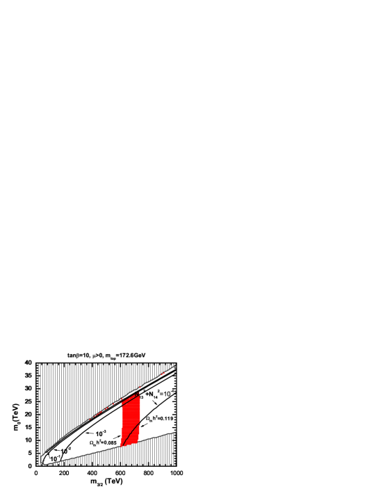
Figure 1: The allowed points which can induce correct thermal relic density $0.085<\Omega_{th}h^{2}<0.119$ in the plane of $m_{3/2}$ and $m_{0}$. Curves of $N_{13}^{2}+N_{14}^{2}$ (as a measure for the lightest neutralino Higgsino components) are also shown. The left-top region is excluded because it can not radiatively lead to EWSB, and the right-bottom region is excluded because it has tachyon. The allowed points are generated by MicrOMEGAs micromegas .

In Fig. 1 we show the points which can result in the correct thermal relic density in $m_{3/2}$ and $m_{0}$ plane. We utilize Suspect code suspect to scan parameter space in mAMSB model. For the case of $N_{13}^{2}+N_{14}^{2}\lesssim 0.1$, the relic density can be approximately given as GR04

$$\Omega_{th}h^{2}\simeq 0.02(\frac{M_{2}}{1TeV})^{2}.$$ (9)

Such kind of lightest neutralinos usually has large annihilation cross sections in the thermodynamic equilibrium of early universe, therefore it is not easy to induce the correct relic density. However one can still obtain the correct density if lifting the mass of neutralino to be as heavy as $1.9\sim 2.3$ TeV CDKR06 ; W04 . If wino-like neutralino with $SU(2)_{L}$ charge is much heavier than the weak gauge boson, the weak interaction is a long-distance force for non-relativistic two-bodies states of such particles. If this non-perturbative effect (namely Sommerfeld enhancement) of the dark matter at the freeze-out temperature is taken into account, the abundance can be reduced by $\sim 50\%$. Thus the neutralino mass would be as heavy as $2.7\sim 3.0$ TeVHMNSS06 . Such heavy neutralino may be detected through dark matter search experiments CDKR06 ; HMNS0412 ; HMSS05 , but it is difficult to detect and study it at the LHC and the planning ILC. For the case of $N_{13}^{2}+N_{14}^{2}>0.1$, the light neutralino can also induce the correct density for a tiny region of parameter space, which lies in the vicinity of boundary of the electroweak symmetry breaking (EWSB). Here the $|\mu|$ decreases and Higgsino components become significant.

Now that the light neutralino hardly accounts for thermal relic density in the mAMSB model, another approach is proposed, i.e. the neutralino is not mainly from thermal production. Some authors discussed the mechanism that the LSP is produced by the decay of gravitinos GGW99 ; MR99 (or moduli fields MR99 ) in the AMSB model. From Eqn.(3) we can see that neutralino is much lighter than that of gravitino. If the gravitinos have a relatively short lifetime, this mechanism will not destroy the success of big-bang nucleosynthesis (BBN) MR99 . In this scenario, the light LSP with large wino component can be the good candidate for dark matter. However it should be pointed out that although this kind of LSP with large cross section could be produced in non-thermal process, it is also constrained by cosmological observations. For example, in the center of our galaxy, we may observe the signals of the dark matter annihilation BE98HS04PU04 ; HD02 ; YHBA07 due to their large cross sections. Recently, Ref. H08 reported that if assuming an excess of microwave emission in the inner Milky Way is due to dark matter annihilation, the synchrotron measurements give constraint to the annihilation rate of neutralino. The constraint depends on the dark matter distribution profile. More stringent constraint has been reported by Ref. J04 . The residual annihilation of dark matter would produce ⁶Li during the BBN. Then the observations of abundance of ⁶Li could constrain the dark matter annihilation rate. The low mass wino-like dark matter below $250$ GeV in AMSB model has been ruled out J04 . It is still possible to detect heavier wino-like neutralino at the high energy collider detamsbcol and non-accelerator dark matter search experiments MR99 ; U01 ; HW04 ; HMNS0407 .

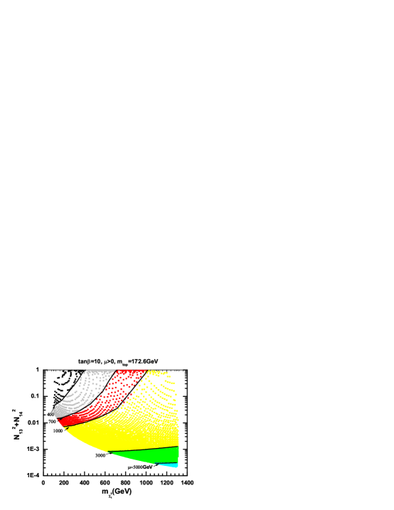
Figure 2: Points which can induce relic density lower than 0.119 in the plane of lightest neutralino mass and $N_{13}^{2}+N_{14}^{2}$. Here $0<m_{0}<20TeV$ and $0<m_{3/2}<400TeV$. The curves with different $\mu$ at 5000, 3000, 1000, 700, 400 GeV are also plotted. We can see that the light neutralino with small $\mu$ is easy to get large Higgsino component.

The general relation between $\mu$ and other parameters in SUSY at tree level is given by

$$\mu^{2}=\frac{m_{H_{d}}^{2}-m_{H_{u}}^{2}\tan^{2}\beta}{\tan^{2}\beta-1}-\frac{1}{2}m_{Z}^{2}.$$ (10)

As discussion in Ref. FM99 , pure anomaly-mediated value of $m_{H_{u}}^{2}$ is renormaliztion group (RG) invariant, and non anomaly-mediated contribution of $\delta m_{H_{u}}^{2}$ would be even zero for some parameters. This focusing behavior near the weak scale makes $m_{H_{u}}^{2}$ only lightly dependent on ultra-violet (UV) boundary and would give suitable small $\mu$ for naturalness requirement. At the same time it will lead to considerable higgsino component of the LSP, which is similar as that in ’focus point region’ in mSUGRA model CCN98 ; FMM ; FW05 ; BKPU05 ; FMW . In Fig. 1 and Fig. 2, the parameter scan was done by using MicrOMEGAs micromegas and Suspectsuspect with parameters $\tan\beta=10,\mu>0,m_{top}=172.6GeV$ CDFD0 . In Fig.1, the left-top region is excluded because the radiative EWSB condition fails. With the decrement of $|\mu|$, the Higgsino composition becomes larger near the boundary. In this parameter region, the lightest neutralino could be partially non-thermal-produced. At the same time, some points can even directly satisfy thermal relic density due to relative small wino content. In Fig. 2 we show the points which can induce relic density lower than 0.119 in the plane of $m_{\tilde{\chi}_{1}^{0}}$ and $N_{13}^{2}+N_{14}^{2}$. Here we choose $0<m_{0}<20$ TeV and $0<m_{3/2}<400$ TeV, which is smaller than those in Fig. 1. The reason is that the heavy neutralino, which corresponds to large $m_{0}$ and $m_{3/2}$, usually have small spin-dependent cross-section $\sigma_{SD}$ (see Fig. 4 below), consequently low capture rate in the Sun. We impose the constraints as $m_{h}>114.4GeV$ ADLO03 , relic density $\Omega h^{2}<0.119$ WMAP , $\Delta\rho<2\times 10^{-3}$, $B(b\to s\gamma)=(355\pm 26)\times 10^{-6}$HFAG and $\Delta a_{\mu}(Exp-SM)=(26.1\pm 9.4)\times 10^{-10}$ g-2 within $3\sigma$ uncertainty. Note that in scattered plots in Fig. 3, Fig. 4 and Fig. 5, we also choose $0<m_{0}<20TeV$, $0<m_{3/2}<400TeV$ and with the same parameters and constraints as in Fig. 2. In our chosen parameter space, the relic density is well under upper limit of WMAP. A few words on the constraint from $a_{\mu}$ is worth to mention. Recently, the authors of Ref. HMNT07 updated SM prediction of $a_{\mu}$ which has a smaller uncertainty and corresponds to a $3.4\sigma$ deviation from the measured value in Ref. g-2 . In mAMSB model, parameter space with large $m_{0}$ and $m_{3/2}$ is heavily constrained because the SUSY contributions are suppressed by heavy superparticle masses. In mSUGRA model, for the same reason the parameter space with large $m_{0}$ and $m_{1/2}$ is also severely constrained.

III Capture and annihilation rate of dark matter in the AMSB model

There are dark matter in our galactic halo, and the dark matter particles will scatter off nucleus in astrophysical objects such as the Sun and the Earth and be gravitationally trapped in them PS85 . Once captured, dark matter particles will have a larger annihilation rate due to the larger density and will produce the energetic SM particles. These SM particles are mostly absorbed by the matter except neutrinos which interact feebly with ordinary matter. The evolution of dark matter number in the objects can be written as

$$\dot{N}=C_{\odot}-C_{A}N^{2}.$$ (11)

Here $C_{\odot}$ is the capture rate and $C_{A}\equiv<\sigma v>/V_{eff}$ is thermally averaged annihilation cross section per volume. The annihilation rate can be solved as

$$\Gamma=\frac{1}{2}C_{A}N^{2}=\frac{1}{2}C_{\odot}\tanh^{2}(\sqrt{C_{\odot}C_{A}}t),$$ (12)

where $t$ is the age of this system and $\frac{1}{2}$ is due to the two LSPs annihilation. For the Sun, $\sqrt{C_{\odot}C_{A}}t\gg 1$ leads an approximation of above result as $\Gamma=\frac{1}{2}C_{\odot}$. The capture rate for the Sun is then given as G92

$$C_{\odot}=3.4\times 10^{20}s^{-1}\frac{{\rho_{local}}}{{0.3GeV/cm^{3}}}(\frac{{270km/s}}{{v_{local}}})(\frac{{\sigma_{SD}^{H}+\sigma_{SI}^{H}+0.07\sigma_{SI}^{He}}}{{10^{-6}pb}})(\frac{{100GeV}}{{m_{\widetilde{\chi}_{1}^{0}}}})^{2},$$ (13)

where $\rho_{local}$ is the local mass density of dark matter, and $v_{local}$ is velocity of these particles. In our numerical evaluation we adopt the values $\rho_{local}=0.3\ GeV/cm^{3}$ and $v_{local}=220\ km/s$ PDG . Here $\sigma_{SD}$ and $\sigma_{SI}$ are spin-dependent and spin-independent scattering cross sections of LSP with nucleus respectively.

In the capture process, LSPs lose their energy by scattering off the nucleus in the Sun and then trapped by gravity. The capture rate depends on the scattering cross section of LSP with nucleus. The spin-independent scattering cross section $\sigma_{SI}$ has been strictly constrained by direct detection on the Earth. For example XENON10 set an upper limit for the WIMP-nucleon spin-independent cross section of $8.8\times 10^{-8}pb$ for a WIMP mass of $100GeV$, and $4.5\times 10^{-8}pb$ for a WIMP mass of $30GeV$ at 90% confidence level AA08 .

The cross section for scattering of a neutralino off of a proton via spin-dependent interaction is K91 ; RABGMR93 ,

$$\sigma_{SD}=\frac{{32m_{\widetilde{\chi}_{0}^{1}}^{2}m_{p}^{2}G_{F}^{2}}}{{\pi(m_{\widetilde{\chi}_{0}^{1}}+m_{p})^{2}}}J(J+1)[\sum\limits_{u,d,s}{A^{\prime}_{q}\Delta q}]^{2},$$ (14)

where

$$A^{\prime}_{q} = \frac{1}{2}T_{3L}^{q}\left(|N_{13}|^{2}-|N_{14}|^{2}\right)$$ (15)

$$-\frac{{m_{W}^{2}}}{{m_{\widetilde{\chi}_{0}^{1}}^{2}-m_{\widetilde{q}}^{2}}}\left\{\frac{{m_{q}^{2}d_{q}^{2}}}{{2m_{W}^{2}}}+\left[T_{3L}^{q}N_{12}-\tan\theta_{W}(T_{3L}^{q}-e_{q})N_{11}\right]^{2}+\tan^{2}\theta_{W}e_{q}^{2}N_{11}^{2}\right\}.$$

Here $m_{q}$ is the quark mass, $d_{q}=-N_{13}/\cos\beta$ for down-type quarks, $d_{q}=-N_{14}/\sin\beta$ for up-type quarks, $T_{3L}^{q}$ is the weak isospin of the quark and $e_{q}$ is quark electric charge. The quantity $\Delta q$ measures the fraction of the nucleon spin carried by the quark. The values are taken as $\Delta u=0.78$, $\Delta d=-0.5$ and $\Delta s=-0.16$ K91 ; RABGMR93 ; EK93 ; BB98 . The first part of the Eqn. 15 corresponds to the process of exchanging Z boson, and the second part of exchanging squark. For heavy squark, the second term can be safely neglected.

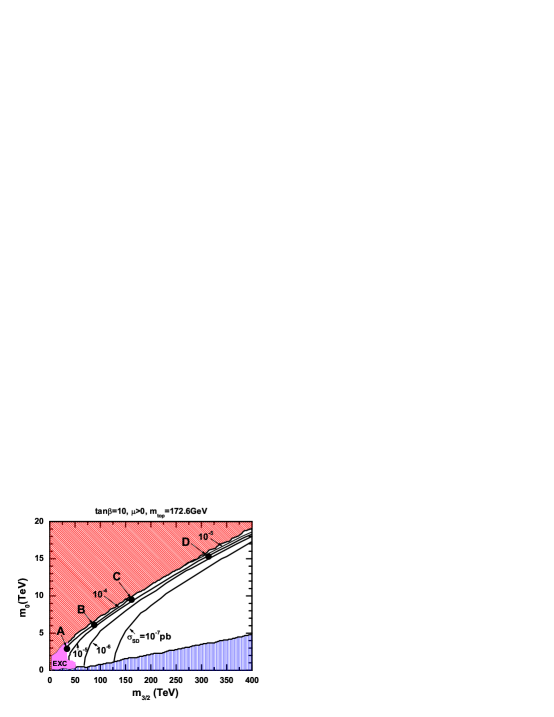
Figure 3: Contours of $\sigma_{SD}$ in the ($m_{3/2},m_{0}$) plane. The constraints are the same as those in Fig. 2. Four benchmark points A, B, C and D, which are used in Tab. 1 and Tab. 2, are also depicted.

Figure 4: Allowed parameter points in the plane of lightest neutralino mass and $\sigma_{SD}$. The parameters $\tan\beta,sign(\mu),m_{top}$ are the same as those in Fig. 3. The constraints are the same as those in Fig. 2.

The cross sections of $\sigma_{SD}$ in AMSB model are plotted in Fig. 3 and Fig. 4. In these two figures the largest neutralino mass is $1.1TeV$. For heavier neutralino the capture rate is rather low because $\sigma_{SD}$ is smaller and it is also suppressed by its mass. In Fig. 4, the $\sigma_{SD}$ varies from $10^{-9}pb$ to $10^{-3}pb$. Note that in Fig. 3 the lightest neutralino, which lies in the vicinity of EWSB boundary, has higher higgsino fraction thus larger cross section $\sigma_{SD}$. In Fig. 3, the lower left portion is excluded by direct accelerator limits on sparticle masses, light Higgs mass constraint.

IV Production and propagation of neutrinos

IV.1 Production of neutrinos in the Sun

The dark matter annihilation in the Sun is calculated in the static limit, i.e. the dark matter is assumed to be at rest, because the velocity of these particles is about $220km/s$ PDG in the solar system. The neutrinos can be directly produced from the lightest neutralinos $\widetilde{\chi}_{0}^{1}$ annihilation. However the neutrino flux is usually negligible compared to those from $\widetilde{\chi}_{0}^{1}$ annihilation to $W^{+}W^{-},ZZ,Zh,f\overline{f}$. In this paper the direct neutrino production from $\widetilde{\chi}_{0}^{1}$ annihilation is not included. In mSUGRA model, usually contributions from each channel to neutrino flux play the same important role. However in AMSB model, $\widetilde{\chi}_{0}^{1}$s mainly annihilate to $W^{+}W^{-}$ which is usually 10-1000 times greater than other modes. The reason is that $\widetilde{\chi}_{0}^{1}$ is mostly constituted by wino and chargino is also composed nearly of charged wino, thus the coupling $W\widetilde{\chi}_{1}^{0}\widetilde{\chi}_{1}^{\pm}$ is much larger than that of $Z\widetilde{\chi}_{1}^{0}\widetilde{\chi}_{1}^{0}$. Note that annihilation rate of the latter one is proportional to $\left|{N_{14}}\right|^{2}-\left|{N_{13}}\right|^{2}$. In Fig. 2, we have shown that $\left|{N_{14}}\right|^{2}+\left|{N_{13}}\right|^{2}$ is small over most of the parameter space, thus the coupling $Z\widetilde{\chi}_{1}^{0}\widetilde{\chi}_{1}^{0}$ is usually small. Especially in the vicinity of EWSB boundary, in which $\widetilde{\chi}_{0}^{1}$ can have large component of Higgsino, the fraction of $\widetilde{\chi}_{0}^{1}$ annihilation to $W^{+}W^{-}$ is always much more larger than $90\%$. In Fig. 5, the fractions of channel $W^{+}W^{-},ZZ,Zh,t\overline{t}$ are plotted. From the figure we can see that the dominant annihilation channel is $W^{+}W^{-}$. For other channels $ZZ,Zh,t\overline{t}$, only very few parameter points can have fraction above 10$\%$.

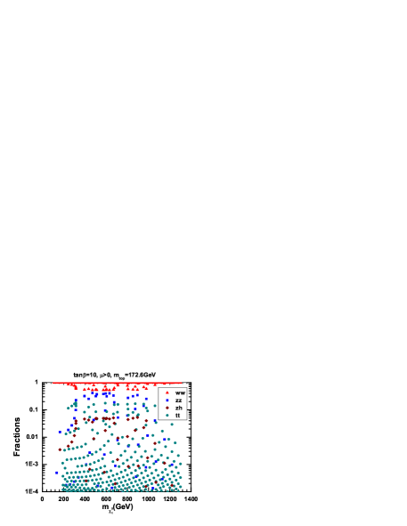
Figure 5: Fractions for neutralinos annihilate into $WW$, $ZZ$, $ZH$ and $t\bar{t}$ as a function of neutralino mass.

The energy distribution of induced neutrino and anti-neutrino from $\widetilde{\chi}_{0}^{1}$ annihilation is the same, thus we can only consider the neutrinos. Because we plan to investigate the neutrino observation by IceCube which has the threshold energy around 50 GeV, we will focus on the flux of high energy neutrino with energy greater than 50 GeV. The production of high energy $\nu_{\mu},\nu_{e}$ neutrinos are the same. The reason is that the produced $\mu$ is stopped by the matter in the Sun before its decay RS88 , thus it mainly produces neutrinos with low energy which we do not consider in this paper. Neutrinos can also be produced from charged pions from hadronization of partons, but they contribute mainly to low energy spectrum. Therefore for high energy neutrinos they are small compared with those from gauge boson and top quark decays. The production of $\nu_{\tau}$ are usually larger than $\nu_{\mu},\nu_{e}$ because $\tau$ lepton decays before it loses energy CFMSSV05 . In summary the neutrino flavor ratios are given by CFMSSV05

$$v_{e}:v_{u}:v_{\tau}:\overline{v}_{e}:\overline{v}_{u}:\overline{v}_{\tau}=1:1:r:1:1:r,$$ (16)

where $r$ varies with the energy of neutrino.

We utilize Calchep comphep ; calchep to generate events, and then use Pythia pythia to handle the decays of intermediate particles contained in the events.

IV.1.1 Annihilation channel $\widetilde{\chi}_{0}^{1}\widetilde{\chi}_{0}^{1}\to W^{+}W^{-},ZZ$

For the annihilation channel $\widetilde{\chi}_{0}^{1}\widetilde{\chi}_{0}^{1}\to W^{+}W^{-},ZZ$, the polarized effects of gauge bosons should be considered, which makes the energy distribution of final state neutrinos different from those without including polarization information BKST07 . In this channel, gauge bosons are transverse polarized with equal up- and down-type polarizations.

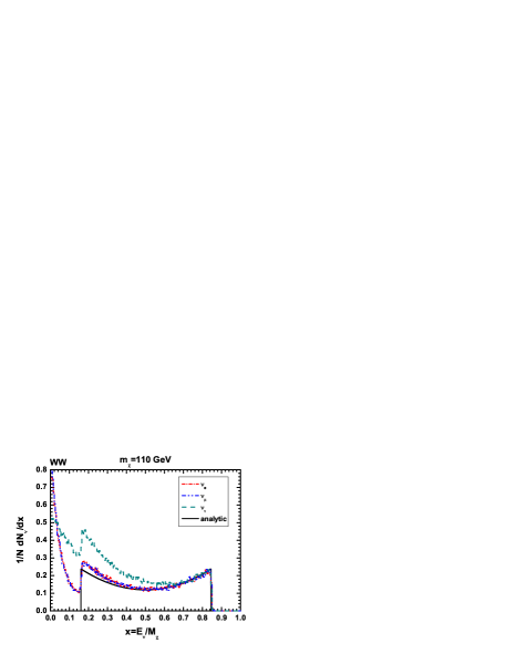
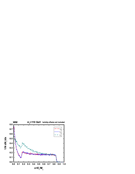
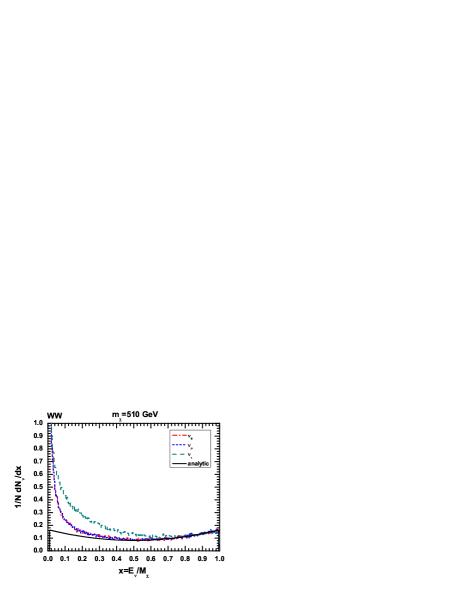
Figure 6: Energy distributions of neutrinos from annihilation channel $\widetilde{\chi}_{0}^{1}\widetilde{\chi}_{0}^{1}\to W^{+}W^{-}$ with neutralino mass 110, 285 and 510 GeV respectively. For the right-top plot, the polarization effect of W gauge bosons are not included. The horizontal axis is energy $x=\frac{{E_{\nu}}}{{m_{\widetilde{\chi}_{0}^{1}}}}$. The vertical axis is $\frac{1}{N}\frac{{dN_{\nu}}}{{dx}}$, where N is the number of annihilation $\widetilde{\chi}_{0}^{1}\widetilde{\chi}_{0}^{1}\to W^{+}W^{-}$ and ${N_{\nu}}$ is the number of neutrinos. The dashed-dot lines, the short dashed lines and the dash lines represent $\nu_{e},\nu_{\mu},\nu_{\tau}$ neutrinos respectively. The solid lines stand for the analytical results of neutrinos which come directly from leptonic decay of polarized W gauge boson produced in $\widetilde{\chi}_{0}^{1}\widetilde{\chi}_{0}^{1}\to W^{+}W^{-}$ BKST07 .

In Fig. 6, the energy distributions of neutrino are shown for several typical neutralino masses. It is obvious that the polarization effects can change the shape of the energy distributions. In the figure the solid lines in the bottom are the analytical results of neutrinos which come directly from W gauge boson leptonic decay BKST07 . The dashed-dot lines in the middle are electron neutrino. We can see that the monte carlo results are higher than analytical results because we include the contributions from varies particle decays. Another distinction between analytical results and monte carlo results is that the latter ones have a higher tail in the low energy region because of W gauge boson hadronic decay and tau lepton decay. The dash lines on the top are the tau neutrinos, which are higher than those of electron neutrinos duo to the contributions from tau lepton decay. The muon neutrino has the same distribution as electron neutrino. Note that in the leptonic decay of W gauge boson, the muon is set to be stable in our simulations, i.e. the neutrino produced by the muon is not counted. The reason is that the $\mu$ loses energy quickly in the Sun and almost at rest before it decays into neutrino RS88 . The decay of tau lepton has significant contributions to tau neutrino compared with analytical result which only include neutrino from W boson CFMSSV05 ; BEO07 . It will enhance the number of muon neutrino via the oscillation effect BEO07 .

In Fig. 7, the energy distributions of neutrinos from annihilation channel $\widetilde{\chi}_{0}^{1}\widetilde{\chi}_{0}^{1}\to ZZ$ are plotted. For 110 GeV neutralino, the ZZ channel has narrower energy distribution compare to that of WW because Z is heavier than W. For heavier neutralino such different energy distribution between Z and W will be smaller. $\frac{1}{N}\frac{{dN_{\nu}}}{{dx}}$ in ZZ channel is higher than that in WW channel because there are two Z bosons and each Z can contribute to both neutrino and anti-neutrino while W boson can not.

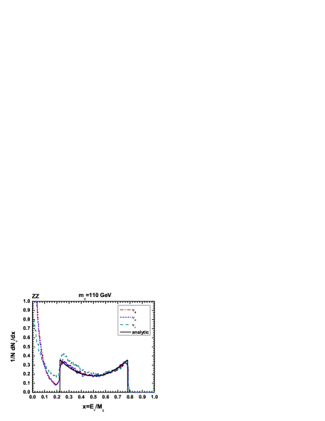
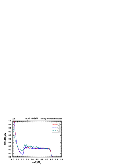
Figure 7: Same as Fig. 6 but for $\widetilde{\chi}_{0}^{1}\widetilde{\chi}_{0}^{1}\to ZZ$.

IV.1.2 Annihilation channel $\widetilde{\chi}_{0}^{1}\widetilde{\chi}_{0}^{1}\to Zh$

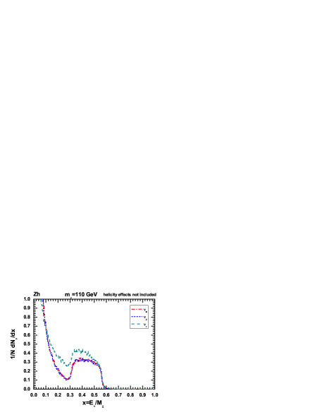
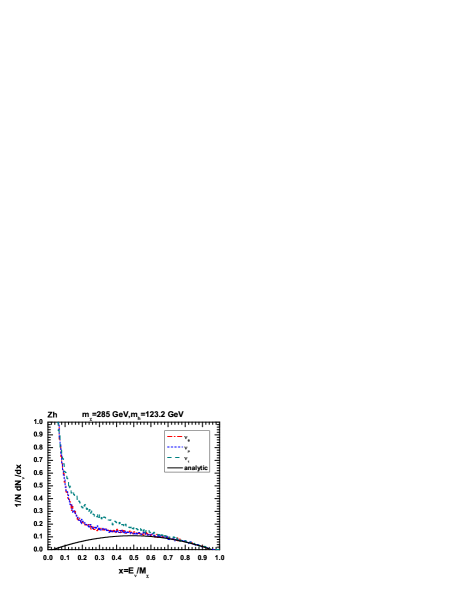
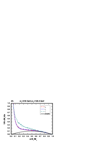
Figure 8: Same as Fig. 6 but for $\widetilde{\chi}_{0}^{1}\widetilde{\chi}_{0}^{1}\to Zh$.

In annihilation channel $\widetilde{\chi}_{0}^{1}\widetilde{\chi}_{0}^{1}\to Zh$, the Z boson is longitudinal polarized BKST07 . The energy distributions of neutrinos are presented in Fig. 8. We also compared the analytic results with our full simulations which include both polarization effects and various particle decays. Once again, the full simulations have higher tau neutrino production, right energy distributions shape after including polarization effects, as well as the higher low energy tail from lepton decay and quark hadronic decays.

IV.1.3 Annihilation channel $\widetilde{\chi}_{0}^{1}\widetilde{\chi}_{0}^{1}\to t\overline{t}$

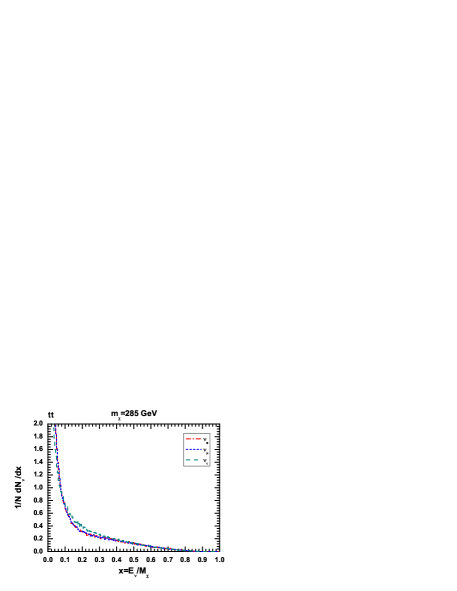
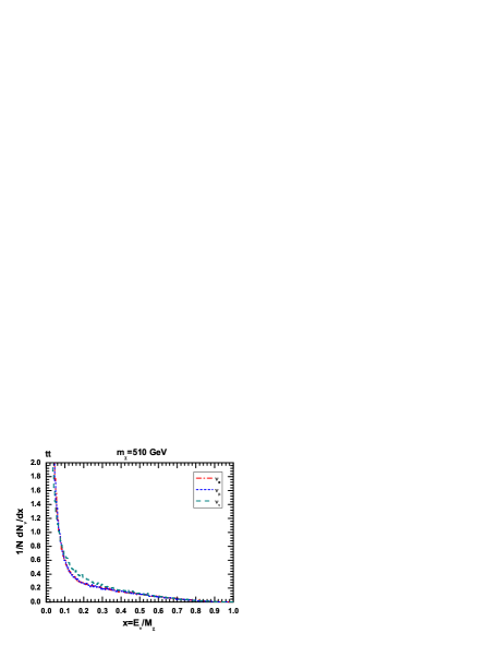
Figure 9: Energy distributions of neutrinos from annihilation channel $\widetilde{\chi}_{0}^{1}\widetilde{\chi}_{0}^{1}\to t\overline{t}$ with neutralino mass 285 and 510GeV respectively. The conventions are the same as those in Fig. 6 .

For annihilation channel $\widetilde{\chi}_{0}^{1}\widetilde{\chi}_{0}^{1}\to t\overline{t}$, it has small contributions to our final results. For simplicity we utilize WimpSim to generate the signals with averaged t-quark polarizations wimpsim . The energy distributions are shown in Fig. 9.

IV.2 The propagation of neutrino

The neutrinos produced at the solar center will interact with the nucleus in the Sun during their propagation to the solar surface. The matter effects include the neutral current(NC) effects, the charged current(CC) effects and tau neutrino $\nu_{\tau}$ re-injection from secondary tau lepton decay. From solar center to the Earth the oscillation effects of neutrinos are also important and must be taken into account. In the density matrix method, the evolution equation is CFMSSV05

$$\frac{{d\rho}}{{dr}}=-i[H,\rho]+\left.{\frac{{d\rho}}{{dr}}}\right|_{NC}+\left.{\frac{{d\rho}}{{dr}}}\right|_{CC}+\left.{\frac{{d\rho}}{{dr}}}\right|_{0}.$$ (17)

Here the first term at the RHS describes the vacuum oscillation. The second and third terms describe NC and CC effect separately, including neutrino absorption, scattering and $\nu_{\tau}$ re-injection. The last term $\left.{\frac{{d\rho}}{{dr}}}\right|_{0}=\delta(r)\delta_{ij}\frac{1}{N}\frac{dN}{dE_{\nu}}$ is the initial neutrino at the production point.

We use Monte Carlo program WimpSim which is event-based code to handle the propagation process of neutrinos from the Sun center to a distance of 1 astronomical unit (AU) wimpsim . WimpSim treats three flavor neutrino interactions and oscillations in one framework. The equivalence between the Monte Carlo method and the density matrix formalism used in CFMSSV05 has been discussed in Ref. BEO07 . The detail Monte Carlo simulations allow us tracing every neutrino event and determining final $\mu$ signals with the concrete energy and angle information. Thus this approach can provide more realistic events. We take the neutrino oscillation parameters which given by global fit to neutrino experiments MSTV07 ( The 2007 updated values in Ref. MSTV07 have been used ). Explicitly, we choose $\theta_{{\rm{12}}}=34.4^{\circ}$, $\theta_{{\rm{13}}}=0^{\circ}$ and $\theta_{{\rm{23}}}=45^{\circ}$, the mass-squared difference $\Delta m_{21}^{2}=7.6\times 10^{-5}eV^{2}$, $\Delta m_{31}^{2}=2.4\times 10^{-3}eV^{2}$ and CP-violating phase $\delta=0$.

V The detection of neutrino by IceCube

When the Sun is below the horizon, the up-going muon-neutrinos may produce high energy muons in the Earth. When these muons travel in the ice, they will lose their energy via scattering with other matter. The IceCube in south pole is designed to detect such kind of muons.

The analytical formula of final muon flux at the detector has been given in Ref. BKST07 . The muon energy loss is given as DRSS00

$$\frac{dE}{dx}=-\alpha-\beta E,$$ (18)

where $\alpha$ and $\beta$ are empirical parameters. The distance that a muon travels in the Earth before its energy drops below threshold energy $E^{thr}$, is called muon range which is given as

$$R_{\mu}(E)=\frac{1}{\rho\beta}\ln(\frac{\alpha+\beta E}{\alpha+\beta E^{thr}}).$$ (19)

Instead of utilizing above analytical formulas to calculate muon flux, we use WimpSim to get muon flux based on event-by-event Monte Carlo simulation. After obtaining the neutrino events at the surface of the Earth as discussed in the previous section, we then simulate the neutrinos propagation in the Earth and the final flux of muons. The muons are induced from CC interaction at actual neutrino telescope IceCube, which is mainly characterized by $E^{thr}$, $R_{\mu}(E)$, $A_{eff}$ and its geographical position. We calculate the effective detecting area $A_{eff}$ as that in Ref. GHM05 . Note that $A_{eff}$ in Eqn. 1 is also function of final muon energy. The WimpEvent uses a simple model to treat the Earth orbit and obtain the detector time-dependent location for each neutrino event BEO07 .

Comparing with analytical formula, the simulation can give more information about muon flux. The muon energy at the detector can be given by this simulation, while analytical formula only gives muon energy at the vertex where neutrinos convert into muons. The information about angle between muon velocity and the direction from the Sun to the detector can also be obtained which is important to reduce background.

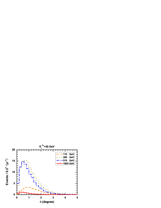
Figure 10: The muon events ($\mu^{+}+\mu^{-}$) distributions in IceCube as a function of angle $\theta$ which is defined as angle between the muon velocity and the direction from Sun to the detector. The IceCube $1^{0}$ angle resolution is not reflected here, and every bin is taken as $0.2^{0}$. The threshold energy for muon is taken as $50GeV$.

We show our final results for some benchmark points in Fig. 10 after multiplying initial dark matter annihilation rate in the core of the Sun. Here we have summed the $\mu^{\pm}$ events together and taken $E^{thr}=50GeV$ into account. After produced from charged current scattering process, the muon may have multiple Coulomb scattering in the ice E93 ; EG95 . Thus the final direction of muon velocity is not the exactly same direction from the Sun to the detector. From Fig. 10, we can see the deviation of muon direction is not large, and most of muon events are in the scope of $\pm 2^{0}$ around the direction from the Sun to the detector. And the signals from high energy neutrinos produced by heavy massive neutralinos annihilation are less affected by Coulomb scattering as naive expectation. Note that the IceCube can reach angle resolution as small as $1^{0}$ Aetal04 , our results suggest a possible method to reduce the background events from other sources.

Now we switch to the discussions on the backgrounds. The largest backgrounds come from comic ray. When cosmic ray interacts in the atmosphere around the Earth, high energy neutrinos would be created and travel to the detector. During the propagation, the neutrinos can produce muons atmnu ; E93 ; HKKMS07 . Such kind of high energy neutrinos do not have special direction. Therefore if we only observe the events around the special direction from Sun to the detector, the backgrounds would be dramatically reduced. Other possible background are muons from cosmic ray interacting with the atmosphere around the Earth atmmu and neutrinos from cosmic ray interacting with particles in the Sun’s corona suncorona . However these two kinds of backgrounds are not important in the detection of muons at IceCube. For the rough estimate, we only take the atmosphere neutrino backgrounds into account. The atmosphere neutrino flux are taken from Ref. HKKMS07 and method to estimate the muon rate from Ref. BKST07 . The resulting background muons are not the function of $E^{fin}$ but for $E^{0}$, i.e. energy of the induced muon. It should be noted that more accurate results need Monte Carlo simulation.

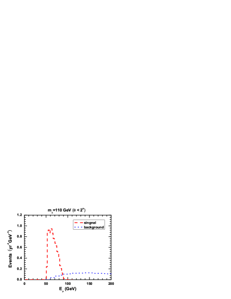
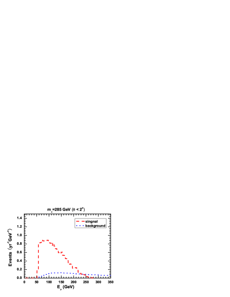
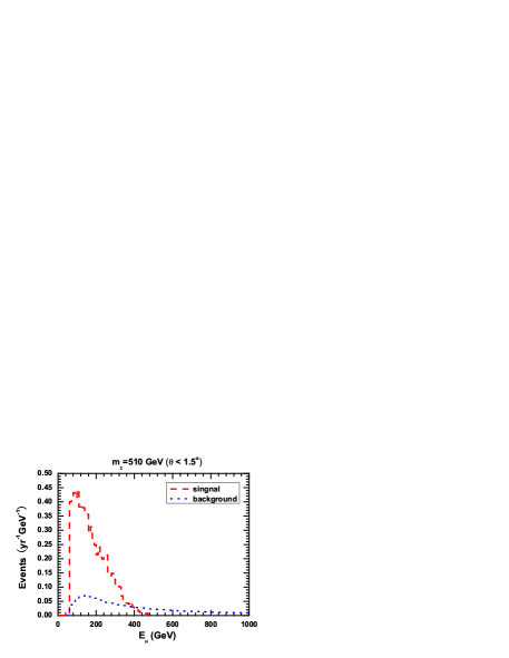
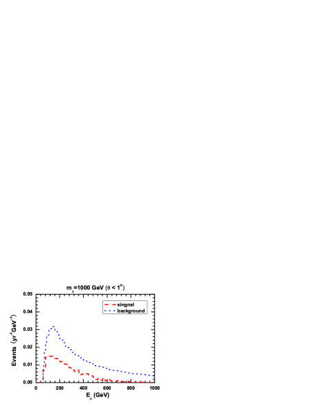
Figure 11: Differential muon rate in IceCube as a function of energy of muon for several neutralino mass as 110, 285, 510 and 1000 GeV. We applied different angular cuts on muon zenith angle in order to get better significance according to the result of Fig. 10. The red dashed (the blue dotted ) lines represent the muon signals (the atmosphere backgrounds).

Point	$m_{\chi}$(GeV)	$m_{0}$(TeV)	$m_{3/2}$(TeV)	$\mu$(GeV)	$R_{h}$	$\sigma_{SD}(pb)$	$C_{\odot}(yr^{-1})$
A	$110$	2.9	34	420	4.4 $\%$	5.1$\times 10^{-5}$	8.3$\times 10^{29}$
B	$285$	6.1	88	498	7.1 $\%$	4.2$\times 10^{-5}$	1.0$\times 10^{29}$
C	$510$	9.5	162	620	19.2 $\%$	5.0$\times 10^{-5}$	4.1$\times 10^{28}$
D	$1000$	15.3	314	1120	14.5 $\%$	1.1$\times 10^{-5}$	2.2$\times 10^{27}$

Table 1: Several benchmark points (point A-D) in mAMSB model. $R_{h}$ is the higgsino fraction $\left|{N_{13}}\right|^{2}+\left|{N_{14}}\right|^{2}$, $\sigma_{SD}$ is the spin-dependent cross section and $C_{\odot}$ is the neutralino capture rate for the Sun.

Point	$\frac{{\sigma_{WW}}}{{\sigma_{tot}}}$	$\frac{{\sigma_{ZZ}}}{{\sigma_{tot}}}$	$\frac{{\sigma_{t\overline{t}}}}{{\sigma_{tot}}}$	$\frac{{\sigma_{Zh}}}{{\sigma_{tot}}}$	$\theta cut$ (∘)	$Sig$	$BG$	$\sigma_{stat}$
A	100.0$\%$	0.0$\%$	0.0$\%$	0.0$\%$	2.0	23.3	24.1	4.7
B	99.1$\%$	0.0$\%$	0.9$\%$	0.0$\%$	2.0	102.1	24.1	20.8
C	95.6$\%$	0.2$\%$	4.2$\%$	0.0$\%$	1.5	70.3	13.6	19.1
D	96.9$\%$	0.1$\%$	3.0$\%$	0.0$\%$	1.0	3.0	6.0	1.2

Table 2: One year total muon rate at IceCube for various benchmark points (point A-D) where muons satisfy $E_{thr}<E_{\mu}<300GeV$ with $E_{thr}=50GeV$. Here $\frac{{\sigma_{WW}}}{{\sigma_{tot}}},\frac{{\sigma_{ZZ}}}{{\sigma_{tot}}},\frac{{\sigma_{t\overline{t}}}}{{\sigma_{tot}}},\frac{{\sigma_{Zh}}}{{\sigma_{tot}}}$ are the fractions of annihilation channels $WW,ZZ,Zh,t\overline{t}$ separately. $\theta_{CUT}$ is the angular cut for zenith angle of muon. Sig is the annual muon rate and BG is the annual muon background from atmosphere neutrino. We define statistical significance as $\sigma_{stat}=S/\sqrt{B}$.

Our final results are depicted in Fig. 11, Tab. 1 and 2. The four parameter points are almost dominant by annihilation channel WW which is one of the characters of AMSB model. All four benchmark points, which satisfy all the constraints from other experiments, have the same order of magnitude of $\sigma_{SD}$, which is essential for the muon detection at IceCube. Point A with 110GeV neutralino has much smaller signal than that of Point B with $285GeV$ neutralino because the former is affected by the energy threshold and muon range $R_{\mu}$. Point C and D with heavier neutralino are less affected by the energy threshold but the capture rate $C_{\odot}$ is suppressed. We applied different angular cut on zenith angle of muon to get better statistical significance according to the results in Fig. 10. From Tab. 2, we can see the signal annual events can reach 102 for Point B and the statistical significance $\sigma_{stat}$ can reach more than 20. Based on our numerical estimation, we can obtain the rule of thumb for IceCube to discover high energy neutrino from Sun in AMSB model, i.e. $\sigma_{SD}>10^{-5}pb$. It should be noted that $N_{13}^{2}+N_{14}^{2}>4\%$ approximately corresponds to the condition $\sigma_{SD}>10^{-5}pb$ based on the results in Fig. 1 and 3.

VI Conclusions and discussions

In this paper in the mAMSB model we have investigated the muon event rate at IceCube. Such kind of muon events are induced by high energy neutrino flux from neutralino annihilation in the Sun. We studied the detail energy and angular spectrum of the final muons at the detector based on event-by-event simulation by using Monte Carlo code WimpSim. More precisely we simulated the processes since the production of neutrino via neutralino annihilation in the core of the Sun, neutrino propagation from the Sun to the Earth, as well as the converting processes from neutrino to muon. Our results show that in the mAMSB model it is possible to observe the energetic muons at IceCube, provided that the lightest neutralio has relatively large higgsino component, as a rule of thumb $N_{13}^{2}+N_{14}^{2}>4\%$ or equivalently $\sigma_{SD}>10^{-5}pb$. Especially for our benchmark Point B (see Tab. 1), the signal annual events can reach 102 and the statistical significance can reach more than 20. This parameter space is very similar to the ’focus point’ region in mSUGRA model.

It should be emphasized that our study has much more improvement compared to previous investigations. For example, we include both polarized effect of gauge bosons and secondary neutrinos from the decay of leptons and quarks. The polarization effects of the gauge bosons can have important influences on the neutrino energy spectrum, as shown in our results and in Ref. BKST07 . The secondary neutrinos are usually handled by Pythia, for example in Ref. CFMSSV05 and WimpSim wimpsim . But none of them include both effects. We use Monte Carlo code WimpSim to handle the interactions includes NC effect, CC effect and tau neutrino $\nu_{\tau}$ re-injection from secondary tau lepton decay. Comparing with the previous analytical result, the Monte Carlo approach can not only give the same evolution results as those by solving Eqn. 17 but also the angular distribution of muons as shown in Fig. 10. With the angular distributions at hand, we can choose $2^{\circ}$ as normal cut in range $100GeV<m_{\widetilde{\chi}_{0}^{1}}<500GeV$ to reduce the background from atmosphere neutrinos. With heavier neutralinos, smaller cut can be chosen to further reduce the background. As shown in Ref. H08 , the light neutralino in this scenario is disfavored. Thus the techniques to suppress background in order to extract low signal events for heavy neutralino is very important.

Last but not least, we want to emphasize that the final energy spectra of muons will have similar shape as those in Fig. 11 in the mAMSB model, because the annihilation of neutralinos are almost $\widetilde{\chi}_{0}^{1}\widetilde{\chi}_{0}^{1}\to W^{+}W^{-}$. Thus it is possible to distinguish among AMSB model from other SUSY breaking scenarios due to different annihilation modes if enough muons can be collected.

VII Acknowledgements

This work was supported in part by the Natural Sciences Foundation of China (No. 10775001 and 10635030), and the trans-century fund of Chinese Ministry of Education.

References

- (1) D. N. Spergel et al. [WMAP Collaboration], Astrophys. J. Suppl. 170, 377 (2007).
- (2) For reviews, see G. Jungman, M. Kamionkowski and K. Griest, Phys. Rept 267, 195 (1996); G. Bertone, D. Hooper and J. Silk, Phys. Rept 405, 279 (2005).
- (3) D. O. Caldwell, R. M. Eisberg, D. M. Grumm, M. S. Witherell, B. Sadoulet, F. S. Goulding and A. R. Smith, Phys. Rev. Lett. 61, 510 (1988); D. O. Caldwell et al., Phys. Rev. Lett. 65, 1305 (1990); D. Reusser et al., Phys. Lett. B 255, 143 (1991).
- (4) J. L. Feng, A. Rajaraman and F. Takayama, Phys. Rev. Lett 91, 011302 (2003).
- (5) H. Goldberg, Phys. Rev. Lett 50, 1419 (1983); J. R. Ellis, J. S. Hagelin, D. V. Nanopoulos, K. A. Olive and M. Srednicki, Nucl. Phys. B 238, 453 (1984).
- (6) K. L. Chan, U. Chattopadhyay and P. Nath, Phys. Rev. D 58, 096004 (1998).
- (7) J. L. Feng, K. T. Matchev and T. Moroi, Phys. Rev. Lett 84, 2322 (2000) and Phys. Rev. D 61, 075005 (2000).
- (8) J. L. Feng and F. Wilczek, Phys. Lett. B 631, 170 (2005).
- (9) H. Baer, T. krupovnickas, S. Profumo and P. Ullio, JHEP 0510, 020 (2005).
- (10) J. L. Feng, K. T. Matchev and F. Wilczek, Phys. Lett. B 482, 388 (2000) and Phys. Rev. D 63, 045024 (2001).
- (11) L. Randall and R. Sundrum, Nucl. Phys. B 557, 79 (1999).
- (12) G. F. Giudice, M. A. Luty, H. Murayama and R. Rattazzi, JHEP 9812, 027 (1998).
- (13) T. Gherghetta, G. F. Giudice and J. D. Wells, Nucl. Phys. B 559, 27 (1999).
- (14) T. Moroi and L. Randall, Nucl. Phys. B 570, 455 (2000).
- (15) U. Chattopadhyay, D. Das, P. Konar and D. P. Roy, Phys. Rev. D 75, 073014 (2007).
- (16) J. D. Wells, Phys. Rev. D 71, 015013 (2005).
- (17) J. Hisano, S. Matsumoto, M. Nagai, O. Saito, M. Senami, Phys. Lett. B 646, 34 (2007).
- (18) I. F. M. Albuquerque, L. Hui and E. W. Kolb, Phys. Rev. D 64, 083504 (2001); P. Crotty, Phys. Rev. D 66, 063504 (2002).
- (19) K. M. Belotsky, M. Y. Khlopov and K. I. Shibaev, Part. Nucl. Lett. 108, 5 (2001); K. M. Belotsky, T. Damour and M. Y. Khlopov, Phys. Lett. B 529, 10 (2002).
- (20) V. D. Barger, F. Halzen, D. Hooper and C. Kao, Phys. Rev. D 65, 075022 (2002).
- (21) D. Hooper and G. D. Kribs, Phys. Rev. D 67, 055003 (2003).
- (22) D. Hooper and G. Servant, Astropart. Phys 24, 231 (2005).
- (23) D. Hooper, H. Nunokawa, O. L. G. Peres and R. Zakanovich Funchal, Phys. Rev. D 67, 013001 (2003); F. Halzen and D. Hooper, JCAP 0401, 002 (2004) and Phys. Rev. D 73, 123507 (2006).
- (24) J. Lundberg and J. Edsjo, Phys. Rev. D 69, 123505 (2004).
- (25) M. Cirelli, N. Fornengo, T. Montaruli, I. Sokalski, A. Strumia and F. Vissani, Nucl. Phys. B 727, 99 (2005).
- (26) V. Barger, W. Y. Keung, G. Shaughnessy and A. Tregre, Phys. Rev. D 76, 095008 (2007).
- (27) R. Lehnert and T. J. Weiler, arXiv:/0708.1035 [hep-ph].
- (28) W. H. Press and D. N. Spergel, Astrophys. J 296, 679 (1985).
- (29) J. Silk, K. Olive and M. Srednicki, Phys. Rev. Lett 55, 257 (1985); L. M. Krauss, M. Srednicki and F. Wilczek, Phys. Rev. D 33, 2079 (1986); T. K. Gaisser, G. Steigman and S. Tilav, Phys. Rev. D 34, 2206 (1986).
- (30) J. S. Hagelin, K. W. Ng and K. A. Olive, Phys. Lett. B 180, 375 (1986).
- (31) J. Ahrens et al., IceCube Preliminary Design Document, (2001).
- (32) J. Ahrens et al. [IceCube Collaboration], Astropart. Phys. 20, 507 (2004).
- (33) S. Desai et al. [Super-Kamiokande Collaboration], Phys. Rev. D 70, 083523 (2004).
- (34) E. Andres et al., Astropart. Phys. 13, 1 (2000).
- (35) E. Aslanides et al. [ANTARES Collaboration], arXiv:astro-ph/9907432.
- (36) J. Edsjo, TSL/ISV-93-0091 preprint, Uppsala University, ISSN 0284-2769.
- (37) A. Pukhov et al., arXiv:hep-ph/9908288.
- (38) A. Pukhov, arXiv:hep-ph/0412191.
- (39) J. Edsjo, WimpSim Neutrino Monte Carlo, http://www.physto.se/~edsjo/wimpsim/
- (40) M. Blennow, J. Edsjo and T. Ohlsson, JCAP 0801, 021 (2008).
- (41) T. Sjostrand, S. Mrenna and P. Skands, JHEP 0605, 026 (2006).
- (42) P. Gondolo, J. Edsjo, P. Ullio, L. Bergstom, M. Schelke and E.A. Baltz, JCAP 0407 (2004) 008.
- (43) J. Edsjo, Nusigma 1.15.
- (44) L. Bergstrom, J. Edsjo and P. Gondolo, Phys. Rev. D 55, 1765 (1997) and Phys. Rev. D 58, 103519 (1998).
- (45) J. Edsjo, arXiv:hep-ph/9704384.
- (46) M. C. Gonzalez-Garcia, F. Halzen and M. Maltoni, Phys. Rev. D 71, 093010 (2005).
- (47) A. Pomarol and R. Rattazzi, JHEP 9905, 013 (1999).
- (48) D. E. Kaplan and G. D. Kribs, JHEP 0009, 048 (2000).
- (49) Z. Chacko and M. A. Luty, JHEP 0205, 047 (2002).
- (50) R. N. Mohapatra, N. Setzer and S. Spinner, Phys. Rev. D 77, 053013 (2008) and arXiv:0802.1208 [hep-ph].
- (51) J. L. Feng and T. Moroi, Phys. Rev. D 61, 095004 (2000).
- (52) A. Djouadi, J. L. Kneur and G. Moultaka, Comput. Phys. Commun. 176, 426 (2007).
- (53) G. F. Giudice and A. Romanino, Nucl. Phys. B 699, 65 (2004).
- (54) G. Belanger, F. Boudjema, A. Pukhov and A. Semenov, Comput. Phys. Commun 176, 367 (2007).
- (55) J. Hisano, S. Matsumoto, M. M. Nojiri, O. Saito, Phys. Rev. D 71, 063528 (2005).
- (56) J. Hisano, S. Matsumoto, O. Saito and M. Senami, Phys. Rev. D 73, 055004 (2006).
- (57) E. A. Baltz and J. Edsjo, Phys. Rev. D 59, 023511 (1998); D. Hooper and J. Silk, Phys. Rev. D 71, 083503 (2005); S. Profumo and P.Ullio, JCAP 0407, 006 (2004).
- (58) D. Hooper and B. L. Dingus, Phys. Rev. D 70, 113007 (2004); arxiv:astro-ph/0212509.
- (59) H. Yuksel, S. Horiuchi, J. F. Beacom and S. Ando, Phys. Rev. D 76, 123506 (2007).
- (60) D. Hooper, arXiv:/0801.4378 [hep-ph].
- (61) K. Jedamzik, Phys. Rev. D 70, 083510 (2004).
- (62) For example to see, J. L. Feng, T. Moroi, L. Randall, M. Strassler and S. Su, Phys. Rev. Lett 83, 1731 (1999); H. Baer, J. K. Mizukoshi and X. Tata Phys. Lett. B 488, 367 (2000); D. K. Ghosh, P. Roy and S. Roy JHEP 0008, 031 (2000); D. K. Ghosh, A. Kundu, P. Roy and S. Roy, Phys. Rev. D 64, 115001 (2001); A. Datta, P. Konar and B. Mukhopadhyaya, Phys. Rev. Lett 88, 181802 (2002); A. J. Barr, C. G. Lester, M. A. Parker, B. C. Allanach and P. Richardson, JHEP 0303, 045 (2003); A. Datta, K. Huitu, Phys. Rev. D 67, 115006 (2003); T. Honkavaara, K. Huitu, S. Roy, Phys. Rev. D 73, 055011 (2006).
- (63) P. Ullio, JHEP 0106, 053 (2001).
- (64) D. Hooper, L. T. Wang. Phys. Rev. D 69, 035001 (2004).
- (65) J. Hisano, S. Matsumoto, M. M. Nojiri, O. Saito, Phys. Rev. D 71, 015007 (2005).
- (66) T. T. E. Group et al. [CDF Collaboration], arXiv:0803.1683 [hep-ex].
- (67) R. Barate et al. [LEP Working Group for Higgs boson searches], Phys. Lett. B 565, 61 (2003).
- (68) E. Barberio et al. [Heavy Flavor Averaging Group (HFAG) Collaboration], arXiv:0704.3575 [hep-ex].
- (69) G. W. Bennett et al. [Muon G-2 Collaboration], Phys. Rev. D 73, 072003 (2006).
- (70) K. Hagiwara, A. D. Martin, D. Nomura, T. Teubner Phys. Lett. B 649, 173 (2007).
- (71) A. Gould, Astrophys. J. 321, 338 (1992).
- (72) W. M. Yao et al. [Particle Data Group], J. Phys. G 33 (2006) 1.
- (73) J. Angle et al. [XENON Collaboration], Phys. Rev. Lett. 100, 021303 (2008).
- (74) M. Kamionkowski, Phys. Rev. D 44, 3021 (1991).
- (75) M. T. Ressell, M. B. Aufderheide, S. D. Bloom, K. Griest, G. J. Mathews and D. A. Resler, Phys. Rev. D 48, 5519 (1993).
- (76) H. Baer and M. Brhlik, Phys. Rev. D 57, 567 (1998).
- (77) J. Ellis and M. Karliner, Phys. Lett. B 313, 131 (1993).
- (78) S. Ritz and D. Seckel, Nucl. Phys. B 304 877 (1988).
- (79) M. Maltoni, T. Schwetz, M. A. Tortola and J. W. F. Valle, New J. Phys. 6, 122 (2004), arXiv:hep-ph/0405172v6.
- (80) S. Iyer Dutta, M. H. Reno, I. Sarcevic and D. Seckel, Phys. Rev. D 63, 094020 (2001).
- (81) J. Edsjo and P. Gondolo, Phys. Lett. B 357, 595 (1995).
- (82) M. Honda, T. Kajita, K. Kasahara, S. Midorikawa and T. Sanuki, Phys. Rev. D 75, 043006 (2007).
- (83) L. V. Volkova, Yad. Fiz. 31, 1510 (1980) [Sov. J. Nucl. Phys. 31, 784 (1980)]; T. K. Gaisser and T. Stanev, Phys. Rev. D 30, 985 (1984); T. K. Gaisser, T. Stanev and G. Barr, Phys. Rev. D 38, 85 (1988).
- (84) P. Lipari, Astropart. Part 1, 195 (1993).
- (85) D. Seckel, T. Stanev and T. K. Gaisser, Astrophys. J 382, 652 (1991); G. Ingelman and M. Thunman, Phys. Rev. D 54, 4385 (1996); G. L. Fogli, E. Lisi, A. Mirizzi, D. Montanino and P. D. Serpico, Phys. Rev. D 74, 093004 (2006).