Intertwining symmetry algebras of quantum superintegrable systems on the hyperboloid

Abstract

A class of quantum superintegrable Hamiltonians defined on a two-dimensional hyperboloid is considered together with a set of intertwining operators connecting them. It is shown that such intertwining operators close a $su(2,1)$ Lie algebra and determine the Hamiltonians through the Casimir operators. By means of discrete symmetries a broader set of operators is obtained closing a $so(4,2)$ algebra. The physical states corresponding to the discrete spectrum of bound states as well as the degeneration are characterized in terms of unitary representations of $su(2,1)$ and $so(4,2)$.

1 Introduction

In this work we will consider a quantum superintegrable system living in a two-dimensional hyperboloid of two-sheets. Although this system is well known in the literature [1]-[6] and can be dealt with standard procedures [7]-[9], it will be studied here under a different point of view based on the properties of intertwining operators (IO), a form of Darboux transformations [10]. We will see how this approach can give a simple explanation of the main features of this physical system. The intertwining operators and integrable Hamiltonians have been studied in previous references [11]-[14], but we will supply here a thorough non-trivial application by means of this example. Besides, there are several points of interest for the specific case here considered because of the non-compact character.

The intertwining operators are first order differential operators connecting different Hamiltonians in the same class (called hierarchy) and they are associated to separable coordinates of the Hamiltonians. We will obtain just a complete set of such intertwining operators, in the sense that any of the Hamiltonians of the hierarchy can be expressed in terms of these operators.

In our case the initial IO’s close an algebraic structure which is the non-compact Lie algebra $su(2,1)$ (see [15] for a compact case). In a second step we will get a larger $so(4,2)$ Lie algebra of operators. This structure allows us to characterize the discrete spectrum and the corresponding eigenfunctions of the system by means of (infinite dimensional) irreducible unitary representations (iur). The construction of such representations, as it is known, is not so standard as for compact Lie algebras. We will compute the ground state and characterize the representation space of the wave-functions which share the same energy. Notice that these systems include also a continuum spectrum, but we will not go into this point here.

The organization of the paper is as follows. Section 2 introduces the superintegrable Hamiltonians and Section 3 shows how to build the IO’s connecting hierarchies of these kind of Hamiltonians. In Section 4 it is seen that these operators close a $su(2,1)$ algebra. The Hamiltonians are related to the Casimirs of such an algebra, while the discrete spectrum of the Hamiltonians is related to unitary representations (iur’s) of $su(2,1)$. Next, in Section 5 a broader class of IO’s is defined leading to the $so(4,2)$ Lie algebra, and it is shown how this new structure helps to understand better the Hamiltonians in the new hierarchies. Finally, some remarks and conclusions in Section 6 will end the paper.

2 Parametrizations of the two-sheet hyperboloid

Let us consider the two-dimensional two-sheet hyperboloid $s_{0}^{2}+s_{1}^{2}-s_{2}^{2}=-1$, where we define the following Hamiltonian

$$H_{\ell}=J_{2}^{2}-J_{1}^{2}-J_{0}^{2}-\frac{l_{2}^{2}-\frac{1}{4}}{s_{2}^{2}}+\frac{l_{1}^{2}-\frac{1}{4}}{s_{1}^{2}}+\frac{l_{0}^{2}-\frac{1}{4}}{s_{0}^{2}},$$ (2.1)

where $\ell=(l_{0},\,l_{1},\,l_{2})\in\mathbb{R}^{3}$, and the differential operators

$$J_{0}=s_{1}\partial_{2}+s_{2}\partial_{1},\quad J_{1}=s_{2}\partial_{0}+s_{0}\partial_{2},\quad J_{2}=s_{0}\partial_{1}-s_{1}\partial_{0},$$ (2.2)

constitute a realization of the $so(2,1)$ Lie algebra with Lie commutators

$$[J_{0},J_{1}]=-J_{2},\qquad[J_{2},J_{0}]=J_{1},\qquad[J_{1},J_{2}]=J_{0}.$$

The generator $J_{2}$ corresponds to a rotation around the axis $s_{2}$, while the generators $J_{0}$ and $J_{1}$ give pseudo-rotations (i.e., non-compact rotations) around the axes $s_{0}$ and $s_{1}$, respectively. The Casimir operator

$$C=J_{0}^{2}+J_{1}^{2}-J_{2}^{2}$$

gives the ‘kinetic’ part of the Hamiltonian.

We can parametrize the hyperbolic surface by means of the ‘analogue’ of the spherical coordinates

$$s_{0}={\sinh\xi}\,\cos{\theta},\quad s_{1}={\sinh\xi}\,\sin{\theta},\quad s_{2}={\cosh{\xi}},$$ (2.3)

where $0\leq\theta<2\pi$ and $0\leq\xi<\infty$. In these coordinates, the infinitesimal generators (2.2) take the following expressions

$$J_{0}=\sin{\theta}\,\partial_{\xi}+\cos{\theta}\,{\coth\xi}\,\partial_{\theta},\quad J_{1}=\cos{\theta}\,\partial_{\xi}-\sin{\theta}\,{\coth\xi}\,\partial_{\theta},\quad J_{2}=\partial_{\theta}\,.$$ (2.4)

It is easy to check that the generators $J_{i}$, $i=1,2,3$, are anti-Hermitian inside the space of square-integrable functions with the invariant measure $d\mu(\theta,\xi)=\sinh\xi\,d\theta d\xi$. Using the coordinates (2.3), the Hamiltonian (2.1) has the expression

$$H_{\ell}=-\partial_{\xi}^{2}-{\coth\xi}\,\partial_{\xi}-\frac{l_{2}^{2}-\frac{1}{4}}{\cosh^{2}\xi}+\frac{1}{\sinh^{2}\xi}\left[-\partial_{\theta}^{2}+\frac{l_{1}^{2}-\frac{1}{4}}{\sin^{2}\theta}+\frac{l_{0}^{2}-\frac{1}{4}}{\cos^{2}\theta}\right].$$ (2.5)

Therefore, $H_{\ell}$ can be separated in the variables $\xi$ and $\theta$. Choosing its eigenfunctions $\Phi_{\ell}$, $H_{\ell}\Phi_{\ell}=E\Phi_{\ell}$, in the form

$$\Phi_{\ell}(\theta,\xi)=f(\theta)\,g(\xi),$$ (2.6)

we get the separated equations

$$H_{l_{0},l_{1}}^{\theta}f(\theta)\equiv\left[-\partial_{\theta}^{2}+\frac{l_{1}^{2}-\frac{1}{4}}{\sin^{2}\theta}+\frac{l_{0}^{2}-\frac{1}{4}}{\cos^{2}\theta}\right]f(\theta)=\alpha\,f(\theta)$$ (2.7)

and

$$\left[-\partial_{\xi}^{2}-{\coth\xi}\,\partial_{\xi}-\frac{l_{2}^{2}-\frac{1}{4}}{\cosh^{2}\xi}+\frac{\alpha}{\sinh^{2}\xi}\right]g(\xi)=E\,g(\xi),$$ (2.8)

where $\alpha>0$ is a separation constant.

3 A complete set of intertwining operators

The second order operator at the l.h.s. of (2.7) in the variable $\theta$ can be factorized in terms of first order operators [16, 17]

$$H_{l_{0},l_{1}}^{\theta}=A^{+}_{l_{0},l_{1}}A^{-}_{l_{0},l_{1}}+\lambda_{l_{0},l_{1}},$$

being

$$A_{l_{0},l_{1}}^{\pm}=\pm\partial_{\theta}-(l_{0}+1/2)\,{\tan{\theta}}+(l_{1}+1/2)\,{\cot{\theta}},\quad\lambda_{l_{0},l_{1}}=(1+l_{0}+l_{1})^{2}.$$ (3.1)

The Hamiltonian can also be rewritten in terms of the triplet ($A^{\pm}_{l_{0}-1,l_{1}-1},\lambda_{l_{0}-1,l_{1-1}}$)

$$H_{l_{0},l_{1}}^{\theta}=A_{l_{0}-1,l_{1}-1}^{-}A_{l_{0}-1,l_{1}-1}^{+}+\lambda_{l_{0}-1,l_{1}-1}=A_{l_{0},l_{1}}^{+}A_{l_{0},l_{1}}^{-}+\lambda_{l_{0},l_{1}}.$$ (3.2)

In this way we get a hierarchy of Hamiltonians

$$\cdots,H_{{l_{0}-1},{l_{1}-1}}^{\theta},H_{{l_{0}},{l_{1}}}^{\theta},H_{{l_{0}+1},{l_{1}+1}}^{\theta},\cdots,H_{{l_{0}+n},{l_{1}+n}}^{\theta},\cdots$$ (3.3)

satisfying the following recurrence relations

$$\begin{array}[]{l}A_{l_{0}-1,l_{1}-1}^{-}H_{l_{0}-1,l_{1}-1}^{\theta}=H_{l_{0},l_{1}}^{\theta}A_{l_{0}-1,l_{1}-1}^{-},\\[6.45831pt] A_{l_{0}-1,l_{1}-1}^{+}H_{l_{0},l_{1}}^{\theta}=H_{l_{0}-1,l_{1}-1}^{\theta}A_{l_{0}-1,l_{1}-1}^{+}\,.\end{array}$$

Hence, the operators $\{A^{\pm}_{l_{0}+n,l_{1}+n}\}_{n\in\mathbb{Z}}$ are intertwining operators and they act as transformations between the eigenfunctions of the Hamiltonians in the hierarchy (3.3),

$$A_{l_{0}-1,l_{1}-1}^{-}:f_{l_{0}-1,l_{1}-1}\rightarrow f_{l_{0},l_{1}},\qquad A_{l_{0}-1,l_{1}-1}^{+}:f_{l_{0},l_{1}}\rightarrow f_{l_{0}-1,l_{1}-1},$$

where the subindex refers to the corresponding Hamiltonian. We can define new operators in terms of $A_{l_{0},l_{1}}^{\pm}$, together with a diagonal operator $A_{l_{0},l_{1}}=(l_{0}+l_{1})\mathbb{I}$, acting in the following way in the space of eigenfunctions

$$\hat{A}^{-}f_{l_{0},l_{1}}:=\frac{1}{2}\,A_{l_{0},l_{1}}^{-}\,f_{l_{0},l_{1}},\ \hat{A}^{+}f_{l_{0},l_{1}}:=\frac{1}{2}\,A_{l_{0},l_{1}}^{+}\,f_{l_{0},l_{1}},\ \hat{A}\,f_{l_{0},l_{1}}:=-\frac{1}{2}\,(l_{0}+l_{1})\,f_{l_{0},l_{1}}.$$ (3.4)

It can be shown from (3.2) that $\{\hat{A}^{-},\hat{A}^{+},\hat{A}\}$ satisfy the commutation relations of a $su(2)$ Lie algebra, i.e.,

$$[\hat{A}^{-},\hat{A}^{+}]=-2\,\hat{A},\qquad[\hat{A},\hat{A}^{\pm}]=\pm\hat{A}^{\pm}.$$ (3.5)

The ‘fundamental’ states, $f_{l_{0},l_{1}}^{0}$, of the $su(2)$ representations are determined by the relation $\hat{A}^{-}\,f_{l_{0},l_{1}}^{0}(\theta)=0$. They are

$$f_{l_{0},l_{1}}^{0}(\theta)=N\,(\cos{\theta})^{l_{0}+1/2}\,(\sin{\theta})^{l_{1}+1/2},$$

where $N$ is a normalization constant. These functions are regular and square-integrable when

$$l_{0},l_{1}\geq-1/2\,.$$ (3.6)

Since $\hat{A}\,f_{l_{0},l_{1}}\equiv-\frac{1}{2}\,(l_{0}+l_{1})\,f_{l_{0},l_{1}}$, then the label of the $j$-representation is $j=\frac{1}{2}\,(l_{0}+l_{1})$ and the dimension of the iur will be $2j+1=l_{0}+l_{1}+1$.

Now, observe that because the IO’s $A^{\pm}_{l_{0},l_{1}}$ depend only on the $\theta$-variable, they can act also as IO’s of the total Hamiltonians $H_{\ell}$ (2.5) and its global eigenfunctions $\Phi_{\ell}$ (2.6), leaving the parameter $l_{2}$ unchanged (in this framework we will use three-fold indexes)

$$A_{\ell^{\prime}}^{-}H_{\ell^{\prime}}=H_{\ell}A_{\ell^{\prime}}^{-},\qquad A_{\ell^{\prime}}^{+}H_{\ell}=H_{\ell^{\prime}}A_{\ell^{\prime}}^{+},$$

where $\ell=(l_{0},l_{1},l_{2})$ and $\ell^{\prime}=(l_{0}-1,l_{1}-1,l_{2})$. In this sense, many of the above relations can be straightforwardly extended under this global point of view.

3.1 Second set of pseudo-spherical coordinates

A second coordinate set is obtained from the non-compact rotations about the axes $s_{0}$ and $s_{1}$, respectively. In this way we obtain the following parametrization of the hyperboloid

$$s_{0}={\cosh\psi}\,{\sinh\chi},\qquad s_{1}={\sinh\psi},\qquad s_{2}={\cosh\psi}\,{\cosh\chi}\,.$$ (3.7)

The expressions of the $so(2,1)$ generators in these coordinates are

$$J_{0}=-{\tanh{\psi}}\,{\sinh{\chi}}\partial_{\chi}+{\cosh{\chi}}\;\partial_{\psi},\quad J_{1}=\partial_{\chi},\quad J_{2}={\sinh{\chi}}\partial_{\psi}-{\tanh{\psi}}\,{\cosh{\chi}}\;\partial_{\chi}\,$$

and the explicit expression of the Hamiltonian (2.1) is now

$$H_{\ell}=-\partial_{\psi}^{2}-{\tanh\psi}\,\partial_{\psi}+\frac{l_{1}^{2}-\frac{1}{4}}{\sinh^{2}\psi}+\frac{1}{\cosh^{2}\psi}\left[-\partial_{\chi}^{2}+\frac{l_{0}^{2}-\frac{1}{4}}{\sinh^{2}\chi}-\frac{l_{2}^{2}-\frac{1}{4}}{\cosh^{2}\chi}\right].$$

This Hamiltonian can be separated in the variables $\psi$ and $\chi$ considering the eigenfunctions $\Phi$ of $H_{\ell}$ ($H_{\ell}\,\Phi=E\,\Phi$) as $\Phi(\chi,\psi)=f(\chi)\,g(\psi)$. We obtain the two folllowing (separated) equations

$$H_{l_{0},l_{2}}^{\chi}f(\chi)\equiv\left[-\partial_{\chi}^{2}+\frac{l_{0}^{2}-\frac{1}{4}}{\sinh^{2}\chi}-\frac{l_{2}^{2}-\frac{1}{4}}{\cosh^{2}\chi}\right]f(\chi)=\alpha\,f(\chi),$$ (3.8)

$$\left[-\partial_{\psi}^{2}-{\tanh\psi}\,\partial_{\psi}+\frac{l_{1}^{2}-\frac{1}{4}}{\sinh^{2}\psi}+\frac{\alpha}{\cosh^{2}\psi}\right]g(\psi)=E\,g(\psi),$$

with $\alpha$ a separation constant. The second order operator in the variable $\chi$ at the l.h.s. of (3.8) can be factorized as a product of first order operators

$$H_{l_{0},l_{2}}^{\chi}=B^{+}_{l_{0},l_{2}}B^{-}_{l_{0},l_{2}}+\lambda_{l_{0},l_{2}}=B^{-}_{l_{0}-1,l_{2}-1}B^{+}_{l_{0}-1,l_{2}-1}+\lambda_{l_{0}-1,l_{2}-1},$$ (3.9)

being

$$B_{l_{0},l_{2}}^{\pm}=\pm\partial_{\chi}+(l_{2}+1/2)\,\tanh{\chi}+(l_{0}+1/2)\,{\coth{\chi}},\quad\lambda_{l_{0},l_{2}}=-(1+l_{0}+l_{2})^{2}.$$ (3.10)

In this case the intertwining relations take the form

$$\begin{array}[]{l}B^{-}_{l_{0}-1,l_{2}-1}H_{l_{0}-1,l_{2}-1}^{\chi}=H_{l_{0},l_{2}}^{\chi}B^{-}_{l_{0}-1,l_{2}-1},\\[6.45831pt] B^{+}_{l_{0}-1,l_{2}-1}H_{l_{0},l_{2}}^{\chi}=H_{l_{0}-1,l_{2}-1}^{\chi}B^{+}_{l_{0}-1,l_{2}-1},\end{array}$$

and imply that these operators $B^{\pm}$ connect eigenfunctions in the following way

$$B^{-}_{l_{0}-1,l_{2}-1}:f_{l_{0}-1,l_{2}-1}\rightarrow f_{l_{0},l_{2}},\qquad B^{+}_{l_{0}-1,l_{2}-1}:f_{l_{0},l_{2}}\rightarrow f_{l_{0}-1,l_{2}-1}\,.$$

The operators $B^{\pm}_{l_{0},l_{2}}$ can be expressed in terms of $\xi$ and $\theta$ using relations (2.3) and (3.7)

$$B^{\pm}_{l_{0},l_{2}}=\pm J_{1}+(l_{2}+1/2)\,{\tanh{\xi}}\,\cos{\theta}+(l_{0}+1/2)\,{\coth{\xi}}\,\sec{\theta},$$

where $J_{1}$ is given by (2.4). We define new free-index operators in the following way

$$\hat{B}^{-}\,f_{l_{0},l_{2}}:=\frac{1}{2}\,B_{l_{0},l_{2}}^{-}\,f_{l_{0},l_{2}},\quad\hat{B}^{+}\,f_{l_{0},l_{2}}:=\frac{1}{2}\,B_{l_{0},l_{2}}^{+}\,f_{l_{0},l_{2}},\quad\hat{B}\,f_{l_{0},l_{2}}:=-\frac{1}{2}\,(l_{0}+l_{2})\,f_{l_{0},l_{2}},$$

and, having in mind the expressions (3.9) and (3.10), we can prove than they close the $su(1,1)$ Lie algebra

$$[\hat{B}^{-},\hat{B}^{+}]=2\,\hat{B},\qquad[\hat{B},\hat{B}^{\pm}]=\pm\hat{B}^{\pm}.$$ (3.11)

Since the Lie algebra $su(1,1)$ is non-compact, its iur’s are infinite dimensional. In particular, we will be interested in the discrete series, that is, in those having a fundamental state annihilated by the lowering operator, i.e., $B^{-}\,f^{0}_{l_{0},l_{2}}=0$. The explicit expression of these states is

$$f^{0}_{l_{0},l_{2}}(\chi)=N(\cosh\chi)^{l_{2}+1/2}(\sinh\chi)^{l_{0}+1/2}$$ (3.12)

where $N$ is a normalization constant. In order to have a regular and square-integrable function we must have

$$l_{0}\geq-1/2,\quad-k_{1}\equiv l_{0}+l_{2}<-1\,.$$ (3.13)

Since $\hat{B}\,f^{0}_{l_{0},l_{2}}=-\frac{1}{2}\,(l_{0}+l_{2})\,f^{0}_{l_{0},l_{2}}$, we can say that the lowest weight of this unitary $su(1,1)$ infinite representation is $j_{1}^{\prime}=k_{1}/2>1/2$.

The IO’s $\hat{B}^{\pm}$ can be considered also as intertwining operators of the Hamiltonians $H_{\ell}$ linking their eigenfunctions $\Phi_{\ell}$, similarly to the IO’s $\hat{A}^{\pm}$ described before (in this situation we will also use three-fold indexes but now with $l_{1}$ remaining unchanged).

3.2 Third set of pseudo-spherical coordinates

A third set of coordinates is obtained from the noncompact rotations about the axes $s_{1}$ and $s_{0}$, respectively. They give rise to the parametrization

$$s_{0}={\sinh\phi},\quad s_{1}={\cosh\phi}\,{\sinh\beta},\quad s_{2}={\cosh\phi}\,{\cosh\beta},$$ (3.14)

and the generators have the expressions

$$J_{0}=\partial_{\beta},\quad J_{1}={\cosh{\beta}}\;\partial_{\phi}-{\tanh{\phi}}\,{\sinh{\beta}}\;\partial_{\beta},\quad J_{2}=-{\sinh{\beta}}\;\partial_{\phi}+{\tanh{\phi}}\,{\cosh{\beta}}\;\partial_{\beta}.$$

Now, the Hamiltonian takes the form

$$H_{\ell}=-\partial_{\phi}^{2}-{\tanh\phi}\,\partial_{\phi}+\frac{l_{0}^{2}-\frac{1}{4}}{\sinh^{2}\phi}+\frac{1}{\cosh^{2}\phi}\left[-\partial_{\beta}^{2}+\frac{l_{1}^{2}-\frac{1}{4}}{\sinh^{2}\beta}-\frac{l_{2}^{2}-\frac{1}{4}}{\cosh^{2}\beta}\right],$$

and can be separated in the variables $\phi,\beta$ in terms of its eigenfunctions $\Phi$ $(H_{\ell}\,\Phi=E\,\Phi)$ such that $\Phi(\beta,\phi)=f(\beta)\,g(\phi)$ in the following way

$$H_{l_{1},l_{2}}^{\beta}f(\beta)\equiv\left[-\partial_{\beta}^{2}+\frac{l_{1}^{2}-\frac{1}{4}}{\sinh^{2}\beta}-\frac{l_{2}^{2}-\frac{1}{4}}{\cosh^{2}\beta}\right]f(\beta)=\alpha\,f(\beta),$$ (3.15)

$$\left[-\partial_{\phi}^{2}-{\tanh\phi}\,\partial_{\phi}+\frac{l_{0}^{2}-\frac{1}{4}}{\sinh^{2}\phi}+\frac{\alpha}{\cosh^{2}\phi}\right]g(\phi)=E\,g(\phi),$$

with the separation constant $\alpha$. The second order operator in $\beta$ at the l.h.s. of expression (3.15) can be factorized as a product of first order operators

$$H_{l_{1},l_{2}}^{\beta}={C}^{+}_{l_{1},l_{2}}{C}^{-}_{l_{1},l_{2}}+{\lambda}_{l_{1},l_{2}}={C}^{-}_{l_{1}+1,l_{2}-1}{C}^{+}_{l_{1}+1,l_{2}-1}+{\lambda}_{l_{1}+1,l_{2}-1},$$

being

$$C_{l_{1},l_{2}}^{\pm}=\pm\partial_{\beta}+(l_{2}+1/2)\,{\tanh{\beta}}+(-l_{1}+1/2)\,{\coth{\beta}},\quad\lambda_{l_{1},l_{2}}=-(1-l_{1}+l_{2})^{2}.$$

These operators ${C}^{\pm}_{l_{1},l_{2}}$ give rise to the intertwining relations

$$\begin{array}[]{l}{C}^{+}_{l_{1}+1,l_{2}-1}H_{l_{1},l_{2}}^{\beta}=H_{l_{1}+1,l_{2}-1}^{\beta}C^{+}_{l_{1}+1,l_{2}-1}\\[6.45831pt] {C}^{-}_{l_{1}+1,l_{2}-1}H_{l_{1}+1,l_{2}-1}^{\beta}=H_{l_{1},l_{2}}^{\beta}{C}^{-}_{l_{1}+1,l_{2}-1},\end{array}$$

which imply the connection among eigenfunctions

$${C}^{-}_{l_{1}+1,l_{2}-1}:f_{l_{1}+1,l_{2}-1}\rightarrow f_{l_{1},l_{2}},\qquad{C}^{+}_{l_{1}+1,l_{2}-1}:f_{l_{1},l_{2}}\rightarrow f_{l_{1}+1,l_{2}-1}\,.$$

In this case $C^{\pm}_{l_{1},l_{2}}$ can also be expressed in terms of $\xi$ and $\theta$ using relations (2.3) and (3.14)

$$C^{\pm}_{l_{1},l_{2}}=\pm J_{0}+(l_{2}+1/2)\,{\tanh{\xi}}\,\sin{\theta}+(-l_{1}+1/2)\,{\coth{\xi}}\,\csc{\theta},$$

where $J_{0}$ is given by (2.4). Now, the new operators are defined as

$$\hat{C}^{-}\,f_{l_{1},l_{2}}:=\frac{1}{2}\,{C}_{l_{1},l_{2}}^{-}\,f_{l_{1},l_{2}}\quad\hat{C}^{+}\,f_{l_{1},l_{2}}:=\frac{1}{2}\,{C}_{l_{1},l_{2}}^{+}\,f_{l_{1},l_{2}}\quad\hat{C}\,f_{l_{1},l_{2}}:=-\frac{1}{2}\,(l_{2}-l_{1})f_{l_{1},l_{2}}.$$

and satisfy the commutation relations of the $su(1,1)$ algebra

$$[\hat{C}^{-},\hat{C}^{+}]=2\,\hat{C},\qquad[\hat{C},\hat{C}^{\pm}]=\pm\hat{C}^{\pm}.$$ (3.16)

The fundamental state for the $su(1,1)$ representation, in this case, given by $\hat{C}^{-}\,f^{0}_{l_{1},l_{2}}=0$, has the expression

$$f^{0}_{l_{1},l_{2}}(\beta)=N(\cosh\beta)^{l_{2}+1/2}(\sinh\beta)^{-l_{1}+1/2}$$ (3.17)

where $N$ is a normalization constant. In order to get a iur from this function, we impose it to be regular and normalizable, therefore

$$l_{1}\leq 1/2,\quad-k_{2}\equiv l_{2}-l_{1}<-1\,.$$ (3.18)

Since $\hat{C}f^{0}_{l_{1},l_{2}}=-\frac{1}{2}\,(l_{2}-l_{1})f^{0}_{l_{1},l_{2}}$ the lowest weight of the iur is given by $j^{\prime}_{2}=k_{2}/2>1/2$.

As in the previous cases, we can consider the IO’s $C^{\pm}$ as connecting global Hamiltonians $H_{\ell}$ and their eigenfunctions, having in mind that now the parameter $l_{0}$ is unaltered.

4 Algebraic structure of the intertwining operators

If we consider together all the IO’s $\{\hat{A}^{\pm},\hat{A},\hat{B}^{\pm},\hat{B},\hat{C}^{\pm},\hat{C}\}$ that have appeared in section 3, then, we find that they close the Lie algebra $su(2,1)$ since they satisfy, besides (3.5), (3.11), (3.16), the following commutation relations

$$\begin{array}[]{llll}[\hat{A}^{+},\hat{B}^{+}]=0&[\hat{A}^{-},\hat{B}^{-}]=0&[\hat{A}^{+},\hat{B}^{-}]=-\hat{C}^{-}&[\hat{A}^{-},\hat{B}^{+}]=\hat{C}^{+}\\[8.61108pt] [\hat{C}^{+},\hat{B}^{+}]=0&[\hat{C}^{-},\hat{B}^{-}]=0&[\hat{C}^{+},\hat{A}^{+}]=-\hat{B}^{+}&[\hat{C}^{-},\hat{A}^{-}]=\hat{B}^{-}\\[8.61108pt] [\hat{C}^{+},\hat{B}^{-}]=-\hat{A}^{-}&[\hat{C}^{-},\hat{B}^{+}]=\hat{A}^{+}&[\hat{C}^{+},\hat{A}^{-}]=0&[\hat{C}^{-},\hat{A}^{+}]=0\\[8.61108pt] [\hat{A},\hat{B}^{+}]=\frac{1}{2}\hat{B}^{+}&[\hat{A},\hat{B}^{-}]=-\frac{1}{2}\hat{B}^{-}&[\hat{B},\hat{A}^{+}]=\frac{1}{2}\hat{A}^{+}&[\hat{B},\hat{A}^{-}]=-\frac{1}{2}\hat{A}^{-}\\[8.61108pt] [\hat{C},\hat{B}^{+}]=\frac{1}{2}\hat{B}^{+}&[\hat{C},\hat{B}^{-}]=-\frac{1}{2}\hat{B}^{-}&[\hat{C},\hat{A}^{+}]=-\frac{1}{2}\hat{A}^{+}&[\hat{C},\hat{A}^{-}]=\frac{1}{2}\hat{A}^{-}\\[8.61108pt] [\hat{A},\hat{C}^{-}]=\frac{1}{2}\hat{C}^{-}&[\hat{A},\hat{C}^{+}]=-\frac{1}{2}\hat{C}^{+}&[\hat{B},\hat{C}^{-}]=-\frac{1}{2}\hat{C}^{-}&[\hat{B},\hat{C}^{+}]=\frac{1}{2}\hat{C}^{+}\\[8.61108pt] [\hat{A},\hat{B}]=0&[\hat{A},\hat{C}]=0&[\hat{B},\hat{C}]=0\,.&\end{array}$$

Obviously $su(2,1)$ includes as subalgebras the Lie algebras $su(2)$ and $su(1,1)$ defined in the previous section 3. The second order Casimir operator of $su(2,1)$ can be written as follows

$${\cal C}=\hat{A}^{+}\hat{A}^{-}-\hat{B}^{+}\hat{B}^{-}-\hat{C}^{+}\hat{C}^{-}+\frac{2}{3}\left(\hat{A}^{2}+\hat{B}^{2}+\hat{C}^{2}\right)-(\hat{A}+\hat{B}+\hat{C})\,.$$ (4.1)

It is worthy noticing that in our differential realization we have $\hat{A}-\hat{B}+\hat{C}=0$, and that there is another generator

$${\cal C}^{\prime}=l_{1}+l_{2}-l_{0}$$ (4.2)

commuting with the rest of generators. Hence, adding this new generator ${\cal C}^{\prime}$ to the other ones we get the Lie algebra $u(2,1)$.

The eigenfunctions of the Hamiltonians $H_{\ell}$ that have the same energy support unitary representations of $su(2,1)$ characterized by a value of ${\cal C}$ and other of ${\cal C}^{\prime}$. In fact, we can show that

$$H_{\ell}=-4\,{\cal C}+\frac{1}{3}\,{{\cal C}^{\prime}}^{2}-\frac{15}{4}.$$ (4.3)

These representations can be obtained, as usual, starting with a fundamental state simultaneously annihilated by the lowering operators $\hat{A}^{-},\hat{C}^{-}$ and $\hat{B}^{-}$

$$A^{-}_{\ell}\Phi^{0}_{\ell}=C^{-}_{\ell}\Phi^{0}_{\ell}=B^{-}_{\ell}\Phi^{0}_{\ell}=0\,.$$ (4.4)

Solving equations (4.4) we find

$$\Phi^{0}_{\ell}(\xi,\theta)=N(\cos\theta)^{l_{0}+1/2}(\sin\theta)^{1/2}(\cosh\xi)^{l_{2}+1/2}(\sinh\xi)^{l_{0}+1},$$ (4.5)

where $\ell=(l_{0},0,l_{2})$. From the inequalities (3.6) and (3.18) the parameters of $\Phi^{0}_{\ell}$ must satisfy $(l_{0}+l_{2})<-1$ and $l_{0}\geq-1/2$. In this particular case to guarantee the normalization of $\Phi^{0}_{\ell}$ using the invariant measure we must impose $(l_{0}+l_{2})<-5/2$. Thus, the above state supports also iur’s of the subalgebras $su(2)$ (generated by $\hat{A}^{\pm}$) with the weight $j=l_{0}/2$ and $su(1,1)$ (generated by $\hat{C}^{\pm}$) with $j^{\prime}_{2}=-l_{2}/2$.

The energies of the fundamental states of the form (4.5) are obtained by applying $H_{\ell}$ as given in (4.3) taking into account with the expressions for the Casimir operators (4.1) and (4.2),

$$H_{\ell}\Phi^{0}_{\ell}=-(l_{0}+l_{2}+3/2)(l_{0}+l_{2}+5/2)\Phi^{0}_{\ell}\equiv E^{0}_{\ell}\Phi^{0}_{\ell}\,.$$ (4.6)

From $\Phi^{0}_{\ell}$ we can get the rest of eigenfunctions in the $su(2,1)$ representation using the raising operators $\hat{A}^{+},\hat{B}^{+}$ and $\hat{C}^{+}$, all of them sharing the same energy eigenvalue $E^{0}_{\ell}$ (4.6).

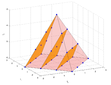
Figure 1: The states of iur’s of $su(2,1)$ represented by points in the three dark planes corresponding to $\Phi^{0}_{\ell}$ with $\ell=(0,0,-3)$, $\ell=(1,0,-4)$ and $\ell=(2,0,-5)$. All of them share the same energy.

Since the expression (4.6) for $E^{0}_{\ell}$ depends on $l_{0}+l_{2}$, it means that states in the family of iur’s derived from fundamental states (4.5) such that have the same value of $l_{0}+l_{2}$ will also have the same energy eigenvalue. It is worth to remark that the energy in (4.6) corresponding to bound states is negative, which is consistent with the expressions (2.5) and (2.8) for the Hamiltonians, and that the set of such bound states for each Hamiltonian is finite.

In Fig. 1, by means of an example, we represent the states of some iur’s by points $(l_{0},l_{1},l_{2})\in\mathbb{R}^{3}$ linked to the ground state $\Phi^{0}_{\ell}$, represented by the point $(l_{0},0,l_{2})$, through the raising operators $\hat{A}^{+},\hat{C}^{+}$. The points belonging to a iur are in a 2-dimensional plane (corresponding to the particular value of ${\cal C}^{\prime}$), and other iur’s are described by points in parallel 2D planes. These parallel planes are closed inside a tetrahedral unbounded pyramid whose basis extends towards $l_{2}\to-\infty$.

As in the case of $su(3)$ representations[15], in the above $su(2,1)$ iur’s we have some points (in the parameter space) which are degenerated, that is, they correspond to an eigen-space whose dimension is greater than one. For example, let us consider first the representation based on the fundamental state $\Phi^{0}_{\ell}$ with values $\ell=(0,0,-3)$. From this state we can build a iur made of points in a triangle, where each point represents a non-degenerate 1-dimensional (1D) eigenspace. Now, consider the iur corresponding to the ground state with $\ell_{0}=(1,0,-4)$, which has eigenstates with the same energy $E=-(-3+3/2)(-3+5/2)$ as the previous one (they have the same value of $l_{0}+l_{2}=-3$). Now the eigenstates corresponding to $\ell_{1}=(0,0,-5)$, inside this representation, can be obtained in two ways:

$$\Phi_{\ell_{1}}=\hat{C}^{+}\hat{A}^{+}\Phi_{\ell_{0}},\quad\tilde{\Phi}_{\ell_{1}}=\hat{A}^{+}\hat{C}^{+}\Phi_{\ell_{0}}\,.$$ (4.7)

It can be shown that these states are independent and that they span the 2D eigenspace of the corresponding Hamiltonian $H_{\ell_{1}}$ for that eigenvalue.

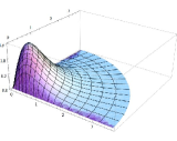
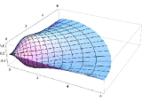
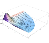
Figure 2: Plot of the orthogonal normalized eigenfunctions $\Phi(\theta,\xi)$, $0<\theta<\pi/2$, $0<\xi<\infty$, of $H_{\ell}$, for $\ell=(0,0,-5)$ corresponding to the ground state (left) and two independent states generating the eigenspace of the second (and last) excited energy level.

Remark that the ground state for the Hamiltonian $H_{\ell_{1}}$, $\ell_{1}=(0,0,-5)$, is given by the wavefunction (4.5) and its ground energy is $E^{0}_{\ell_{1}}=-(-5+3/2)(-5+5/2)$. The plot of the ground wavefunction and two independent excited wavefunctions are shown in Fig. 2.

Following the same pattern it can be obtained the degeneration of higher excited levels in the discrete spectrum: the $n$ excited level, when it exists, has associated an eigenspace with dimension $n$.

5 The complete symmetry algebra ${so(4,2)}$

As it is explicit from its expression (2.1) the Hamiltonian $H_{\ell}$ is invariant under reflections

$$\begin{array}[]{l}I_{0}:(l_{0},l_{1},l_{2})\to(-l_{0},l_{1},l_{2})\\[6.45831pt] I_{1}:(l_{0},l_{1},l_{2})\to(l_{0},-l_{1},l_{2})\\[6.45831pt] I_{2}:(l_{0},l_{1},l_{2})\to(l_{0},l_{1},-l_{2})\,.\end{array}$$ (5.1)

These operators can generate, by means of conjugation, other sets of intertwining operators from the ones already defined. For instance,

$$I_{0}:\{\hat{A}^{\pm},\hat{A}\}\to\{\tilde{A}^{\pm}=I_{0}\hat{A}^{\pm}I_{0},\tilde{A}=I_{0}\hat{A}I_{0}\}$$ (5.2)

where, from (3.1) we get

$$\tilde{A}_{l_{0},l_{1}}^{\pm}=\pm\partial_{\theta}-(-l_{0}+1/2)\,{\tan{\theta}}+(l_{1}+1/2)\,{\cot{\theta}},\quad\tilde{\lambda}_{l_{0},l_{1}}=(1-l_{0}+l_{1})^{2}$$ (5.3)

such that

$$\tilde{A}_{l_{0},l_{1}}^{-}:f_{l_{0},l_{1}}\rightarrow f_{l_{0}-1,l_{1}+1},\quad\tilde{A}_{l_{0},l_{1}}^{+}:f_{l_{0-1},l_{1}+1}\rightarrow f_{l_{0},l_{1}}\,.$$

Thus, we can define the operators $\tilde{A}^{\pm}$ as in (3.4) that together with $\tilde{A}\,f_{l_{0},l_{1}}:=-\frac{1}{2}\,(-l_{0}+l_{1})\,f_{l_{0},l_{1}}$ close a second $\widetilde{su}(2)$.

Other sets of operators $\{\tilde{B}^{\pm},\tilde{B}\}$ and $\{\tilde{C}^{\pm},\tilde{C}\}$, closing $\widetilde{su}(1,1)$ Lie algebras, can also be defined with the help of these reflections in the following way (the choice is non unique)

$$\begin{array}[]{l}I_{0}:\{\hat{A}^{\pm},\hat{A};\ \hat{B}^{\pm},\hat{B};\ \hat{C}^{\pm},\hat{C}\}\to\{\tilde{A}^{\pm},\tilde{A};\ \tilde{B}^{\pm},\tilde{B};\ C^{\pm},C\}\\[6.45831pt] I_{1}:\{\hat{A}^{\pm},\hat{A};\ \hat{B}^{\pm},\hat{B};\ \hat{C}^{\pm},\hat{C}\}\to\{\tilde{A}^{\mp},-\tilde{A};\ B^{\pm},B;\ \tilde{C}^{\pm},\tilde{C}\}\\[6.45831pt] I_{2}:\{\hat{A}^{\pm},\hat{A};\ \hat{B}^{\pm},\hat{B};\ \hat{C}^{\pm},\hat{C}\}\to\{A^{\pm},A;\ \tilde{B}^{\mp},-\tilde{B};\ -\tilde{C}^{\mp},-\tilde{C}\}\,.\end{array}$$ (5.4)

The whole set of the operators

$$\{\hat{A}^{\pm},\tilde{A}^{\pm},\hat{B}^{\pm},\tilde{B}^{\pm},\hat{C}^{\pm},\tilde{C}^{\pm},L_{0},L_{1},L_{2}\}$$ (5.5)

where the diagonal operators $L_{i}$ are defined as

$$L_{i}\Psi_{\ell}=l_{i}\Psi_{\ell}$$ (5.6)

generate an $o(4,2)$ Lie algebra of rank three with commutations rules that can be easily derived from those of $su(2,1)$ given in (4) and the action of the reflections (5.4). These generators link eigenstates of the Hamiltonians $H_{\ell}$ with the same eigenvalue.

Now, consider a fundamental state $\Psi^{0}_{\ell}$ for the $so(4,2)$ algebra annihilated by the lowering operators,

$$A^{-}_{\ell}\Psi^{0}_{\ell}=\tilde{A}^{-}_{\ell}\Psi^{0}_{\ell}=C^{-}_{\ell}\Psi^{0}_{\ell}=\tilde{C}^{-}_{\ell}\Psi^{0}_{\ell}=B^{-}_{\ell}\Psi^{0}_{\ell}=\tilde{B}^{-}_{\ell}\Psi^{0}_{\ell}=0\,.$$ (5.7)

This state should be a particular case of (4.5) invariant also under the $l_{0}$-reflection:

$$\Phi^{0}_{\ell}(\xi,\theta)=N(\cos\theta)^{1/2}(\sin\theta)^{1/2}(\cosh\xi)^{l_{2}+1/2}\sinh\xi,$$ (5.8)

thus, it has the label $\ell=(l_{0}=0,l_{1}=0,l_{2})$, where $l_{2}<-5/2$. This point in the parameter space, for the example of Fig. 1, corresponds to the top vertex of the pyramid, from which all the other points displayed in the figure can be obtained with the help of raising operators. Such points correspond to a iur of the $so(4,2)$ algebra, including the series of iur’s of the $su(2,1)$ algebra mentioned in the previous section.

Fixed the iur corresponding to $\ell=(0,0,l_{2})$ such that $-7/2\leq l_{2}<-5/2$, then, the points on the surface of the associated pyramid in the parameter space correspond to non-degenerated ground levels of their respective Hamiltonians. This ‘top’ pyramid includes other ‘inner’ pyramids, see Fig. 3, with vertexes $\ell_{n}=(0,0,l_{2}-2n)$. Each point on the surface of an inner pyramid associated to $\ell_{n}$ represents an $n$-excited level $(n+1)$-fold degenerated of the iur associated to $\ell$.

Finally, we must remark that the same set of Hamiltonians and eigenstates can be described by ‘dual’ representations of $so(4,2)$ (or $su(2,1)$) by means of inverted pyramids with positive values of $l_{2}$ fixing the inverted vertex.

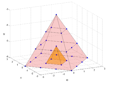
Figure 3: It is shown two pyramids associated to the same iur of $so(4,2)$. The exterior with vertex $(0,0,-3)$ has points on its exterior faces which represent non-degenerated levels. The inner one has exterior faces corresponding to first excited double-degenerated levels.

6 Concluding remarks

In this work we have built a set of intertwining operators for a superintegrable system defined on a two-sheet hyperboloid and we have found that they close a non-compact $su(2,1)$ Lie algebra structure. By using the reflections operators of the system we have implemented these IO’s obtaining an $so(4,2)$ algebra. These IO’s lead to hierarchies of Hamiltonians described by points on planes ($su(2,1)$) or in the 3D space ($so(4,2)$), corresponding to the rank of the respective Lie algebra.

We have shown how these IO’s can be very helpful in the characterization of the physical system by selecting separable coordinates, determining the eigenvalues and building eigenfunctions. We have also displayed the relation of eigenstates and eigenvalues with unitary representations of the $su(2,1)$ and $so(4,2)$ Lie algebras. In particular we have studied the degeneration problem as well as the number of bound states. Remark that such a detailed study of a ‘non-compact’ superintegrable system has not been realized till now, up to our knowledge.

We have restricted to iur’s, but a wider analysis can be done for hierarchies associated to representations with a not well defined unitary character.

The IO’s can also be used to find the second order integrals of motion for a Hamiltonian $H_{\ell}$ and their algebraic relations, which is the usual approach to (super) integrable systems. However, we see that it is much easier to deal directly with the IO’s, which are more elementary and simpler, than with constants of motion.

Our program in the near future is the application of this method to wider situations. Besides, in principle, we can also adapt the method to classical versions of such systems. On this aspect we must remark that some symmetry procedures usually considered only for quantum systems can be extended in an appropriate way to classical ones [18].

References

References

• [1] del Olmo M A, Rodríguez M A and Winternitz P 1993 J. Math. Phys. 34 5118
• [2] Kalnins E G, Miller W and Pogosyan G S 1996 J. Math. Phys. 37 6439
• [3] del Olmo M A, Rodríguez M A and Winternitz P 1996 Fortschritte der Physik, 44, 91
• [4] Calzada J A, del Olmo M A and Rodríguez M A 1997 J. Geom. Phys. 23 14
• [5] Calzada J A, del Olmo M A and Rodriguez M A 1999 J. Math. Phys. 40 88
• [6] Calzada J A, Negro J, del Olmo M A and Rodríguez M A 1999 J. Math. Phys. 41 317
• [7] Rañada M F 2000 J. Math. Phys. 41 2121
• [8] Rañada M F and Santander M 2003 J. Math. Phys. 44 2149
• [9] Evans N W 1990 Phys. Rev. 41 5666 1990 Phys. Lett. 147A 483 1991 J. Math. Phys. 32 3369
• [10] Matveev V B and Salle M A 1991 Darboux Transformations and Solitons (Berlin: Springer)
• [11] Kuru Ş, Teǧmen A and Verçin A 2001 J. Math. Phys. 42 3344
• [12] Demircioǧlu B, Kuru Ş, Önder M and Verçin A 2002 J. Math. Phys. 43 2133
• [13] Samani K A and Zarei M 2005 Ann. Phys. 316 466
• [14] Fernández D J, Negro J and del Olmo M A 1996 Ann. Phys. 252 386
• [15] Calzada J A, Negro J and del Olmo M A 2006 J. Math. Phys. 47 043511
• [16] Barut A O, Inomata A and Wilson R 1987 J. Phys. A 20 4075 1987 J. Phys. A 20 4083
• [17] del Sol Mesa A, Quesne C and Smirnov Yu F 1998 J. Phys. A 31 321
• [18] Kuru Ş and Negro J 2008 Ann. Phys. 323 413